Appendix B
Programming Machine Learning in Python
B.1 PRE-REQUISITES
B.1.1 Install anaconda in your system
Before starting to do machine learning programming in Python, please install Python Anaconda distribution from https://anaconda.org/anaconda/python. To write any python script, open any text editor and write your python script and save with the extension .py. You may also use the Spyder (Scientific PYthon Development EnviRonment), which is a powerful and interactive development environment for the Python language with advanced editing, interactive testing, debugging, and introspection features. In this chapter, all the examples have been created working in Spyder.
B.1.2 Know how to manage Python scripts
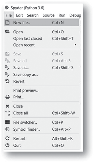
- Open new/pre-existing .py script in Spyder as shown in Figure B.1:
B.1.3 Know how to do basic programming using Python
B.1.3.1 Introduction to basic Python commands
First install a couple of basic libraries of Python namely
- ‘os’ for using operating system dependent functions
- ‘pandas’ for extensive data manipulation functionalities
In general, Annaconda Python by default contains all the basic required packages for starting programming in machine learning. But in case, any extra package is needed, ‘pip’ is the recommended installer.
Command: pip install
Syntax: pip install ‘SomePackage’
After installing, libraries need to be loaded by invoking the command:
Command: import <<library-name>>
Syntax: import os
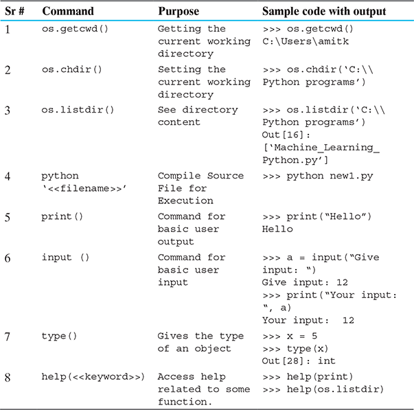
Try out each of the following commands.
B.1.3.2 Basic data types in Python
Python has five standard data types −
- Number
- String
- List
- Tuple
- Dictionary
Though Python has all the basic data types, Python variables do not need explicit declaration to reserve memory space. The declaration happens automatically when you assign a value to a variable. The equal sign (=) is used to assign values to variables.
The operand to the left of the = operator is the name of the variable and the operand to the right of the = operator is the value stored in the variable. For example −
>>> var1 = 4
>>> var2 = 8.83
>>> var3 = “Machine Learning”
>>> type(var1)
Out[38]: int
>>> print(var1)
4
>>> type(var2)
Out[39]: float
>>> print(var2)
8.83
>>> type(var3)
Out[40]: str
>>> print(var3)
Machine Learning
Python variables can be easily typecasted from one data type to another by using its datatype name as a function (actually a wrapper class) and passing the variable to be typecasted as a parameter. But not all data types can be transformed into another like String to integer/number is impossible (that’s obvious!).
>>> var2 = int(var2)
>>> print (var2)
8
>>> type (var2)
Out[42]: int
B.1.3.3 for–while Loops & if–else Statement
For loop
Syntax:
for i in range(<lowerbound>,<upperbound>,<interval>):
print(i*i)
Example: Printing squares of all integers from 1 to 3.
for i in range(1,4):
print(i*i)
1
4
9
for i in range(0,4,2):
print(i)
2
4
While loop
Syntax:
while < condition>:
<do something>
Example: Printing squares of all integers from 1 to 3.
i = 0
while i < 5:
print(i*i)
i = i + 1
1
4
9
if-else statement
Syntax:
if < condition>:
<do something>
else:
<do something else>
Example: Printing squares of all integers from 1 to 3.
i = -5
if i < 0:
print(i*i)
else:
print(i)
25
B.1.3.4 Writing functions
Writing a function (in a script):
Syntax:
def functionname(parametername,…):
(function_body)
Example: Function to calculate factorial of an input number n.
def factorial(n):
fact = 1
for i in range(1,n+1):
fact = fact*i
return(fact);
Running the function (after compiling the script using source (“script_name”):
>>> factorial(6)
720
B.1.3.5 Mathematical operations on data types
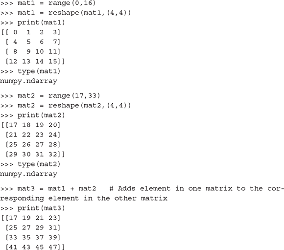
Vectors:
>>> n = 10
>>> m = 5
>>> n + m #addition
Out[53]: 15
>>> n - m #subtraction
Out[55]: 5
>>> n * m #multiplication
Out[56]: 50
>>> n / m #division
Out[57]: 2.0
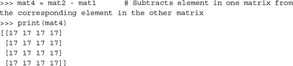
Matrices:
Note:
pandas is a Python package providing fast and flexible functionalities designed to work with “relational” or “labelled” data.
B.1.3.6 Basic data handling commands
>>> import pandas as pd # “pd” is just an alias for pandas
>>> data = pd.read_csv(“auto-mpg.csv”) # Uploads data from a .csv file
>>> type(data) # To find the type of the data set object loaded pandas.core.frame.DataFrame
>>> data.shape # To find the dimensions i.e. number of rows and columns of the data set loaded
(398, 9)
>>> nrow_count = data.shape[0] # To find just the number of rows
>>> print(nrow_count)
398
>>> ncol_count = data.shape[1] # To find just the number of columns
>>> print(ncol_count)
9
>>> data.columns # To get the columns of a dataframe
Index([‘mpg’, ‘cylinders’, ‘displacement’, ‘horsepower’, ‘weight’, ‘acceleration’, ‘model year’, ‘origin’, ‘car name’],
dtype=’object’)
>>> list(data.columns.values)# To list the column names of a dataframe
We can also use:
>>> list(data)
[‘mpg’,
‘cylinders’,
‘displacement’,
‘horsepower’,
‘acceleration’,
‘model year’,
‘origin’,
‘car name’]
# To change the columns of a dataframe …
>>> data.columns = [‘miles_per_gallon’, ‘cylinders’, ‘displacement’, ‘horsepower’, ‘weight’, ‘acceleration’, ‘model year’, ‘origin’, ‘car name’]
Alternatively, we can use the following code:
>>> data.rename(columns={‘displacement’: ‘disp’}, inplace=True)
>>> data.head() # By default displays top 5 rows
>>> data.head(3) # To display the top 3 rows
>>> data. tail () # By default displays bottom 5 rows
>>> data. tail (3) # To display the bottom 3 rows
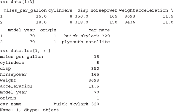
>>> data.at[200,’cylinders’] # Will return cell value of the 200th row and column ‘cylinders’ of the data frame
6
Alternatively, we can use the following code:
>>> data.get_value(200,’cylinders’)
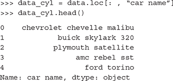
To select a specific column of a dataframe:
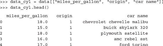
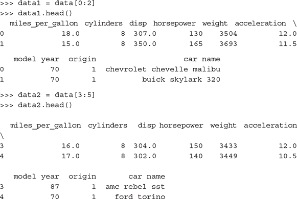
To select multiple columns of a dataframe:
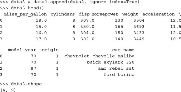
Bind sets of rows of dataframes:
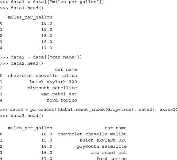
Bind sets of columns of dataframes:
To save dataframes as .csv files:
>>> data3.to_csv(‘data3.csv’) #Save dataframe with index column
>>> data3.to_csv(‘data3.csv’, index=False) #Save dataframe without index column
Often, we get data sets with duplicate rows, which is nothing but noise. Therefore, before training the model, we need to make sure we get rid of such inconsistencies in the data set. We can remove duplicate rows using code:
>>> data = data.drop_duplicates()
We frequently find missing values in our data set. We can drop the rows/columns with missing values using the code below.
>>> data.dropna(axis=0, how=’all’) #Remove all rows where values of all columns are ‘NaN’
>>> data.dropna(axis=1, how=’all’) ) #Remove all columns where values of all rows are ‘NaN’
>>> data.dropna(axis=0, how=’any’) #Remove all rows where value of any column is ‘NaN’
>>> data.dropna(axis=1, how=’any’) ) #Remove all columns where value of any row is ‘NaN’
B.2 PREPARING TO MODEL
Now that we are kind of familiar with the basic Python commands, we have the ability to start machine learning programming in Python. But before starting to do actual modelling work, we have to first understand the data using the concepts highlighted in Chapter 2. Also, there might be some issues in the data which you will unveil during data exploration. You have to remediate that too.
So first, let’s find out how to do data exploration in Python. There are two ways to explore and understand data:
- By using certain statistical functions to understand the central tendency and spread of the data
- By visually observing the data in the form of plots or graphs
B.2.1 Basic statistical functions for data exploration
Let’s start with the first approach of understanding the data through the statistical techniques. As we have seen in Chapter 2, for any data set, it is critical to understand the central tendency and spread of the data. We have also seen the standard statistical measures are as follows:
- Measures of central tendency – Mean, median, mode
- Measures of data spread
- Dispersion of data – variance, standard deviation
- Position of the different data values – quartiles, inter-quartile range (IQR)
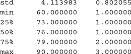
In Python, info function provides the structure of the data frame along with the data types of the different attributes. Also, there is a function describe which generates the summary statistics of a data set. It gives the first basic understanding of the data set which can trigger thought about the data set and the anomalies that may be present. So, let’s start off exploring a data set Auto MPG data set from the University of California, Irvine (UCI) machine learning repository. We will run the info and describe commands for the Auto MPG data set.
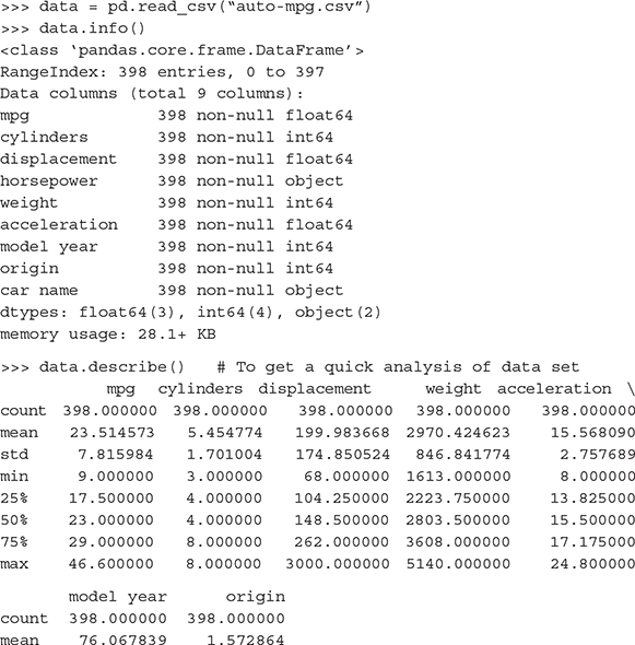
Looking closely at the output of the describe command, there are seven measures listed for the attributes (well, most of them). These are
- mean – mean of the specific attribute
- std – Standard deviation of the specific attribute
- min – minimum value of the attribute
- 25% – First quartile (for details, refer to Chapter 2)
- 50% – Median of the attribute
- 75% – Third quartile (for details, refer to Chapter 2)
- max – maximum value of the attribute
These gives a pretty good understanding of the data set attributes. Now, note that one attribute – car.name, has a data type object whereas the remaining attributes have either integer or float data type. Why is that so? This is because this attribute is a categorical attribute while the other ones are numeric.
Note:
Numpy is a Python library which is used for scientific computing. It contains among other things – a powerful array object, mathematical and statistical functions, and tools for integrating with C/C++ and Fortran code.
Let’s try to explore if any variable has any problem with the data values where a cleaning may be required. As discussed in Chapter 2, there may be two primary data issues – missing values and outliers.
Let’s first try to figure out if there is any missing value for any of the attributes. Let’s use a small piece of Python code find out if there is any missing/unwanted value for an attribute in the data. If there is, return the rows in which the attribute has missing/unwanted values. Checking for all the attributes, we find that the attribute ‘horsepower’ has missing values.
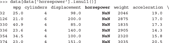
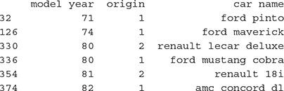
There are six rows in the data set which have missing values for the attribute ‘horsepower’. We will have to remediate these rows before we proceed with the modelling activities. We will do that shortly.
The easiest and most effective way to detect outliers is from the box plot of the attributes. In the box plot, outliers are very clearly highlighted. When we explore the attributes using box plots in a short while, we will have a clear view of this.
We can get the other statistical measure of the attributes using the following Python commands from the Numpy library:
>>> np.mean(data[[“mpg”]])
23.514573
>>> np.median(data[[“mpg”]])
23.0
>>> np.var(data[[“mpg”]])
60.936119
>>> np.std(data[[“mpg”]])
7.806159
Note:
Matplotlib is a plotting library for the Python programming language which produces 2D plots to render visualization and helps in exploring the data sets. mat-plotlib.pyplot is a collection of command style functions that make matplotlib work like MATLAB
B.2.2 Basic plots for data exploration
In order to start using the library functions of matplotlib, we need to include the library as follows:
>>> import matplotlib.pyplot as plt
Let’s now understand the different graphs that are used for data exploration and how to generate them using Python code.
We will use the “iris” data set, a very popular data set in the machine learning world. This data set consists of three different types of iris flower: Setosa, Versicolour, and Virginica, the columns of the data set being - Sepal Length, Sepal Width, Petal Length, and Petal Width. For using this data set, we will first have to import the Python library datasets using the code below.
>>> from sklearn import datasets
# import some data to play with
>>> iris = datasets.load_iris()
B.2.2.1 Box plot
>>> import matplotlib.pyplot as plt
>>> X = iris.data[:, :4]
>>> plt.boxplot(X)
>>> plt.show()
A box plot for each of the four predictors is generated as shown in Figure B.2.
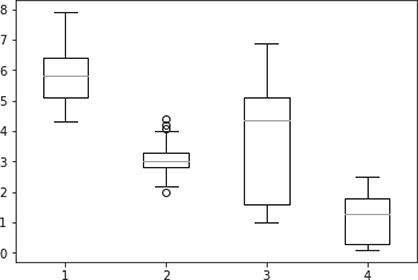
FIG. B.2 Box plot for an entire data set
As we can see, Figure B.2 gives the box plot for the entire iris data set i.e. for all the features in the iris data set, there is a component or box plot in the overall plot. However, if we want to review individual features separately, we can do that too using the following Python command.
>>> plt.boxplot(X[:, 1])
>>> plt.show()
The output of the command i.e. the box plot of an individual feature, sepal width, of the iris data set is shown in Figure B.3.
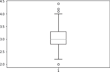
FIG. B.3 Box plot for a specific feature
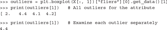
To find out the outliers of an attribute, we can use the code below:
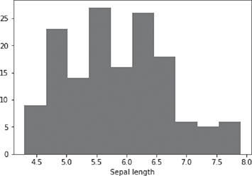
B.2.2.2 Histogram
>>> import matplotlib.pyplot as plt
>>> X = iris.data[:, :1]
>>> plt.hist(X)
>>> plt.xlabel(‘Sepal length’)
>>> plt.show()
The output of the command, i.e. the histogram of an individual feature, Sepal Length, of the iris data set is shown in Figure B.4.
B.2.2.3 Scatterplot
>>> X = iris.data[:, :4] # We take the first 4 features
>>> y = iris.target
>>> plt.scatter(X[:, 2], X[:, 0], c=y, cmap=plt.cm.Set1, edgecolor=’k’)
>>> plt.xlabel(‘Petal length’)
>>> plt.ylabel(‘Sepal length’)
>>> plt.show()
The output of the command, i.e. the scatter plot for the feature pair petal length and sepal length of the iris data set is shown in Figure B.5.
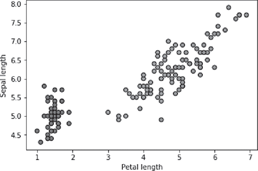
FIG. B.5 Scatter plot of Petal Length vs. Sepal Length
B.2.3 Data pre-processing
The primary data pre-processing activities are remediating data issues related to outliers and missing values. Also, feature subset selection is quite a critical area of data pre-processing. Let’s understand how to write programs for achieving these purposes.
B.2.3.1 Handling outliers and missing values
As we saw in Chapter 2, the primary measures for remediating outliers and missing values are
- Removing specific rows containing outliers/missing values
- Imputing the value (i.e. outliers/missing value) with a standard statistical measure, e.g. mean or median or mode for that attribute
- Estimate the value (i.e. outlier / missing value) based on value of the attribute in similar records and replace with the estimated value.
- Cap the values within 1.5 X IQR limits
B.2.3.1.1 Removing outliers / missing values
We have to first identify the outliers. We have already seen in boxplots that outliers are clearly found out when we draw the box plot of a specific attribute. Hence, we can use the same concept as shown in the following code:
>>> outliers = plt.boxplot(X[:, 1])[“fliers”][0].get_data()[1]
There is an alternate option too. As we know, outliers have abnormally high or low value from other elements. So the other option is to use threshold values to detect outliers so that they can be removed. A sample code is given below.
def find_outlier(ds, col):
quart1 = ds[col].quantile(0.25)
quart3 = ds[col].quantile(0.75)
IQR = quart3 - quart1 #Inter-quartile range
low_val = quart1 - 1.5*IQR
high_val = quart3 + 1.5*IQR
ds = ds.loc[(ds[col] < low_val) | (ds[col] > high_val)]
return ds
>>> outliers = find_outlier(data, “mpg”)
Then those rows can be removed using the code:
def remove_outlier(ds, col):
quart1 = ds[col].quantile(0.25)
quart3 = ds[col].quantile(0.75)
IQR = quart3 - quart1 #Interquartile range
low_val = quart1 - 1.5*IQR
high_val = quart3 + 1.5*IQR
df_out = ds.loc[(ds[col] > low_val) & (ds[col] < high_val)]
return df_out
>>> data = remove_outlier(data, “mpg”)
Rows having missing values can be removed using the code:
>>> data.dropna(axis=0, how=’any’) #Remove all rows where value of any column is ‘NaN’
B.2.3.1.2 Imputing standard values
The code for identification of outliers or missing values will remain the same. For imputation, depending on which statistical function is to be used for imputation, code will be as follows:
Only the affected rows are identified and the value of the attribute is transformed to the mean value of the attribute.
>>> hp_mean = np.mean(data[‘horsepower’])
>>> imputedrows = data[data[‘horsepower’].isnull()]
>>> imputedrows = imputedrows.replace(np.nan, hp_mean)
Then the portion of the data set not having any missing row is kept apart.
>>> missval_removed_rows = data.dropna(subset=[‘horsepower’])
Then join back the imputed rows and the remaining part of the data set.
>>> data_mod = missval_removed_rows.append(imputedrows, ignore_index=True)
In a similar way, outlier values can be imputed. Only difference will be in identification of the relevant rows.
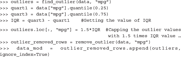
B.2.3.1.3 Capping of values
The code for identification of outliers values will remain the same. For capping, generally a value 1.5 times the (inter-quartile range) IQR is to be used for imputation, code will be as follows:
Note:
Scikit-learn (“SciKit” = SciPy Toolkit) is a machine learning library for the Python programming language. It contains various classification, regression and clustering algorithms including support vector machines, random forests, gradient boosting, k-means, etc. Built on NumPy, SciPy, and matplotlib, it is designed to interoperate smoothly between the libraries.
B.3 MODEL TRAINING
B.3.1 Holdout
The first step before starting to model, in case of supervised learning, is to load the input data, hold out a portion of the input data as test data and have the remaining portion as training data for building the model. Below is the standard way to do it. Scikit-learn provides a function to split input data set into training and test data sets.
>>> import pandas as pd
>>> data = pd.read_csv(“btissue.csv”)
>>> from sklearn.model_selection import train_test_split
>>> data.shape
(106, 10)
>>> data_train, data_test = train_test_split(data, test_size = 0.3, random_state = 123) # The parameter test_size sets the ratio of test data to the input data to 0.3 or 30% and random_state sets the seed for random number generator
>>> len(data_train)
74
>>> len(data_test)
32
Note:
When we do data holdout, i.e. splitting of the input data into training and test data sets, the records selected for each set are picked randomly. So, it is obvious that executing the same code may result in different training data set. So the model trained will also be somewhat different. In Python Scikit function train_test_split, the parameter random_state sets the starting point of the random number generator used internally to pick the records. This ensures that random numbers of a specific sequence is used every time and hence the same records (i.e. records having same sequence number) are picked every time and the model is trained in the same way. This is extremely critical for the reproducibility of results i.e. every time, the same machine learning program generates the same set of results.
B.3.2 K-fold cross-validation
Let’s do k-fold cross-validation with 10 folds. For creating the cross-validation, there are two options. KFold function of either sklearn.cross_validation or sklearn.model_ selection can be used as follows:
>>> import pandas as pd
>>> data = pd.read_csv(“auto-mpg.csv”)
>>> from sklearn.cross_validation import KFold
>>> kf = KFold(data.shape[0], n_folds=10, random_state=123)
>>> for train_index, test_index in kf:
data_train = data.iloc[train_index]
data_test = data.iloc[test_index]
# Option 2
>>> from sklearn.model_selection import KFold
>>> kf = KFold(n_splits=10)
>>> for train, test in kf.split(data):
data_train = data.iloc[train_index]
data_test = data.iloc[test_index]
B.3.3 Bootstrap sampling
As discussed in Capter 3, bootstrap resampling is used to generate samples of any given size from the training data. It uses the concept of simple random sampling with repetition. To generate bootstrap sample in Python, resample function of sklearn.utils library can be used. Below is a sample code
>>> import pandas as pd
>>> from sklearn.utils import resample
>>> data = pd.read_csv(“btissue.csv”)
>>> X = data.iloc[:,0:9]
>>> X
>>> resample(X, n_samples=200, random_state=0) # Generates a sample of size 200 (as mentioned in parameter n_samples) with repetition …
B.3.4 Training the model
Once the model preparatory steps, like data holdout, etc. are over, the actual training happens. The sklearn framework in Python provides most of the models which are generally used in machine learning. Below is a sample code.
>>> from sklearn.tree import DecisionTreeClassifier
>>> predictors = data.iloc[:,0:7] # Segregating the predictors
>>> target = data.iloc[:,7] # Segregating the target/class
>>> predictors_train, predictors_test, target_train, target_test = train_test_split(predictors, target, test_size = 0.3, random_state = 123) # Holdout of data
>>> dtree_entropy = DecisionTreeClassifier(criterion = “entropy”, random_state = 100, max_depth=3, min_samples_leaf=5) #Model is initialized
# Finally the model is trained
>>> model = dtree_entropy.fit(predictors_train, target_train)
B.3.5 Evaluating model performance
B.3.5.1 Supervised learning - classification
As we have already seen in Chapter 3, the primary measure of performance of a classification model is its accuracy. Accuracy of a model is calculated based on correct classifications made by the model compared to total number of classifications. In Python, sklearn.metrics provides accuracy_score functionality to evaluate the accuracy of a classification model. Below is the code for evaluating the accuracy of a classifier model.
>>> prediction = rf.predict(predictors_test)
>>> accuracy_score(target_test, prediction, normalize = True)
The confusion_matrix functionality of sklearn.metrics helps in generation the confusion matrix, discussed in detail in Chapter 3. Below is the code for finding the confusion matrix of a classifier model. Also, in Figure B.6, is a quick analysis of the output confusion matrix as obtained from the Python code.
>>> confusion_matrix(target_test, prediction)
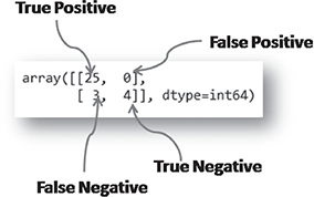
FIG. B.6 Performance evaluation of a classification model
B.3.5.2 Supervised learning - regression
We have seen in Chapter 3, R-squared is an effective measure of performance of a regression model. In Python, sklearn.metrics provides mean_squared_error and r2_score functionality to evaluate the accuracy of a regression model. Below is a sample code.
>>> prediction = model.predict(predictors_test)
>>> mean_squared_error(target_test, prediction)
>>> r2_score(target_test, prediction)
B.3.5.3 Unsupervised learning - clustering
As we have seen in Chapter 3, there are two popular measures of cluster quality – purity and silhouette width. Purity can be calculated only when class label is known for the data set subjected to clustering. On the other hand, silhouette width can be calculated for any data set.
Purity
We will use a Lower Back Pain Symptoms data set released by Kaggle (https://www.kaggle.com/sammy123/lower-back-pain-symptoms-dataset). The data set consists of 310 observations, 13 attributes (12 numeric predictors, 1 binary class attribute).
>>> import pandas as pd
>>> import numpy as np
>>> from sklearn.cluster import KMeans
>>> from sklearn.metrics.cluster import v_measure_score
>>> data = pd.read_csv(“spine.csv”)
>>> data_woc = data.iloc[:,0:12] # Stripping out the class variable from the data set …
>>> data_class = data.iloc[:,12] # Segregating the target / class variable …
>>> f1 = data_woc[‘pelvic_incidence’].values
>>> f2 = data_woc[‘pelvic_radius’].values
>>> f3 = data_woc[‘thoracic_slope’].values
>>> X = np.array(list(zip(f1, f2, f3)))
>>> kmeans = KMeans(n_clusters = 2, random_state = 123)
>>> model = kmeans.fit(X)
>>> cluster_labels = kmeans.predict(X)
>>> v_measure_score(cluster_labels, data_class)
Output
0.12267025741680369
Silhouette Width
For calculating Silhouette Width, silhouette_score function of sklearn. metrics library can be used for calculating Silhouette width. Below is the code for calculating Silhouette Width. A full implementation can be found in a later section A.5.3.
>>> from sklearn.metrics import silhouette_score
>>> sil = silhouette_score(X, cluster_labels, metric = ’euclidean’,sample_size = len(data)) # “X” is a feature matrix for the feature subset selected for clustering and “data” is the data set
B.4 FEATURE ENGINEERING
B.4.1 Feature construction
For doing feature construction, we can use pandas library of Python. Following is a small code for implementing feature construction.
>>> import pandas as pd
>>> room_length = [18, 20, 10, 12, 18, 11]
>>> room_breadth = [20, 20, 10, 11, 19, 10]
>>> room_type = [‘Big’, ‘Big’, ‘Normal’, ‘Normal’, ‘Big’, ‘Normal’]
>>> data = pd.DataFrame({‘Length’: room_length, ‘Breadth’: room_ breadth, ‘Type’: room_type})
>>> data
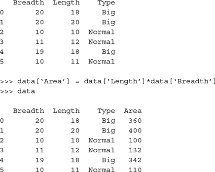
B.4.1.1 Dummy coding categorical (nominal) variables:
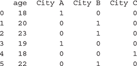
get_dummies function of pandas library can be used to dummy code categorical variables. Following is a sample code for the same.
>>> import pandas as pd
>>> age = [18, 20, 23, 19, 18, 22]
>>> city = [‘City A’, ‘City B’, ‘City B’, ‘City A’, ‘City C’, ‘City B’]
>>> data = pd.DataFrame({‘age’: age, ‘city’: city})
>>> data
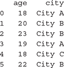
>>> dummy_features = pd.get_dummies(data[‘city’])
>>> data_age = pd.DataFrame(data = data, columns = [‘age’])
>>> data_mod = pd.concat([data_age.reset_index(drop=True), dummy_ features], axis=1)
>>> data_mod
B.4.1.2 Encoding categorical (ordinal) variables:
LabelEncoder function of sklearn. preprocessing library can be used to encode categorical variables. Following is a sample code for the same.
>>> import pandas as pd
>>> from sklearn import preprocessing
>>> marks_science = [78,56,87,91,45,62]
>>> marks_maths = [75,62,90,95,42,57]
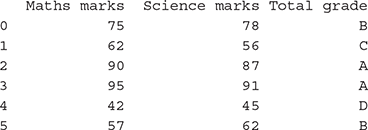
>>> grade = [‘B’,’C’,’A’,’A’,’D’,’B’]
>>> data = pd.DataFrame({‘Science marks’: marks_science, ‘Maths marks’: marks_maths, ‘Total grade’: grade})
>>> data
# Option 1
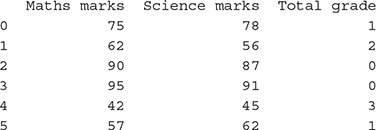
>>> le = preprocessing.LabelEncoder()
>>> le.fit(data[‘Total grade’])
>>> data[‘Total grade’] = le.transform(data[‘Total grade’])
>>> data
# Option 2
>>> target = data[‘Total grade’].replace([‘A’,’B’,’C’ ,’D’],[0,1,2,3])
>>> predictors = data.iloc[:, 0:2]
>>> data_mod = pd.concat([predictors.reset_index(drop=True), target], axis=1)
B.4.1.3 Transforming numeric (continuous) features to categorical features:
>>> import pandas as pd
>>> apartment_area = [4720, 2430, 4368, 3969, 6142, 7912]
>>> apartment_price = [2360000,1215000,2184000,1984500,3071000,3 956000]
>>> data = pd.DataFrame({‘Area’: apartment_area, ‘Price’: apartment_price})
>>> data

B.4.2 Feature extraction
B.4.2.1 Principal Component Analysis (PCA):
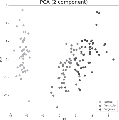
For doing principal component analysis or in other words – to get the principal components of a set of features in a data set, we can use PCA function of sklearn.decomposition library. However, features should be standardized (i.e. transform to unit scale with mean = 0 and variance = 1), for which StandardScaler function of sklearn. preprocessing library can be used. Following is the code using the iris data set. PCA should be applied on the predictors. The target / class variable can be used to visualize the principal components (Figure B.7).
>>> import pandas as pd
>>> import matplotlib.pyplot as plt
>>> from sklearn import datasets
>>> from sklearn.decomposition import PCA
>>> from sklearn.preprocessing import StandardScaler
>>> iris = datasets.load_iris()
>>> predictors = iris.data[:, 0:4]
>>> target = iris.target
>>> predictors = StandardScaler().fit_transform(predictors) # Standardizing the features
>>> pca = PCA(n_components=2)
>>> princomp = pca.fit_transform(predictors)
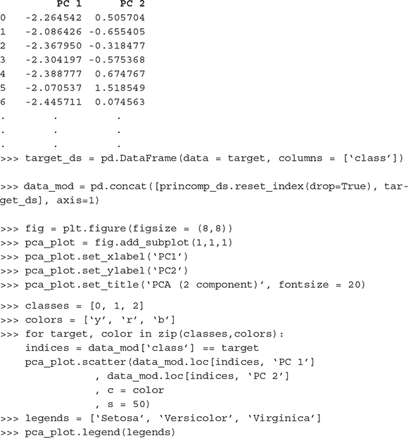
>>> princomp_ds = pd.DataFrame(data = princomp, columns = [‘PC 1’, ‘PC 2’])
>>> princomp_ds
B.4.2.2 Singular Value Decomposition (SVD):
We have seen in Chapter 4 that singular value decomposition of a matrix A (m X n) is a factorization of the form:
For implementing singular value decomposition in Python, we can use svd function of scipy.linalg library. Following is the code using the iris data set.
>>> import pandas as pd
>>> from sklearn import datasets
>>> from scipy.linalg import svd
>>> iris = datasets.load_iris()
>>> predictors = iris.data[:, 0:4]
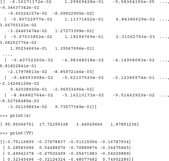
>>> U, s, VT = svd(predictors)
>>> print(U)
B.4.2.3 Linear Discriminant Analysis (LDA):
For implementing singular value decomposition in Python, we can use LinearDiscriminantAnalysis function of sklearn.discriminant_analysis library. Following is the code using the UCI data set btissue.
>>> import pandas as pd
>>> import numpy as np
>>> from sklearn import datasets
>>> from sklearn.discriminant_analysis import LinearDiscriminantAnalysis
>>> from sklearn.utils import column_or_1d
>>> data = pd.read_csv(“btissue.csv”)
>>> X = data.iloc[:,0:9]
>>> y = column_or_1d(data[‘class’], warn=True) #To generate 1d array, column_or_1d has been used …
>>> clf = LinearDiscriminantAnalysis()
>>> lda_fit = clf.fit(X, y)
>>> print(lda_fit)
LinearDiscriminantAnalysis(n_components=None, priors=None, shrinkage=None,solver=’svd’, store_covariance=False, tol=0.0001)
>>> pred = clf.predict([[1588.000000, 0.085908, -0.086323, 516.943603, 12895.342130, 25.933331, 141.722204, 416.175649, 1452.331924]])
>>> print(pred)
[‘con’]
B.4.3 Feature subset selection
Feature subset selection is a topic of intense research. There are many approaches to select a subset of features which can improve model performance. It is not possible to cover all such approaches as a part of this text. However, sklearn.feature_selection module can be used for applying basic feature selection. There are multiple options of feature selection offered by the module, one of which is presented below:
>>> import pandas as pd
>>> import numpy as np
>>> from sklearn.feature_selection import SelectKBest
>>> from sklearn.feature_selection import chi2
>>> data = pd.read_csv(“apndcts.csv”)
>>> predictors = data.iloc[:,0:7] # Seggretating the predictor variables …
>>> target = data.iloc[:,7] # Seggretating the target / class variable …
>>> test = SelectKBest(chi2, k=2)
>>> fit = test.fit(predictors, target)
>>> features = fit.transform(predictors)
>>> print(predictors.columns)
>>> np.set_printoptions(precision=3)
>>> print(fit.scores_)
Output:
Index([‘At1’, ‘ At2’, ‘ At3’, ‘ At4’, ‘ At5’, ‘ At6’, ‘ At7’], dtype=’object’)
Scores for each feature:
[ 1.771 1.627 2.391 1.084 1.673 1.647 2.236]
B.5 MACHINE LEARNING MODELS
B.5.1 Supervised learning - classification
In the chapter 6, 7, and 8, conceptual overview of different supervised learning algorithms has been presented. Now, you will get to know, how to implement them using Python. For the sake of simplicity, we have tried to keep the code for implementing each of the algorithms as consistent as possible. Also, we have used benchmark data sets from UCI repository (will also keep it available online).
B.5.1.1 Naive bayes classifier:
For Naive Bayes classifier implementation, GaussianNB library of sklearn.naive_ bayes has been used. The full code for the implementation is given below.
>>> import pandas as pd
>>> from sklearn.model_selection import train_test_split
>>> from sklearn.metrics import accuracy_score
>>> from sklearn.naive_bayes import GaussianNB
>>> data = pd.read_csv(“apndcts.csv”)
>>> predictors = data.iloc[:,0:7] # Segregating the predictor variables …
>>> target = data.iloc[:,7] # Segregating the target / class variable …
>>> predictors_train, predictors_test, target_train, target_test = train_test_split(predictors, target, test_size = 0.3, random_state = 123)
>>> gnb = GaussianNB()
# First train model / classifier with the input dataset (training data part of it)
>>> model = gnb.fit(predictors_train, target_train)
# Make prediction using the trained model
>>> prediction = model.predict(predictors_test)
# Time to check the prediction accuracy …
>>> accuracy_score(target_test, prediction, normalize = True)
Output Accuracy:
0.90625
B.5.1.2 kNN classifier:
k-Nearest Neighbour (kNN) classifier is implemented through KNeighborsClassifier library of sklearn. neighbors. The full code for the implementation is given below.
>>> import pandas as pd
>>> from sklearn.model_selection import train_test_split
>>> from sklearn.metrics import accuracy_score
>>> from sklearn.neighbors import KNeighborsClassifier
>>> data = pd.read_csv(“apndcts.csv”)
>>> predictors = data.iloc[:,0:7] # Seggretating the predictor variables …
>>> target = data.iloc[:,7] # Seggretating the target / class variable …
>>> predictors_train, predictors_test, target_train, target_test = train_test_split(predictors, target, test_size = 0.3, random_state = 123)
>>> nn = KNeighborsClassifier(n_neighbors = 3) # Instantiate the model with 3 neighbors …
# First train model / classifier with the input dataset (training data part of it)
>>> model = nn.fit(predictors_train, target_train)
# Time to check the prediction accuracy …
>>> nn.score(predictors_test, target_test)
Output Accuracy:
0.875
B.5.1.3 Decision tree classifier:
Decision Tree classifier can be implemented using DecisionTreeClassifier library of sklearn. tree has been used. The full code for the implementation is given below.
>>> import pandas as pd
>>> from sklearn.model_selection import train_test_split
>>> from sklearn.metrics import accuracy_score
>>> from sklearn.tree import DecisionTreeClassifier
>>> data = pd.read_csv(“apndcts.csv”)
>>> predictors = data.iloc[:,0:7] # Seggretating the predictor variables …
>>> target = data.iloc[:,7] # Seggretating the target / class variable …
>>> predictors_train, predictors_test, target_train, target_test = train_test_split(predictors, target, test_size = 0.3, random_state = 123)
>>> dtree_entropy = DecisionTreeClassifier(criterion = “entropy”, random_state = 100, max_depth=3, min_samples_leaf=5)
# First train model / classifier with the input dataset (training data part of it)
>>> model = dtree_entropy.fit(predictors_train, target_train)
# Make prediction using the trained model
>>> prediction = dtree_entropy.predict(predictors_test)
# Time to check the prediction accuracy …
>>> accuracy_score(target_test, prediction, normalize = True)
Output Accuracy:
0.84375
B.5.1.4 Random forest classifier:
For implementing Random Forest classifier, RandomForestClassifier library of sklearn. ensemble has been used. The full code for the implementation is given below.
In the code below, in addition to reviewing the model accuracy, we will also review the confusion matrix.
>>> import pandas as pd
>>> from sklearn.model_selection import train_test_split
>>> from sklearn.metrics import accuracy_score
>>> from sklearn.metrics import confusion_matrix
>>> from sklearn.ensemble import RandomForestClassifier
>>> data = pd.read_csv(“apndcts.csv”)
>>> predictors = data.iloc[:,0:7] # Segregating the predictor variables …
>>> target = data.iloc[:,7] # Segregating the target / class variable …
>>> predictors_train, predictors_test, target_train, target_test = train_test_split(predictors, target, test_size = 0.3, random_state = 123)
>>> rf = RandomForestClassifier()
# First train model / classifier with the input dataset (training data part of it)
>>> model = rf.fit(predictors_train, target_train)
# Make prediction using the trained model
>>> prediction = rf.predict(predictors_test)
# Time to check the prediction accuracy…
>>> accuracy_score(target_test, prediction, normalize = True)
# And this time let’s look at the confusion matrix too…
>>> confusion_matrix(target_test, prediction)
Output Accuracy:
Accuracy ➠ 0.875
Confusion matrix ➠ array([[25, 0],
B.5.1.5 SVM Classifier:
For implementing Random Forest classifier, svm library of sklearn framework has been used. The full code for the implementation is given below.
>>> import pandas as pd
>>> from sklearn.model_selection import train_test_split
>>> from sklearn.metrics import accuracy_score
>>> from sklearn import svm
>>> data = pd.read_csv(“apndcts.csv”)
>>> predictors = data.iloc[:,0:7] # Seggretating the predictor variables …
>>> target = data.iloc[:,7] # Seggretating the target / class variable …
>>> predictors_train, predictors_test, target_train, target_test = train_test_split(predictors, target, test_size = 0.3, random_state = 123)
>>> svm = svm.SVC(kernel=’linear’) # SVC with linear kernel
# First train model / classifier with the input dataset (training data part of it)
>>> model = svm.fit(predictors_train, target_train)
# Make prediction using the trained model
>>> prediction = svm.predict(predictors_test)
# Time to check the prediction accuracy …
>>> accuracy_score(target_test, prediction, normalize = True)
Output Accuracy:
0.78125
Note:
Instead of linear kernel, we can use RBF or polynomial degree kernel as shown in the code below:
>>> rbf_svc = svm.SVC (kernel = ‘rbf’, gamma = 0.7, C = 1.0)
>>> poly_svc = svm.SVC (kernel = ‘poly’, degree = 3, C = 1.0)
B.5.2 Supervised learning - regression
For implementing Random Forest classifier, linear_model library of sklearn framework has been used. The full code for the implementation is given below.
>>> import pandas as pd
>>> from sklearn.model_selection import train_test_split
>>> from sklearn.metrics import mean_squared_error, r2_score
>>> from sklearn import linear_model
>>> data = pd.read_csv(“auto-mpg.csv”)
>>> data = data.dropna(axis=0, how=’any’) #Remove all rows where value of any column is ‘NaN’
>>> predictors = data.iloc[:,1:7] # Seggretating the predictor variables …
>>> target = data.iloc[:,0] # Seggretating the target / class variable …
>>> predictors_train, predictors_test, target_train, target_test = train_test_split(predictors, target, test_size = 0.3, random_state = 123)
>>> lm = linear_model.LinearRegression()
# First train model / classifier with the input dataset (training data part of it)
>>> model = lm.fit(predictors_train, target_train)
# Make prediction using the trained model
>>> prediction = model.predict(predictors_test)
>>> mean_squared_error(target_test, prediction)
>>> r2_score(target_test, prediction)
Output Accuracy:
Mean squared error ➠ 20.869480380073597
R2 score ➠ 0.63425991602097787
B.5.3 Unsupervised learning
For the implementation of kmeans algorithm, KMeans function of sklearn.cluster library has been used. Also, since silhouette width is a more generic performance measure, it has been used here. silhouette_score function of sklearn. metrics library has been used for calculating Silhouette width. The full code for the implementation is given below (Figure B.8).
>>> import pandas as pd
>>> import numpy as np
>>> import matplotlib.pyplot as plt
>>> from mpl_toolkits.mplot3d import Axes3D
>>> from sklearn.cluster import KMeans
>>> from sklearn.metrics import silhouette_score
>>> data = pd.read_csv(“spinem.csv”)
>>> f1 = data[‘pelvic_incidence’].values
>>> f2 = data[‘pelvic_radius’].values
>>> f3 = data[‘thoracic_slope’].values
>>> X = np.array(list(zip(f1, f2, f3)))
>>> kmeans = KMeans(n_clusters = 3, random_state = 123)
>>> model = kmeans.fit(X)
>>> cluster_labels = kmeans.predict(X)
>>> C = kmeans.cluster_centers_
>>> sil = silhouette_score(X, cluster_labels, metric=’euclidean’,sample_size = len(data))
>>> print(C)
>>> print(sil)
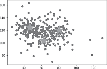
#For 2-D plot of the data points along with the centroids …
>>> fig = plt.figure()
>>> plt.scatter(X[:, 0], X[:, 1])
>>> plt.scatter(C[:, 0], C[:, 1], marker=’*’, s=1000)
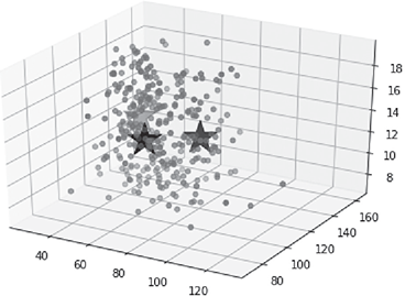
#For 3-D plot of the data points along with the centroids …
>>> fig = plt.figure()
>>> ax = Axes3D(fig)
>>> ax.scatter(X[:, 0], X[:, 1], X[:, 2])
>>> ax.scatter(C[:, 0], C[:, 1], C[:, 2], marker=’*’, c=’#050505’, s=1000)
Output Accuracy:
Centroids:
[[ 46.42903837 124.47018491 13.26250567]
[ 80.49567418 120.00557969 12.78133516]
[ 62.59438009 103.64870812 13.03697051]]
Silhouette width:
0.352350820437
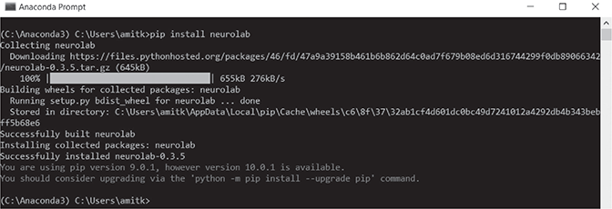
B.5.4 Neural network
For implementing neural network in Python, neurolab is a great option. It is a simple and powerful neural network library for Python. You can install neurolab by using the command below from the command prompt:
$ pip install neurolab
Please refer to the Figure B.9 for more details.
Copyright © 2018. Python Software Foundation
FIG. B.9 Installing neurolab from command prompt
Let’s first implement a single layer feed forward neural network. We can use the same set of data as provided as an example in Chapter 10, Section 10.6.2. The data is as below and output shown in Figure B.10.
This can summarized as
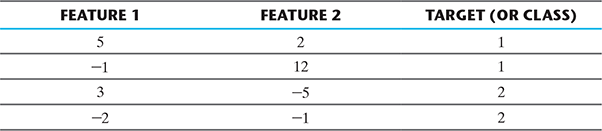
So let’s do the programming now.
>>> import neurolab as nl
>>> import matplotlib.pyplot as plt # Plot results
>>> input = [[5, 2], [-1, 12], [3, -5], [-2, -1]]
>>> target = [[1], [1], [2], [2]]
# Create single layer neural net with 2 inputs and 1 neuron
>>> net = nl.net.newp([[-2, 12],[1, 2]], 1) # Function newp is for implementing single layer perceptron …
>>> error = net.train(input, target, epochs=10, show=10, lr=0.1)
>>> plt.plot(error)
>>> plt.xlabel(‘Epoch number’)
>>> plt.ylabel(‘Train error’)
>>> plt.grid()
>>> plt.show()
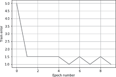
FIG. B.10 Epoch number vs. error in a single-layer NN
Next let’s implement a multi layer feed forward neural network. We can have multiple hidden layers in this case. In this case, we will use multi layer neural network as a regressor i.e. to predict a continuous variable. A set of 75 values of predictor variable is first generated within a specified range. The corresponding target values are generated using the equation y = 4x2 + 7.6 and normalized. Using these set of points, a multi layer neural network is trained. Then using the trained model, predictions are generated and compared with the actual data points generated from the regression function.
>>> import neurolab as nl
>>> import matplotlib.pyplot as plt
# Create train samples assuming minimum value = -2, maximum value = 2 and number of training points = 75
>>> minm_val = -2
>>> maxm_val = 2
>>> no_points = 75
>>> x = np.linspace(minm_val, maxm_val, no_points)
>>> y = 4*np.square(x) + 7.6
>>> y /= np.linalg.norm(y)
>>> input_data = x.reshape(no_points,1)
>>> target = y.reshape(no_points,1)
# Create network with 2 hidden layers - with 12 neurons in the first layer and 8 neurons in the second layer.
# Task is to predict the value, so the output layer will contain 1 neuron …
>>> net = nl.net.newff([[minm_val, maxm_val]],[12, 8, 1])
# Then the training algorithm is set to gradient descent …
>>> net.trainf = nl.train.train_gd
# Now do the real training
>>> error = net.train(input_data, target, epochs=2000, show=100, goal=0.01)
# Simulate network to generate prediction …
>>> output_data = net.sim(input_data)
>>> pred_val = output_data.reshape(no_points)
# Plotting the results …
>>> plt.figure()
>>> plt.plot(error)
>>> plt.xlabel(‘Epoch number’)
>>> plt.ylabel(‘Train error’)
>>> plt.grid()
>>> plt.show()
>>> x_dash = np.linspace(minm_val, maxm_val, no_points*2)
>>> y_dash = net.sim(x_dash.reshape(x_dash.size,1)).reshape(x_ dash.size)
>>> plt.figure()
>>> plt.plot(x_dash, y_dash, ‘.’, x, y, ‘+’, x, pred_val, ‘p’)
>>> plt.legend([‘Actual’, ‘Predicted’])
>>> plt.title(‘Actual vs predicted’)
>>> plt.show()
Output is presented in Figures B.11 and B.12.
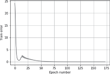
FIG. B.11 Epoch number vs. error in a multi layer NN
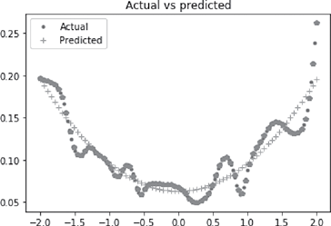
FIG. B.12 Actual vs. predicted in a multi layer NN
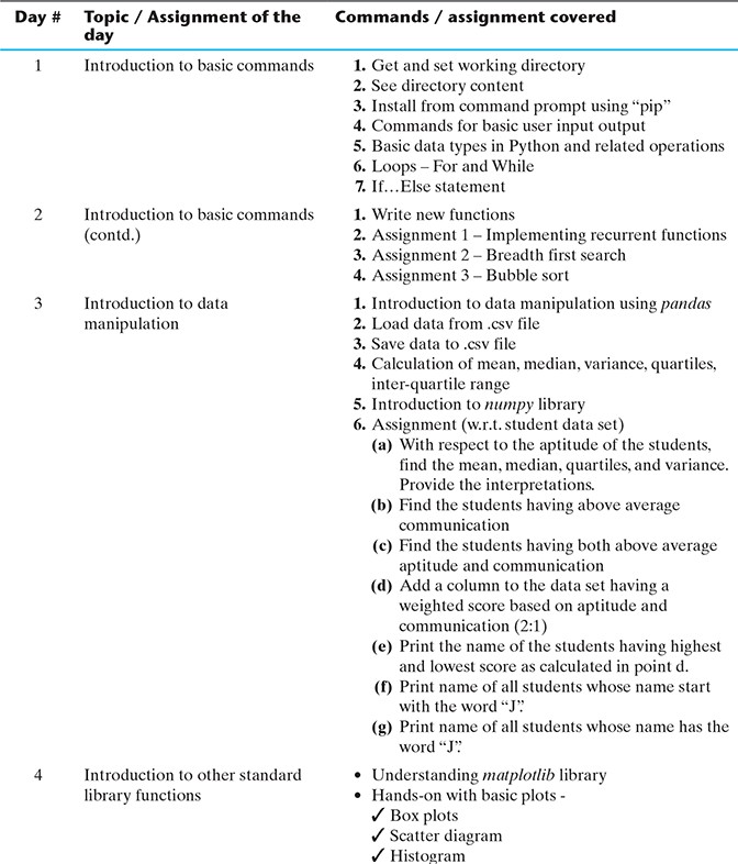
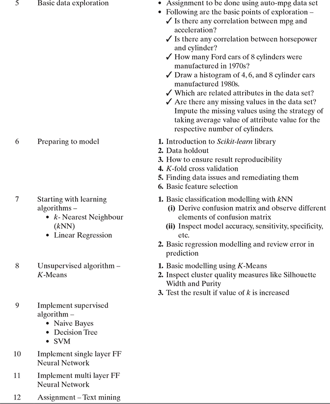
B.6 MACHINE LEARNING L AB USING PY THON – PROPOSED DAY-WISE SCHEDULE
Below is the proposed structure for a machine learning lab using Python.