
Chapter 9
Unsupervised Learning
OBJECTIVE OF THE CHAPTER :
We have discussed how to train our machines with past data on the basis of which they can learn, gain intelligence, and apply that intelligence on a new set of data. There are, however, situations when we do not have any prior knowledge of the data set we are working with, but we still want to discover interesting relationships among the attributes of the data or group the data in logical segments for easy analysis. The task of the machine is then to identify this knowledge without any prior training and that is the space of unsupervised learning. In this chapter, we will discuss how Clustering algorithms help in grouping data sets into logical segments and the association analysis which enables to identify a pattern or relationship of attributes within the data set. An interesting application of the association analysis is the Market Basket Analysis, which is used widely by retailers and advertisers across the globe.
9.1 INTRODUCTION
Unsupervised learning is a machine learning concept where the unlabelled and unclassified information is analysed to discover hidden knowledge. The algorithms work on the data without any prior training, but they are constructed in such a way that they can identify patterns, groupings, sorting order, and numerous other interesting knowledge from the set of data.
9.2 UNSUPERVISED VS SUPERVISED LEARNING
Till now, we have discussed about supervised learning where the aim was to predict the outcome variable Y on the basis of the feature set X1:X2:… Xn, and we discussed methods such as regression and classification for the same. We will now introduce the concept of unsupervised learning where the objective is to observe only the features X1:X2:… Xn; we are not going to predict any outcome variable, but rather our intention is to find out the association between the features or their grouping to understand the nature of the data. This analysis may reveal an interesting correlation between the features or a common behaviour within the subgroup of the data, which provides better understanding of the data.
In terms of statistics, a supervised learning algorithm will try to learn the probability of outcome Y for a particular input X, which is called the posterior probability. Unsupervised learning is closely related to density estimation in statistics. Here, every input and the corresponding targets are concatenated to create a new set of input such as {(X1, Y1), (X2, Y2),…, (Xn, Yn)}, which leads to a better understanding of the correlation of X and Y; this probability notation is called the joint probability.
Let us take an example of how unsupervised learning helps in pushing movie promotions to the correct group of people. In earlier days, movie promotions were blind push of the same data to all demography, such that everyone used to watch the same posters or trailers irrespective of their choice or preference. So, in most of the cases, the person watching the promotion or trailer would end up ignoring it, which leads to waste of effort and money on the promotion. But with the advent of smart devices and apps, there is now a huge database available to understand what type of movie is liked by what segment of the demography. Machine learning helps to find out the pattern or the repeated behaviour of the smaller groups/clusters within this database to provide the intelligence about liking or disliking of certain types of movies by different groups within the demography. So, by using this intelligence, the smart apps can push only the relevant movie promotions or trailers to the selected groups, which will significantly increase the chance of targeting the right interested person for the movie.
We will discuss two methods in this chapter for explaining the principle underlying unsupervised learning – Clustering and Association Analysis. Clustering is a broad class of methods used for discovering unknown subgroups in data, which is the most important concept in unsupervised learning. Another technique is Association Analysis which identifies a low-dimensional representation of the observations that can explain the variance and identify the association rule for the explanation.
9.3 APPLICATION OF UNSUPERVISED LEARNING
Because of its flexibility that it can work on uncategorized and unlabelled data, there are many domains where unsupervised learning finds its application. Few examples of such applications are as follows:
- Segmentation of target consumer populations by an advertisement consulting agency on the basis of few dimensions such as demography, financial data, purchasing habits, etc. so that the advertisers can reach their target consumers efficiently
- Anomaly or fraud detection in the banking sector by identifying the pattern of loan defaulters
- Image processing and image segmentation such as face recognition, expression identification, etc.
- Grouping of important characteristics in genes to identify important influencers in new areas of genetics
- Utilization by data scientists to reduce the dimensionalities in sample data to simplify modelling
- Document clustering and identifying potential labelling options
Today, unsupervised learning is used in many areas involving Artificial Intelligence (AI) and Machine Learning (ML). Chat bots, self-driven cars, and many more recent innovations are results of the combination of unsupervised and supervised learning.
So, in this chapter, we will cover two major aspects of unsupervised learning, namely Clustering which helps in segmentation of the set of objects into groups of similar objects and Association Analysis which is related to the identification of relationships among objects in a data set.
9.4 CLUSTERING
Clustering refers to a broad set of techniques for finding subgroups, or clusters, in a data set on the basis of the characteristics of the objects within that data set in such a manner that the objects within the group are similar (or related to each other) but are different from (or unrelated to) the objects from the other groups. The effectiveness of clustering depends on how similar or related the objects within a group are or how different or unrelated the objects in different groups are from each other. It is often domain specific to define what is meant by two objects to be similar or dissimilar and thus is an important aspect of the unsupervised machine learning task.
As an example, suppose we want to run some advertisements of a new movie for a countrywide promotional activity. We have data for the age, location, financial condition, and political stability of the people in different parts of the country. We may want to run a different type of campaign for the different parts grouped according to the data we have. Any logical grouping obtained by analysing the characteristics of the people will help us in driving the campaigns in a more targeted way. Clustering analysis can help in this activity by analysing different ways to group the set of people and arriving at different types of clusters.
There are many different fields where cluster analysis is used effectively, such as
- Text data mining: this includes tasks such as text categorization, text clustering, document summarization, concept extraction, sentiment analysis, and entity relation modelling
- Customer segmentation: creating clusters of customers on the basis of parameters such as demographics, financial conditions, buying habits, etc., which can be used by retailers and advertisers to promote their products in the correct segment
- Anomaly checking: checking of anomalous behaviours such as fraudulent bank transaction, unauthorized computer intrusion, suspicious movements on a radar scanner, etc.
- Data mining: simplify the data mining task by grouping a large number of features from an extremely large data set to make the analysis manageable
In this section, we will discuss the methods related to the machine learning task of clustering, which involves finding natural groupings of data. The focus will be on
- how clustering tasks differ from classification tasks and how clustering defines groups
- a classic and easy-to-understand clustering algorithm, namely k-means, which is used for clustering along with the k-medoids algorithm
- application of clustering in real-life scenarios
9.4.1 Clustering as a machine learning task
The primary driver of clustering knowledge is discovery rather than prediction, because we may not even know what we are looking for before starting the clustering analysis. So, clustering is defined as an unsupervised machine learning task that automatically divides the data into clusters or groups of similar items. The analysis achieves this without prior knowledge of the types of groups required and thus can provide an insight into the natural groupings within the data set. The primary guideline of clustering task is that the data inside a cluster should be very similar to each other but very different from those outside the cluster. We can assume that the definition of similarity might vary across applications, but the basic idea is always the same, that is, to create the group such that related elements are placed together. Using this principle, whenever a large set of diverse and varied data is presented for analysis, clustering enables to represent the data in a smaller number of groups. It helps to reduce the complexity and provides insight into patterns of relationships to generate meaningful and actionable structures within the data. The effectiveness of clustering is measured by the homogeneity within a group as well as the difference between distinct groups. See Figure 9.1 for reference.
From the above discussion, it may seem that through clustering, we are trying to label the objects with class labels. But clustering is somewhat different from the classification and numeric prediction discussed in supervised learning chapters. In each of these cases, the goal was to create a model that relates features to an outcome or to other features and the model identifies patterns within the data. In contrast, clustering creates new data. Unlabelled objects are given a cluster label which is inferred entirely from the relationship of attributes within the data.
Let us take an example. You were invited to take a session on Machine Learning in a reputed university for induction of their professors on the subject. Before you create the material for the session, you want to know the level of acquaintance of the professors on the subject so that the session is successful. But you do not want to ask the inviting university, but rather do some analysis on your own on the basis of the data available freely. As Machine Learning is the intersection of Statistics and Computer Science, you focused on identifying the professors from these two areas also. So, you searched the list of research publications of these professors from the internet, and by using the machine learning algorithm, you now want to group the papers and thus infer the expertise of the professors into three buckets – Statistics, Computer Science, and Machine Learning.
After plotting the number of publications of these professors in the two core areas, namely Statistics and Computer Science, you obtain a scatter plot as shown in Figure 9.2.
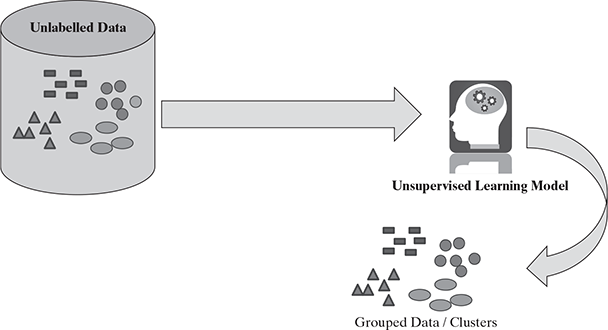
FIG. 9.1 Unsupervised learning – clustering
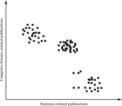
FIG. 9.2 Data set for the conference attendees
Some inferences that can be derived from the pattern analysis of the data is that there seems to be three groups or clusters emerging from the data. The pure statisticians have very less Computer Science-related papers, whereas the pure Computer Science professors have less number of statistics-related papers than Computer Science-related papers. There is a third cluster of professors who have published papers on both these areas and thus can be assumed to be the persons knowledgeable in machine learning concepts, as shown in Figure 9.3.
Thus, in the above problem, we used visual indication of logical grouping of data to identify a pattern or cluster and labelled the data in three different clusters. The main driver for our clustering was the closeness of the points to each other to form a group. The clustering algorithm uses a very similar approach to measure how closely the data points are related and decides whether they can be labelled as a homogeneous group. In the next section, we will discuss few important algorithms for clustering.
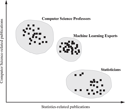
FIG. 9.3 Clusters for the conference attendees
9.4.2 Different types of clustering techniques
The major clustering techniques are
- Partitioning methods,
- Hierarchical methods, and
- Density-based methods.
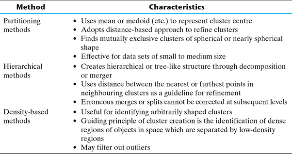
Their approach towards creating the clusters, way to measure the quality of the clusters, and applicability are different. Table 9.1 summarizes the main characteristics of each method for each reference.
Table 9.1 Different Clustering Methods
We will discuss each of these methods and their related techniques in details in the following sections.
9.4.3 Partitioning methods
Two of the most important algorithms for partitioning-based clustering are k-means and k-medoid. In the k-means algorithm, the centroid of the prototype is identified for clustering, which is normally the mean of a group of points. Similarly, the k-medoid algorithm identifies the medoid which is the most representative point for a group of points. We can also infer that in most cases, the centroid does not correspond to an actual data point, whereas medoid is always an actual data point. Let us discuss both these algorithms in detail.
9.4.3.1 K-means - A centroid-based technique
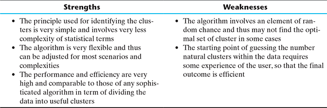
This is one of the oldest and most popularly used algorithm for clustering. The basic principles used by this algorithm also serves as the basis for other more sophisticated and complex algorithms. Table 9.2 provides the strengths and weaknesses of this algorithm.
The principle of the k-means algorithm is to assign each of the ‘n’ data points to one of the K clusters where ‘K’ is a user-defined parameter as the number of clusters desired. The objective is to maximize the homogeneity within the clusters and also to maximize the differences between the clusters. The homogeneity and differences are measured in terms of the distance between the objects or points in the data set.
Algorithm 9.1 shows the simple algorithm of K-means
Step 1: Select K points in the data space and mark them as initial centroids
loop
Step 2: Assign each point in the data space to the nearest centroid to form K clusters
Step 3: Measure the distance of each point in the cluster from the centroid
Step 4: Calculate the Sum of Squared Error (SSE) to measure the quality of the clusters (described later in this chapter)
Step 5: Identify the new centroid of each cluster on the basis of distance between points
Step 6: Repeat Steps 2 to 5 to refine until centroids do not change
end loop
Table 9.2 Strengths and Weaknesses of K-means
Let us understand this algorithm with an example. In Figure 9.4, we have certain set of data points, and we will apply the k-means algorithm to find out the clusters generated from this data set. Let us fix K = 4, implying that we want to create four clusters out of this data set. As the first step, we assign four random points from the data set as the centroids, as represented by the * signs, and we assign the data points to the nearest centroid to create four clusters. In the second step, on the basis of the distance of the points from the corresponding centroids, the centroids are updated and points are reassigned to the updated centroids. After three iterations, we found that the centroids are not moving as there is no scope for refinement, and thus, the k-means algorithm will terminate. This provides us the most logical four groupings or cluster of the data sets where the homogeneity within the groups is highest and difference between the groups is maximum.
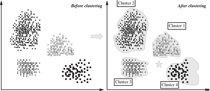
FIG. 9.4 Clustering concept – before and after clustering
Choosing appropriate number of clusters
One of the most important success factors in arriving at correct clustering is to start with the correct number of cluster assumptions. Different numbers of starting cluster lead to completely different types of data split. It will always help if we have some prior knowledge about the number of clusters and we start our k-means algorithm with that prior knowledge. For example, if we are clustering the data of the students of a university, it is always better to start with the number of departments in that university. Sometimes, the business needs or resource limitations drive the number of required clusters. For example, if a movie maker wants to cluster the movies on the basis of combination of two parameters – budget of the movie: high or low, and casting of the movie: star or non-star, then there are 4 possible combinations, and thus, there can be four clusters to split the data.
For a small data set, sometimes a rule of thumb that is followed is
which means that K is set as the square root of n/2 for a data set of n examples. But unfortunately, this thumb rule does not work well for large data sets. There are several statistical methods to arrive at the suitable number of clusters.
Elbow method
This method tries to measure the homogeneity or heterogeneity within the cluster and for various values of ‘K’ and helps in arriving at the optimal ‘K’. From Figure 9.5, we can see the homogeneity will increase or heterogeneity will decrease with increasing ‘K’ as the number of data points inside each cluster reduces with this increase. But these iterations take significant computation effort, and after a certain point, the increase in homogeneity benefit is no longer in accordance with the investment required to achieve it, as is evident from the figure. This point is known as the elbow point, and the ‘K’ value at this point produces the optimal clustering performance. There are a large number of algorithms to calculate the homogeneity and heterogeneity of the clusters, which are not discussed in this book.
Choosing the initial centroids
Another key step for the k-means algorithm is to choose the initial centroids properly. One common practice is to choose random points in the data space on the basis of the number of cluster requirement and refine the points as we move into the iterations. But this often leads to higher squared error in the final clustering, thus resulting in sub-optimal clustering solution. The assumption for selecting random centroids is that multiple subsequent runs will minimize the SSE and identify the optimal clusters. But this is often not true on the basis of the spread of the data set and the number of clusters sought. So, one effective approach is to employ the hierarchical clustering technique on sample points from the data set and then arrive at sample K clusters. The centroids of these initial K clusters are used as the initial centroids. This approach is practical when the data set has small number of points and K is relatively small compared to the data points. There are procedures such as bisecting k-means and use of post-processing to fix initial clustering issues; these procedures can produce better quality initial centroids and thus better SSE for the final clusters.
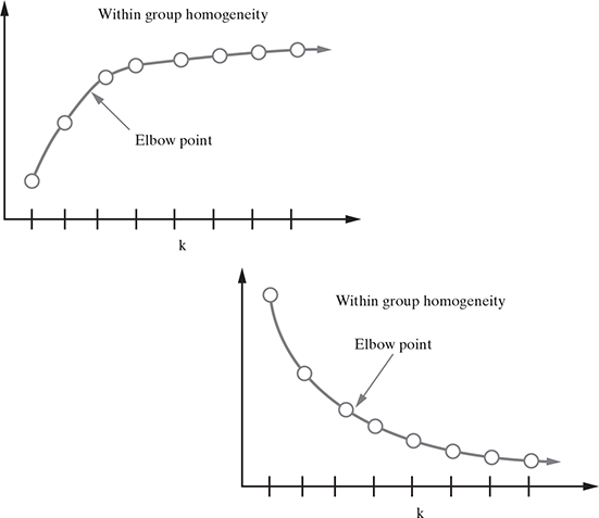
FIG. 9.5 Elbow point to determine the appropriate number of clusters
Recomputing cluster centroids
We discussed in the k-means algorithm that the iterative step is to recalculate the centroids of the data set after each iteration. The proximities of the data points from each other within a cluster is measured to minimize the distances. The distance of the data point from its nearest centroid can also be calculated to minimize the distances to arrive at the refined centroid. The Euclidean distance between two data points is measured as follows:
Using this function, the distance between the example data and its nearest centroid and the objective is calculated to minimize this distance. The measure of quality of clustering uses the SSE technique. The formula used is as follows:
where dist() calculates the Euclidean distance between the centroid ci of the cluster Ci and the data points x in the cluster. The summation of such distances over all the ‘K’ clusters gives the total sum of squared error. As you can understand, the lower the SSE for a clustering solution, the better is the representative position of the centroid. Thus, in our clustering algorithm in Algorithm 9.1, the recomputation of the centroid involves calculating the SSE of each new centroid and arriving at the optimal centroid identification. After the centroids are repositioned, the data points nearest to the centroids are assigned to form the refined clusters. It is observed that the centroid that minimizes the SSE of the cluster is its mean. One limitation of the squared error method is that in the case of presence of outliers in the data set, the squared error can distort the mean value of the clusters.
Let us use this understanding to identify the cluster step for the data set in Figure 9.6. Assume that the number of cluster requirement, K = 4. We will randomly select four cluster centroids as indicated by four different colours in Figure 9.7.
Now, on the basis of the proximity of the data points in this data set to the centroids, we partition the data set into four segments as represented by dashed lines in Figure 9.8. This diagram is called Voronoi diagram which creates the boundaries of the clusters. We got the initial four clusters, namely C 1 , C 2 , C 3 , and C 4 , created by the dashed lines from the vertex of the clusters, which is the point with the maximal distance from the centre of the clusters. It is now easy to understand the areas covered by each cluster and the data points within each cluster through this representation.
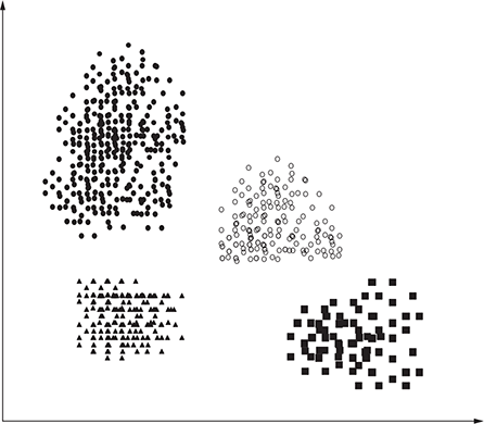
FIG. 9.6 Clustering of data set
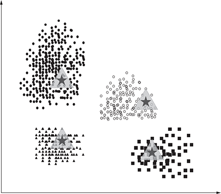
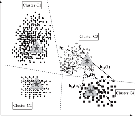
FIG. 9.8 Iteration 1: Four clusters and distance of points from the centroids
The next step is to calculate the SSE of this clustering and update the position of the centroids. We can also proceed by our understanding that the new centroid should be the mean of the data points in the respective clusters. The distances of the data points currently marked as Cluster C3 from the centroid of cluster C3 are marked as ai1 , ai2 ,…, ain in the figure and those determine the homogeneity within cluster C3. On the other hand, the distances of data points of cluster C4 from the centroid of cluster C3 determine the heterogeneity among these two different clusters. Our aim is to minimize the homogeneity within the clusters and maximize the heterogeneity among the different clusters. So, the revised centroids are as shown in Figure 9.9.
We can also find out that the cluster boundaries are refined on the basis of the new centroids and the identification of the nearest centroids for the data points and reassigning them to the new centroids. The new points reclaimed by each cluster are shown in the diagram.
The k-means algorithm continues with the update of the centroid according to the new cluster and reassignment of the points, until no more data points are changed due to the centroid shift. At this point, the algorithm stops. Figure 9.10 shows the final clustering of the data set we used. The complexity of the k-means algorithm is O ( nKt ), where ‘ n ’ is the total number of data points or objects in the data set, K is the number of clusters, and ‘ t ’ is the number of iterations. Normally, ‘ K ’ and ‘ t ’ are kept much smaller than ‘ n ’, and thus, the k-means method is relatively scalable and efficient in processing large data sets.
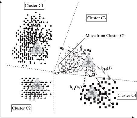
FIG. 9.9 Iteration 2: Centroids recomputed and points redistributed among the clusters according to the nearest centroid
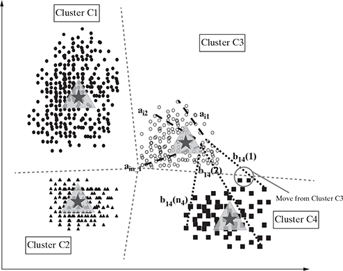
FIG. 9.10 Iteration 3: Final cluster arrangement: Centroids recomputed and points redistributed among the clusters according to the nearest centroid
Points to Ponder:
Because of the distance-based approach from the centroid to all points in the data set, the k-means method may not always converge to the global optimum and often terminates at a local optimum. The result of the clustering largely depends on the initial random selection of cluster centres.
k-means often produce local optimum and not global optimum. Also, the result depends on the initial selection of random cluster centroids. It is a common practice to run the k-means algorithm multiple times with different cluster centres to identify the optimal clusters. The necessity to set the initial ‘K’ values is also perceived as a disadvantage of the k-means algorithm. There are methods to overcome this problem, such as defining a range for ‘K’ and then comparing the results of clustering with those different ‘K’ values to arrive at the best possible cluster. The ways to improve cluster performance is an area of further study, and many different techniques are employed to achieve that. This is out of scope of this book but can be pursued for advanced machine learning studies.
Note:
Clustering is often used as the first step of identifying the subgroups within a unlabeled set of data which then is used for classifying the new observed data. At the beginning we are not clear about the pattern or classes that exist within the unlabeled data set. By using the clustering algorithm at that stage we find out the groups of similar objects within the data set and form sub-groups and classes. Later when a new object is observed, then using the classification algorithms we try to place that into one of the sub-groups identified in the earlier stage. Let’s take an example. We are running a software testing activity and we identified a set of defects in the software. For easy allocation of these defects to different developer groups, the team is trying to identify similar groups of defects. Often text analytics is used as the guiding principle for identifying this similarity. Suppose there are 4 sub-groups of defects identified, namely, GUI related defects, Business logic related defects, Missing requirement defects and Database related defects. Based on this grouping, the team identified the developers to whom the defects should be sent for fixing. As the testing continues, there are new defects getting created. We have the categories of defects identified now and thus the team can use classification algorithms to assign the new defect to one of the 4 identified groups or classes which will make it easy to identify the developer who should be fixing it.
9.4.4 K-Medoids: a representative object-based technique
As discussed earlier, the k-means algorithm is sensitive to outliers in the data set and inadvertently produces skewed clusters when the means of the data points are used as centroids. Let us take an example of eight data points, and for simplicity, we can consider them to be 1-D data with values 1, 2, 3, 5, 9, 10, 11, and 25. Point 25 is the outlier, and it affects the cluster formation negatively when the mean of the points is considered as centroids.
With K = 2, the initial clusters we arrived at are {1, 2, 3, 6} and {9, 10, 11, 25}.
The mean of the cluster ![]()
and the mean of the cluster ![]()
So, the SSE within the clusters is
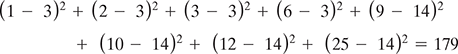
If we compare this with the cluster {1, 2, 3, 6, 9} and {10, 11, 25},
the mean of the cluster ![]()
and the mean of the cluster ![]()
So, the SSE within the clusters is
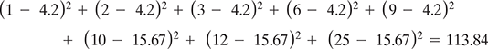
Because the SSE of the second clustering is lower, k-means tend to put point 9 in the same cluster with 1, 2, 3, and 6 though the point is logically nearer to points 10 and 11. This skewedness is introduced due to the outlier point 25, which shifts the mean away from the centre of the cluster.
k-medoids provides a solution to this problem. Instead of considering the mean of the data points in the cluster, k-medoids considers k representative data points from the existing points in the data set as the centre of the clusters. It then assigns the data points according to their distance from these centres to form k clusters. Note that the medoids in this case are actual data points or objects from the data set and not an imaginary point as in the case when the mean of the data sets within cluster is used as the centroid in the k-means technique. The SSE is calculated as
where oi is the representative point or object of cluster Ci.
Thus, the k-medoids method groups n objects in k clusters by minimizing the SSE. Because of the use of medoids from the actual representative data points, k-medoids is less influenced by the outliers in the data. One of the practical implementation of the k-medoids principle is the Partitioning Around Medoids (PAM) algorithm. Refer to Algorithm 2 table:
Algorithm 2: PAM
Step 1: Randomly choose k points in the data set as the initial representative points
loop
Step 2: Assign each of the remaining points to the cluster which has the nearest representative point
Step 3: Randomly select a non-representative point or in each cluster
Step 4: Swap the representative point oj with or and compute the new SSE after swapping
Step 5: If SSEnew < SSEold, then swap oj with or to form the new set of k representative objects;
Step 6: Refine the k clusters on the basis of the nearest representative point. Logic continues until there is no change
end loop
In this algorithm, we replaced the current representative object with a non-representative object and checked if it improves the quality of clustering. In the iterative process, all possible replacements are attempted until the quality of clusters no longer improves.
If o1,…, ok are the current set of representative objects or medoids and there is a non-representative object or, then to determine whether or is a good replacement of oj (1 ≤ j ≤ k), the distance of each object x is calculated from its nearest medoid from the set {o1, o2,…, oj−1, or, oj+1,…, ok} and the SSE is calculated. If the SSE after replacing oj with or decreases, it means that or represents the cluster better than oj, and the data points in the set are reassigned according to the nearest medoids now.
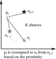
FIG. 9.11 PAM algorithm: Reassignment of points to different clusters
As shown in Figure 9.11, point pi was belonging to the cluster with medoid oj+1 in the first iteration, but after oj was replaced by or, it was found that pi is nearest to the new random medoid and thus gets assigned to it. In this way, the clusters get refined after each medoid is replaced with a new non-representative medoid. Each time a reassignment is done, the SSE based on the new medoid is calculated. The difference between the SSE before and after the swap indicates whether or not the replacement is improving the quality of the clustering by bringing the most similar points together.
Points to Ponder:
k-medoids methods like PAM works well for small set of data, but they are not scalable for large set of data because of computational overhead. A sample-based technique is used in the case of large data set where the sample should be a good representative of the whole data set.
Though the k-medoids algorithm provides an effective way to eliminate the noise or outliers in the data set, which was the problem in the k-means algorithm, it is expensive in terms of calculations. The complexity of each iteration in the k-medoids algorithm is O(k(n - k)2). For large value of ‘n’ and ‘k’, this calculation becomes much costlier than that of the k-means algorithm.
9.4.5 Hierarchical clustering
Till now, we have discussed the various methods for partitioning the data into different clusters. But there are situations when the data needs to be partitioned into groups at different levels such as in a hierarchy. The hierarchical clustering methods are used to group the data into hierarchy or tree-like structure. For example, in a machine learning problem of organizing employees of a university in different departments, first the employees are grouped under the different departments in the university, and then within each department, the employees can be grouped according to their roles such as professors, assistant professors, supervisors, lab assistants, etc. This creates a hierarchical structure of the employee data and eases visualization and analysis. Similarly, there may be a data set which has an underlying hierarchy structure that we want to discover and we can use the hierarchical clustering methods to achieve that.
There are two main hierarchical clustering methods: agglomerative clustering and divisive clustering. Agglomerative clustering is a bottom-up technique which starts with individual objects as clusters and then iteratively merges them to form larger clusters. On the other hand, the divisive method starts with one cluster with all given objects and then splits it iteratively to form smaller clusters. See Figure 9.12.
The agglomerative hierarchical clustering method uses the bottom-up strategy. It starts with each object forming its own cluster and then iteratively merges the clusters according to their similarity to form larger clusters. It terminates either when a certain clustering condition imposed by the user is achieved or all the clusters merge into a single cluster.
The divisive hierarchical clustering method uses a top-down strategy. The starting point is the largest cluster with all the objects in it, and then, it is split recursively to form smaller and smaller clusters, thus forming the hierarchy. The end of iterations is achieved when the objects in the final clusters are sufficiently homogeneous to each other or the final clusters contain only one object or the user-defined clustering condition is achieved.
In both these cases, it is important to select the split and merger points carefully, because the subsequent splits or mergers will use the result of the previous ones and there is no option to perform any object swapping between the clusters or rectify the decisions made in previous steps, which may result in poor clustering quality at the end.
A dendrogram is a commonly used tree structure representation of step-by-step creation of hierarchical clustering. It shows how the clusters are merged iteratively (in the case of agglomerative clustering) or split iteratively (in the case of divisive clustering) to arrive at the optimal clustering solution. Figure 9.13 shows a dendro-gram with four levels and how the objects are merged or split at each level to arrive at the hierarchical clustering.
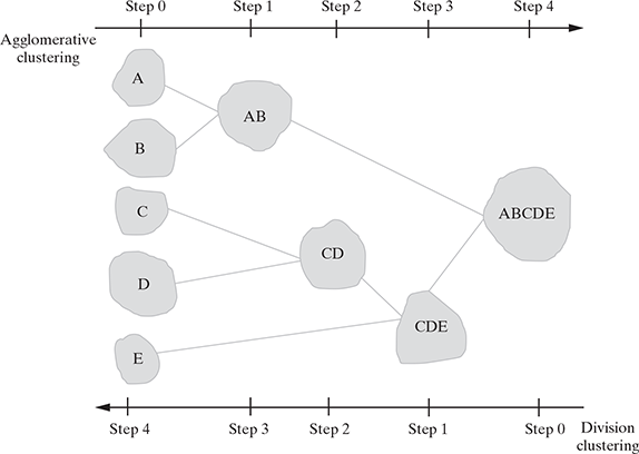
FIG. 9.12 Agglomerative and divisive hierarchical clustering
One of the core measures of proximities between clusters is the distance between them. There are four standard methods to measure the distance between clusters:
Let Ci and Cj be the two clusters with ni and nj respectively. pi and pj represents the points in clusters Ci and Cj respectively. We will denote the mean of cluster Ci as mi.
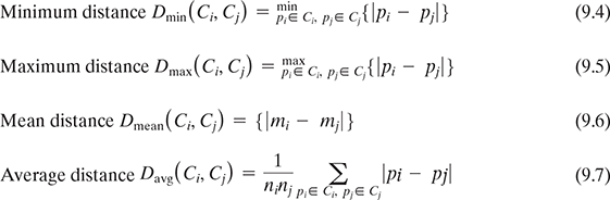
Refer to Figure 9.14 for understanding the concept of these distances.
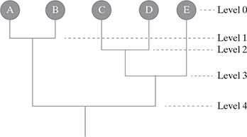
FIG. 9.13 Dendrogram representation of hierarchical clustering
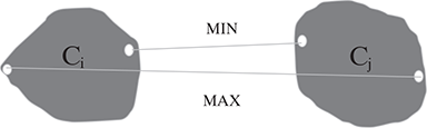
FIG. 9.14 Distance measure in algorithmic methods
Often the distance measure is used to decide when to terminate the clustering algorithm. For example, in an agglomerative clustering, the merging iterations may be stopped once the MIN distance between two neighbouring clusters becomes less than the user-defined threshold. So, when an algorithm uses the minimum distance Dmin to measure the distance between the clusters, then it is referred to as nearest neighbour clustering algorithm, and if the decision to stop the algorithm is based on a user-defined limit on Dmin, then it is called single linkage algorithm.
On the other hand, when an algorithm uses the maximum distance Dmax to measure the distance between the clusters, then it is referred to as furthest neighbour clustering algorithm, and if the decision to stop the algorithm is based on a user-defined limit on Dmax then it is called complete linkage algorithm.
As minimum and maximum measures provide two extreme options to measure distance between the clusters, they are prone to the outliers and noisy data. Instead, the use of mean and average distance helps in avoiding such problem and provides more consistent results.
9.4.6 Density-based methods - DBSCAN
You might have noticed that when we used the partitioning and hierarchical clustering methods, the resulting clusters are spherical or nearly spherical in nature. In the case of the other shaped clusters such as S-shaped or uneven shaped clusters, the above two types of method do not provide accurate results. The density-based clustering approach provides a solution to identify clusters of arbitrary shapes. The principle is based on identifying the dense area and sparse area within the data set and then run the clustering algorithm. DBSCAN is one of the popular density-based algorithm which creates clusters by using connected regions with high density.
9.5 FINDING PATTERN USING ASSOCIATION RULE
Association rule presents a methodology that is useful for identifying interesting relationships hidden in large data sets. It is also known as association analysis, and the discovered relationships can be represented in the form of association rules comprising a set of frequent items. A common application of this analysis is the Market Basket Analysis that retailers use for cross-selling of their products. For example, every large grocery store accumulates a large volume of data about the buying pattern of the customers. On the basis of the items purchased together, the retailers can push some cross-selling either by placing the items bought together in adjacent areas or creating some combo offer with those different product types. The below association rule signifies that people who have bought bread and milk have often bought egg also; so, for the retailer, it makes sense that these items are placed together for new opportunities for cross-selling.
The application of association analysis is also widespread in other domains such as bioinformatics, medical diagnosis, scientific data analysis, and web data mining. For example, by discovering the interesting relationship between food habit and patients developing breast cancer, a new cancer prevention mechanism can be found which will benefit thousands of people in the world. In this book, we will mainly illustrate the analysis techniques by using the market basket example, but it can be used more widely across domains to identify association among items in transactional data. The huge pool of data generated everyday through tracked transactions such as barcode scanner, online purchase, and inventory tracking systems has enabled for machine learning systems to learn from this wealth of data. We will discuss the methods for finding useful associations in large databases by using simple statistical performance measures while managing the peculiarities of working with such transactional data. One significant challenge in working with the large volume of data is that it may be computationally very expensive to discover patterns from such data. Moreover, there may be cases when some of the associations occurred by chance, which can lead to potentially false knowledge. While discussing the association analysis, we will discuss both these points.
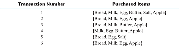
We will use the transaction data in the table below for our examples of association analysis. This simplified version of the market basket data will show how the association rules can be effectively used for the market basket analysis.
9.5.1 Definition of common terms
Let us understand few common terminologies used in association analysis.
9.5.1.1 Itemset
One or more items are grouped together and are surrounded by brackets to indicate that they form a set, or more specifically, an itemset that appears in the data with some regularity. For example, in Table 9.3, {Bread, Milk, Egg} can be grouped together to form an itemset as those are frequently bought together. To generalize this concept, if I = {i1, i2,…, in} are the items in a market basket data and T = {t1, t2,…, tn} are the set of all the transactions, then each transaction ti contains a subset of items from I. A collection of zero or more items is called an itemset. A null itemset is the one which does not contain any item. In the association analysis, an itemset is called k-itemset if it contains k number of items. Thus, the itemset {Bread, Milk, Egg} is a three-itemset.
Table 9.3 Market Basket Transaction Data
9.5.1.2 Support count
Support count denotes the number of transactions in which a particular itemset is present. This is a very important property of an itemset as it denotes the frequency of occurrence for the itemset. This is expressed as
where |{}| denotes the number of elements in a set
In Table 9.3, the itemset {Bread, Milk, Egg} occurs together three times and thus have a support count of 3.
9.5.2 Association rule
The result of the market basket analysis is expressed as a set of association rules that specify patterns of relationships among items. A typical rule might be expressed as{Bread, Milk}→{Egg}, which denotes that if Bread and Milk are purchased, then Egg is also likely to be purchased. Thus, association rules are learned from subsets of itemsets. For example, the preceding rule was identified from the set of {Bread, Milk, Egg}.
It should be noted that an association rule is an expression of X → Y where X and Y are disjoint itemsets, i.e. X ∩ Y = 0.
Support and confidence are the two concepts that are used for measuring the strength of an association rule. Support denotes how often a rule is applicable to a given data set. Confidence indicates how often the items in Y appear in transactions that contain X in a total transaction of N. Confidence denotes the predictive power or accuracy of the rule. So, the mathematical expressions are
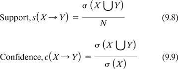
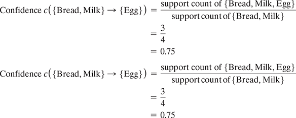
In our data set 9.3, if we consider the association rule {Bread, Milk} → {Egg}, then from the above formula
It is important to understand the role of support and confidence in the association analysis. A low support may indicate that the rule has occurred by chance. Also, from its application perspective, this rule may not be a very attractive business investment as the items are seldom bought together by the customers. Thus, support can provide the intelligence of identifying the most interesting rules for analysis.
Similarly, confidence provides the measurement for reliability of the inference of a rule. Higher confidence of a rule X → Y denotes more likelihood of to be present in transactions that contain X as it is the estimate of the conditional probability of Y given X.
Also, understand that the confidence of X leading to Y is not the same as the confidence of Y leading to X. In our example, confidence of {Bread, Milk} → {Egg} = 0.75 but confidence of ![]() Here, the rule {Bread, Milk} → {Egg} is the strong rule.
Here, the rule {Bread, Milk} → {Egg} is the strong rule.
Association rules were developed in the context of Big Data and data science and are not used for prediction. They are used for unsupervised knowledge discovery in large databases, unlike the classification and numeric prediction algorithms. Still we will find that association rule learners are closely related to and share many features of the classification rule learners. As association rule learners are unsupervised, there is no need for the algorithm to be trained; this means that no prior labelling of the data is required. The programme is simply run on a data set in the hope that interesting associations are found.
Obviously, the downside is that there is not an easy way to objectively measure the performance of a rule learner, aside from evaluating them for qualitative usefulness. Also, note that the association rule analysis is used to search for interesting connections among a very large number of variables. Though human beings are capable of such insight quite intuitively, sometimes it requires expert-level knowledge or a great deal of experience to achieve the performance of a rule-learning algorithm. Additionally, some data may be too large or complex for humans to decipher and analyse so easily.
9.5.3 The apriori algorithm for association rule learning
As discussed earlier, the main challenge of discovering an association rule and learning from it is the large volume of transactional data and the related complexity. Because of the variation of features in transactional data, the number of feature sets within a data set usually becomes very large. This leads to the problem of handling a very large number of itemsets, which grows exponentially with the number of features. If there are k items which may or may not be part of an itemset, then there is 2k ways of creating itemsets with those items. For example, if a seller is dealing with 100 different items, then the learner need to evaluate 2100 = 1 × e30 itemsets for arriving at the rule, which is computationally impossible. So, it is important to filter out the most important (and thus manageable in size) itemsets and use the resources on those to arrive at the reasonably efficient association rules.
The first step for us is to decide the minimum support and minimum confidence of the association rules. From a set of transaction T, let us assume that we will find out all the rules that have support ≥ minS and confidence ≥ minC, where minS and minC are the support and confidence thresholds, respectively, for the rules to be considered acceptable. Now, even if we put the minS = 20% and minC = 50%, it is seen that more than 80% of the rules are discarded; this means that a large portion of the computational efforts could have been avoided if the itemsets for consideration were first pruned and the itemsets which cannot generate association rules with reasonable support and confidence were removed. The approach to achieve this goal is discussed below.
Step 1: decouple the support and confidence requirements. According to formula 9.8, the support of the rule X → Y is dependent only on the support of its corresponding itemsets. For example, all the below rules have the same support as their itemsets are the same {Bread, Milk, Egg}:
- {Bread, Milk} → {Egg}
- {Bread, Egg} → {Milk}
- {Egg, Milk} → {Bread}
- {Bread} → {Egg, Milk}
- {Milk} → {Bread, Egg}
- {Egg} → {Bread, Milk}
So, the same treatment can be applied to this association rule on the basis of the frequency of the itemset. In this case, if the itemset {Bread, Milk, Egg} is rare in the basket transactions, then all these six rules can be discarded without computing their individual support and confidence values. This identifies some important strategies for arriving at the association rules:
- Generate Frequent Itemset: Once the minS is set for a particular assignment, identify all the itemsets that satisfy minS. These itemsets are called frequent itemsets.
- Generate Rules: From the frequent itemsets found in the previous step, discover all the high confidence rules. These are called strong rules.
Please note that the computation requirement for identifying frequent itemsets is more intense than the rule generation. So, different techniques have been evolved to optimize the performance for frequent itemset generation as well as rule discovery as discussed in the next section.
9.5.4 Build the apriori principle rules
One of the most widely used algorithm to reduce the number of itemsets to search for the association rule is known as Apriori. It has proven to be successful in simplifying the association rule learning to a great extent. The principle got its name from the fact that the algorithm utilizes a simple prior belief (i.e. a priori) about the properties of frequent itemsets:
If an itemset is frequent, then all of its subsets must also be frequent.
This principle significantly restricts the number of itemsets to be searched for rule generation. For example, if in a market basket analysis, it is found that an item like ‘Salt’ is not so frequently bought along with the breakfast items, then it is fine to remove all the itemsets containing salt for rule generation as their contribution to the support and confidence of the rule will be insignificant.
The converse also holds true:
If an itemset is frequent, then all the supersets must be frequent too.
These are very powerful principles which help in pruning the exponential search space based on the support measure and is known as support-based pruning. The key property of the support measure used here is that the support for an itemset never exceeds the support for its subsets. This is also known as the anti-monotone property of the support measure.
Let us use the transaction data in Table 9.3 to illustrate the Apriori principle and its use. From the full itemset of six items {Bread, Milk, Egg, Butter, Salt, Apple}, there are 26 ways to create baskets or itemsets (including the null itemset) as shown in Figure 9.15:
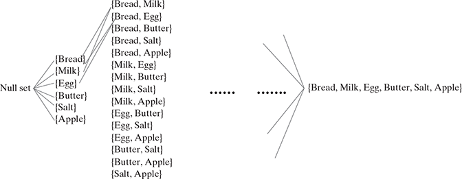
FIG. 9.15 Sixty-four ways to create itemsets from 6 items
Without applying any filtering logic, the brute-force approach would involve calculating the support count for each itemset in Figure 9.16. Thus, by comparing each item in the generated itemset with the actual transactions mentioned in Table 9.3, we can determine the support count of the itemset. For example, if {Bread, Milk} is present in any transactions in Table 9.3, then its support count will be incremented by 1. As we can understand, this is a very computation heavy activity, and as discussed earlier, many of the computations may get wasted at a later point of time because some itemsets will be found to be infrequent in the transactions. To get an idea of the total computations to be done, the number of comparisons to be done is T × N × L, where T is the number of transactions (6 in our case), N is the number of candidate itemsets (64 in our case), and L is the maximum transaction width (6 in our case).
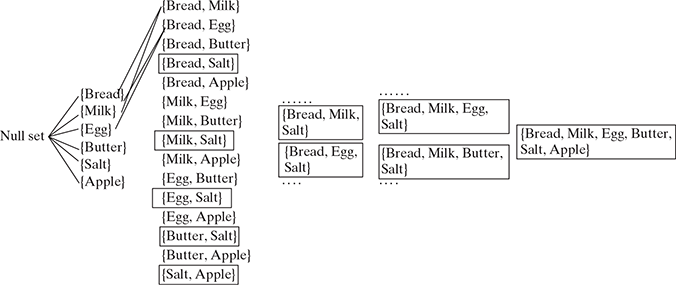
FIG. 9.16 Discarding the itemsets consisting of Salt
Let us apply the Apriori principle on this data set to reduce the number of candidate itemsets (N). We could identify from the transaction Table 9.3 that Salt is an infrequent item. So, by applying the Apriori principle, we can say that all the itemsets which are superset of Salt will be infrequent and thus can be discarded from comparison to discover the association rule as shown in Figure 9.16.
This approach reduces the computation effort for a good number of itemsets and will make our search process more efficient. Thus, in each such iteration, we can determine the support count of each itemset, and on the basis of the min support value fixed for our analysis, any itemset in the hierarchy that does not meet the min support criteria can be discarded to make the rule generation faster and easier.
To generalize the example in order to build a set of rules with the Apriori principle, we will use the Apriori principle that states that all subsets of a frequent itemset must also be frequent. In other words, if {X, Y} is frequent, then both {X} and {Y} must be frequent. Also by definition, the support metric indicates how frequently an itemset appears in the data. Thus, if we know that {X} does not meet a desired support threshold, there is no reason to consider {X, Y} or any itemset containing {X}; it cannot possibly be frequent.
This logic of the Apriori algorithm excludes potential association rules prior to actually evaluating them. The actual process of creating rules involves two phases:
- Identifying all itemsets that meet a minimum support threshold set for the analysis
- Creating rules from these itemsets that meet a minimum confidence threshold which identifies the strong rules
The first phase involves multiple iterations where each successive iteration requires evaluating the support of storing a set of increasingly large itemsets. For instance, iteration 1 evaluates the set of one-item itemsets (one-itemsets), iteration 2 involves evaluating the two-itemsets, etc.. The result of each iteration N is a set of all N-itemsets that meet the minimum support threshold. Normally, all the itemsets from iteration N are combined in order to generate candidate itemsets for evaluation in iteration N + 1, but by applying the Apriori principle, we can eliminate some of them even before the next iteration starts. If {X}, {Y}, and {Z} are frequent in iteration 1 while {W} is not frequent, then iteration 2 will consider only {X, Y}, {X, Z}, and {Y, Z}. We can see that the algorithm needs to evaluate only three itemsets rather than the six that would have been evaluated if sets containing W had not been eliminated by apriori.
By continuing with the iterations, let us assume that during iteration 2, it is discovered that {X, Y} and {Y, Z} are frequent, but {X, Z} is not. Although iteration 3 would normally begin by evaluating the support for {X, Y, Z}, this step need not occur at all. The Apriori principle states that {X, Y, Z} cannot be frequent, because the subset {X, Z} is not. Therefore, in iteration 3, the algorithm may stop as no new itemset can be generated.
Once we identify the qualifying itemsets for analysis, the second phase of the Apriori algorithm begins. For the given set of frequent itemsets, association rules are generated from all possible subsets. For example, {X, Y} would result in candidate rules for {X} → {Y} and {Y} → {X}. These rules are evaluated against a minimum confidence threshold, and any rule that does not meet the desired confidence level is eliminated, thus finally yielding the set of strong rules.
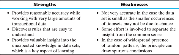
Though the Apriori principle is widely used in the market basket analysis and other applications of association rule help in the discovery of new relationship among objects, there are certain strengths and weaknesses we need to keep in mind before employing it over the target data set:
9.6 SUMMARY
- Unsupervised learning is a machine learning concept where the unlabelled and unclassified information is analysed to discover hidden knowledge. The algorithm works on the data without any prior training, but they are constructed in such a way that they can identify patterns, groupings, sorting order, and numerous other interesting knowledge from the set of data.
- Clustering refers to a broad set of techniques for finding subgroups, or clusters, in a data set based on the characteristics of the objects within the data set itself in such a manner that the objects within the group are similar (or related to each other) but are different from (or unrelated to) the objects from the other groups.
- The major clustering techniques are classified in three board categories
- Partitioning methods,
- Hierarchical methods, and
- Density-based methods.
- k-means and k-medoids are the most popular partitioning techniques.
- The principle of k-means algorithm is to assign each of the n data points to one of the k clusters, where k is a user-defined parameter as the number of clusters desired. The objective is to maximize the homogeneity within the clusters and to maximize the differences between the clusters. The homogeneity and differences are measured in terms of the distance between the points.
- k-medoids considers representative data points from the existing points in the data set as the centre of the clusters. It then assigns the data points according to their distance from these centres to form the clusters.
- The hierarchical clustering methods are used to group the data into hierarchy or tree-like structure.
- There are two main hierarchical clustering methods: agglomerative clustering and divisive clustering. Agglomerative clustering is a bottom-up technique which starts with individual objects as clusters and then iteratively merges them to form larger clusters. On the other hand, the divisive method starts with one cluster with all given objects and then splits it iteratively to form smaller clusters.
- DBSCAN is one of the density-based clustering approaches that provide a solution to identify clusters of arbitrary shapes. The principle is based on identifying the dense area and sparse area within the data set and then running the clustering algorithm.
- Association rule presents a methodology that is useful for identifying interesting relationships hidden in large data sets. It is also known as association analysis, and the discovered relationships can be represented in the form of association rules comprising a set of frequent items.
- A common application of this analysis is the Market Basket Analysis that retailers use for cross-selling of their products.
SAMPLE QUESTIONS
MULTIPLE CHOICE QUESTIONS (1 MARK EACH)
- k-means clustering algorithm is an example of which type of clustering method?
- Hierarchical
- Partitioning
- Density based
- Random
- Which of the below statement describes the difference between agglomerative and divisive clustering techniques correctly?
- Agglomerative is a bottom-up technique, but divisive is a top-down technique
- Agglomerative is a top-down technique, but divisive is a bottom-up technique
- Agglomerative technique can start with a single cluster
- Divisive technique can end with a single cluster
- Which of the below is an advantage of k-medoids algorithm over k-means algorithm?
- both are equally error prone
- k-medoids can handle larger data set than k-means
- k-medoids helps in reducing the effect of the outliers in the objects
- k-medoids needs less computation to arrive at the final clustering
- The principle underlying the Market Basket Analysis is known as
- Association rule
- Bisecting rule
- k-means
- Bayes’ theorem
- A Voronoi diagram is used in which type of clustering?
- Hierarchical
- Partitioning
- Density based
- Intuition based
- SSE of a clustering measures:
- Initial number of set clusters
- Number of clusters generated
- Cost of clustering
- Quality of clustering
- One of the disadvantages of k-means algorithm is that the outliers may reduce the quality of the final clustering.
- True
- False
- Which of the following can be possible termination conditions in K-Means?
- For a fixed number of iterations.
- Assignment of observations to clusters does not change between iterations. Except for cases with a bad local minimum.
- Centroids do not change between successive iterations.
- All of the above
- Which of the following clustering algorithm is most sensitive to outliers?
- K-means clustering algorithm
- K-medians clustering algorithm
- K-medoids clustering algorithm
- K-modes clustering algorithm
- In which of the following situations the K-Means clustering fails to give good results?
- Data points with outliers
- Data points with different densities
- Data points with round shapes
- All of the above
SHORT ANSWER-TYPE QUESTIONS (5 MARKS EACH)
- How unsupervised learning is different from supervised learning? Explain with some examples.
- Mention few application areas of unsupervised learning.
- What are the broad three categories of clustering techniques? Explain the characteristics of each briefly.
- Describe how the quality of clustering is measured in the k-means algorithm?
- Describe the main difference in the approach of k-means and k-medoids algorithms with a neat diagram.
- What is a dendrogram? Explain its use.
- What is SSE? What is its use in the context of the k-means algorithm?
- Explain the k-means method with a step-by-step algorithm.
- Describe the concept of single link and complete link in the context of hierarchical clustering.
- How apriori principle helps in reducing the calculation overhead for a market basket analysis? Provide an example to explain.
LONG ANSWER-TYPE QUESTIONS (10 MARKS EACH)
- You are given a set of one-dimensional data points: {5, 10, 15, 20, 25, 30, 35}. Assume that k = 2 and first set of random centroid is selected as {15, 32} and then it is refined with {12, 30}.
- Create two clusters with each set of centroid mentioned above following the k-means approach
- Calculate the SSE for each set of centroid
- Explain how the Market Basket Analysis uses the concepts of association analysis.
- Explain the Apriori algorithm for association rule learning with an example.
- How the distance between clusters is measured in hierarchical clustering? Explain the use of this measure in making decision on when to stop the iteration.
- How to recompute the cluster centroids in the k-means algorithm?
- Discuss one technique to choose the appropriate number of clusters at the beginning of clustering exercise.
- Discuss the strengths and weaknesses of the k-means algorithm.
- Explain the concept of clustering with a neat diagram.
- During a research work, you found 7 observations as described with the data points below. You want to create 3 clusters from these observations using K-means algorithm. After first iteration, the clusters C1, C2, C3 has following observations:
C1: {(2,2), (4,4), (6,6)}
C2: {(0,4), (4,0)}
C3: {(5,5), (9,9)}
If you want to run a second iteration then what will be the cluster centroids? What will be the SSE of this clustering?
- In a software project, the team is trying to identify the similarity of software defects identified during testing. They wanted to create 5 clusters of similar defects based on the text analytics of the defect descriptions. Once the 5 clusters of defects are identified, any new defect created is to be classified as one of the types identified through clustering. Explain this approach through a neat diagram. Assume 20 Defect data points which are clustered among 5 clusters and k-means algorithm was used.