In this chapter, we will take a further look at the Autodesk® Revit® Architecture Conceptual Design tools and how you can leverage them for sustainable design analysis. We’ll also explore a few other tools, some of which use BIM geometry to support design analysis.
Most building design starts with some simple concepts and forms. Will the building be tall or long? Curved or rectilinear? How will those shapes affect sustainable design concepts like solar gain, daylighting, and energy consumption? To perform these kinds of analyses and explore the initial ideas for building form, we use masses. In the previous chapter, we discussed how to create several kinds of massing. In this chapter, we’ll explore a new type and use that to generate some sustainable design analysis.
In this chapter, you’ll learn to:
Embrace energy analysis concepts
Create a conceptual mass
Analyze your model for energy performance
Analyze your model for daylighting performance
Analysis for Sustainability
Environmentally thoughtful design strategies have been around for millennia, but the practice of sustainable design with quantifiable metrics has seen substantial growth in the past decade. Sustainable design practices can help address many issues, among them energy use, access to natural daylight, human health and productivity, and resource conservation. One of the principal goals of sustainable design is to reduce a building’s overall resource use. This can be measured in the building’s carbon footprint (www.architecture2030.org) or the net amount of carbon dioxide emitted by a building through its energy use.
Before we delve into discussing any specific workflows involving BIM and sustainable design analysis, it’s important to recognize that many concepts are both interdependent and cumulative. The more sustainable methods you can incorporate into a project, the “greener” the project becomes.
Take the example of building orientation, glazing, and daylighting. Designing your building in the optimal orientation, using the right glass in the correct amount and location, and integrating sunshading into the project to optimize the use of natural light all build on each other. Using these three strategies together makes a building operate more efficiently while allowing occupants access to plenty of natural light. The amount of usable daylight you might capture will be greatly reduced with the application of highly reflective glass or if the building’s orientation is inappropriate for the geography. The appropriateness of any of these individual strategies and the benefits depend on building type and climate.
Revit software has similar characteristics. Because it is a parametric modeler, all the parts are interrelated. Understanding and capitalizing on these relationships typically takes numerous iterations that span multiple projects. Optimizing the integrated strategies and technologies for a high-performance design requires an understanding of how they work together to deliver the best potential. That is where Revit comes in—allowing the ability to iterate and analyze faster than in a more traditional process. The process is built on the following methodology for reducing the energy consumption of buildings:
Understand climate.
Reduce loads.
Use free energy.
Use efficient systems.
It is a good idea to establish early on in your modeling process which sustainable design analyses you will be performing based on your model geometry. It is much easier to set the model up for successful analysis when you begin than it is to go back and have to make significant changes to the model to perform analysis.
Creating a Conceptual Mass
To begin performing any kind of analysis, you first need a building design. In the previous chapter, we discussed how to make and schedule building massing using different methods. In this chapter, we’re going to step through one more method of conceptual massing in order to generate building geometry and use that to understand the sustainable design tools.
You’re first going to create an adaptive component. This type of family can be inserted into a mass to modify its shape, either by application of parameters or by being pushed and pulled in the view window. It will serve as a sort of skeleton, or rig, to drive the geometry in a more fluid way. In the twisting tower form exercise from the previous chapter, you used a simple square form that was tapered and twisted. In this chapter’s massing exercise, you will create a slightly more complex plan profile, but—more importantly—that profile will be dynamically controlled by four vertical splines instead of simply twisting the plan shape.
Modeling an Adaptive Component
The first thing you’re going to create is an adaptive component family that will act as a diaphragm for designing the building shape. You’ll then import this family into a mass and use the solid form tool to wrap a stack of these shapes. To get started, follow these steps:
From the Application menu, choose New ➢ Family. Use the family template named Generic Model Adaptive.rft or Metric Generic Model Adaptive.rft. Switch to the Create tab and click Set in the Work Plane panel. In the view window, click the 3D level line to set the level as the active reference plane. The 3D Level line is the black line represented by a dash-dot pattern. It will look like a normal 2D level line but shown in the 3D view. If you prefer to see the active plane in which you will begin modeling, click the Show button in the Work Plane panel.
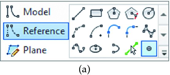
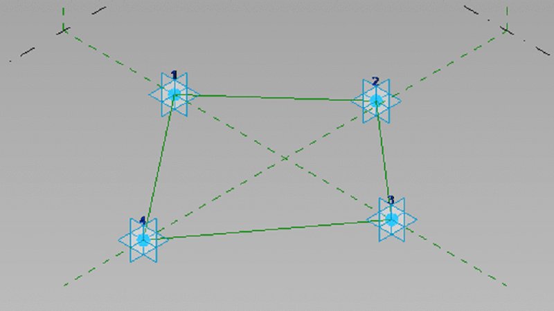
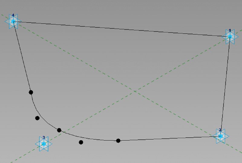
Switch to the Draw panel and select Reference and the Point Element tool. In the view window, create four points. These points aren’t location-specific; just lay them out relative to Figure 9.1. Lay the points out starting at the upper left and moving clockwise. These will later coincide with the number of vertical elements that you’ll create in the mass.
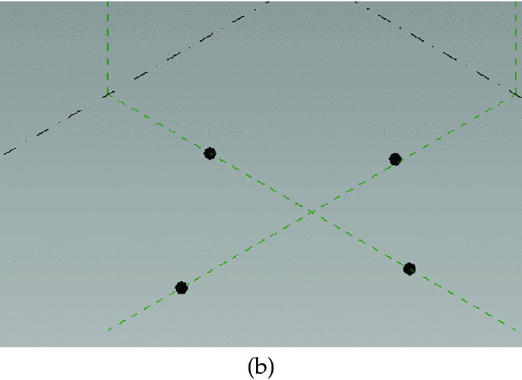
Click the Modify button, select all four points, and from the contextual tab in the ribbon, click the Make Adaptive tool.
The points will become numbered in the order in which they were inserted, and each point will have its own reference planes (Figure 9.2).
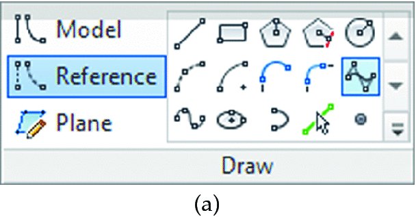
From the Create tab click Reference; then choose the Line command. Make sure that 3D Snapping is enabled from the Options bar. Starting with point 1, connect all four of the reference points to form an enclosed shape (Figure 9.3). Click the Modify button in the ribbon or press the Esc key twice to quit the Line command.
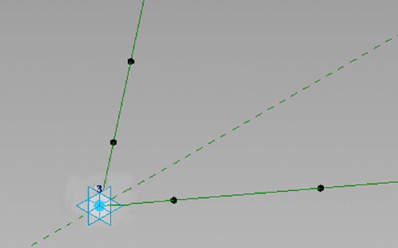
Now that you have all four points connected, forming a rhomboid, you will create a set of points to round one of the corners of the form. This rounded corner will be associated with a formula-based parameter so you can modify it within the mass to change its shape.
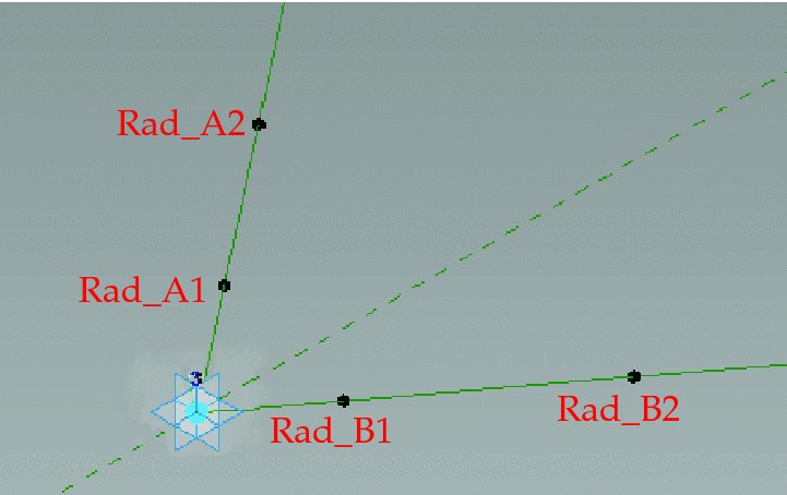
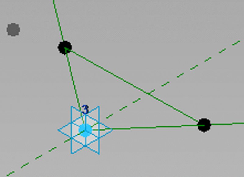
On the Create tab in the ribbon, click Reference, and choose the Point Element command. Make sure you choose the Draw On Face option to the right of the Draw tools. Add two points on the reference lines to each side of one of the corners. We’ve added points near corner 3, as illustrated in Figure 9.4.
For your next step, you need to add a parameter to control the location of the points along the reference line. The property of the point called Normalized Curve Parameter is a ratio of the length of the host line expressed from 0.0 to 1.0. If you want to keep a point at the midpoint of a reference line, this property must always be 0.5. If you select a point and you don’t see this property, you might need to delete the point and try placing it again; this ensures that you select the Draw On Face option in the Draw panel of the ribbon.
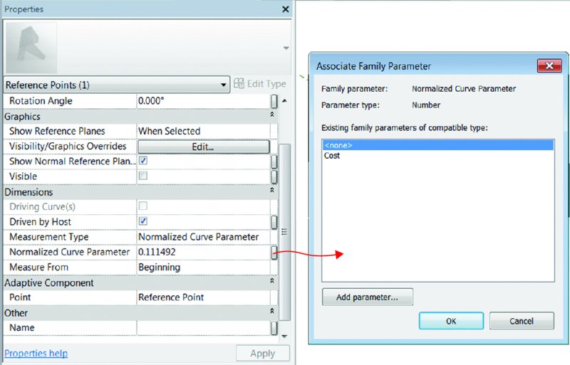
Start with the point closest to the corner between corners 3 and 4 (look ahead to Figure 9.7), and in the Properties palette locate the property named Normalized Curve Parameter. Click the small button to the right of the value field to pull up the Associate Family Parameter dialog box (Figure 9.5).
Click the Add Parameter button. This will open the Parameter Properties dialog box. Name the new parameter Rad_A1, and click OK to exit each of the dialog boxes. Choose the next point on that line and repeat this process, naming the point Rad_A2.
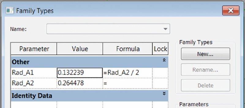
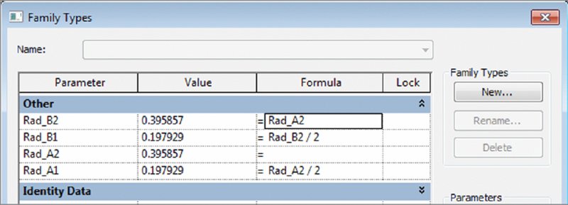
On the Create tab, click the Family Types tool. In the Family Types dialog box, you’ll see the two parameters you’ve created so far. You want to add a formula that will set point A1 at half the distance between points 3 and A2. In the Formula box for Rad_A1 add the formula =Rad_A2 / 2 (Figure 9.6). Click OK to exit the dialog box.
Repeat steps 6 and 7 with the points on the other line. For the other two points, select them as you did before and add the variables Rad_B1 and Rad_B2. The parameters should be associated with the points as shown in Figure 9.7.
Open the Family Types dialog box again and set Rad_B2 equal to Rad_A2. For Rad_B1 set the formula to read =Rad_B2 / 2. When you’ve finished, the Family Types dialog box should have four variables and three formulas, as shown in Figure 9.8. You can test the formulas by changing the numbers in the Value column and clicking Apply each time. You should see the points move up and down the host reference line.
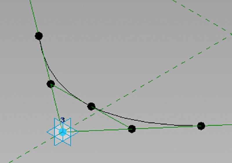
With these points and formulas in place, you’re going to add a few additional elements to create the curve. Add another reference line between the two middle points; be sure to select the 3D Snapping check box in the Options bar (Figure 9.9).
Switch to the Point Element command in the Draw panel, and then add a point to the middle of the reference line you added in the previous step.
In the Create tab, click Model and then select the Spline Through Points tool. Connect the farther point, Rad_A2, to the midpoint of the line to the point Rad_B2. The connected points should create an arc like the one shown in Figure 9.10.
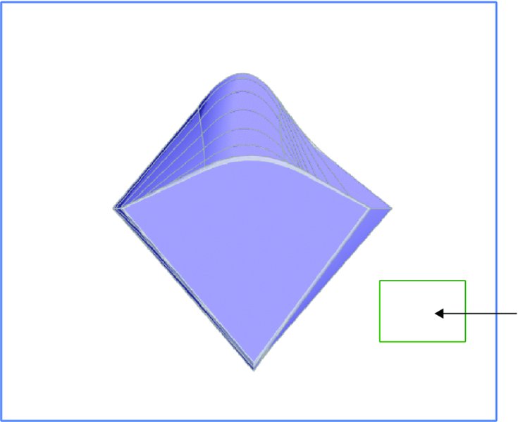
Make sure Model is still selected in the Create tab and choose the Line tool. Connect the arc you just created to the other three points, completing the shape. The final form will look like Figure 9.11 with the reference lines turned off.
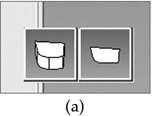
As the last step, you need to apply a surface. Select the model lines you just created either by using the Tab-select method or by selecting everything and then using the Filter tool to isolate Lines (Generic Model). From the contextual tab in the ribbon, choose Create Form ➢ Solid Form. You’ll be prompted with the option to create a solid or a plane. Choose the plane, which will be the option on the right (Figure 9.12). The result should look like the image to the right in the figure.
Figure 9.11 Adding model lines to connect the other points
Figure 9.12 Creating a form out of the model lines
At this point, you need to save the family for use in your mass. Save the family with the name c09-Adaptive-Rig.rfa. You can download the finished file from the Chapter 9 folder on this book’s web page, www.sybex.com/go/masteringrevitarch2016.
Building the Massing Framework
Now, you need to create a mass family into which you will load and place the adaptive component family. From the Application menu, choose New ➢ Conceptual Mass. This will open the template-selection dialog box. Choose the Mass.rft or Metric Mass.rft file. The conceptual mass environment will mirror the adaptive component look and feel. You’re going to use this to study forms for an office tower.
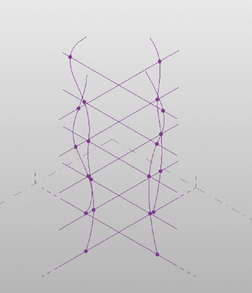
The first steps in this exercise will show you how to add some 3D splines, to which each of the four reference points in the adaptive component family will attach. With the new mass family started, follow these steps:
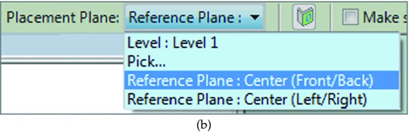
On the ViewCube® in the 3D view, click Front. In the Create tab of the ribbon, select Reference and choose the Spline tool. Before you place the point, set the Placement Plane drop-down on the Options bar to Reference Plane : Center (Front/Back), as shown in Figure 9.13.
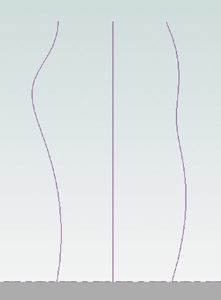
Draw one spline to the left and one to the right of the centerline (Figure 9.14). The shape of the spline isn’t important—keep it organic. To create a spline, you can click in the view as many times as you like, and then press the Esc key to stop sketching.
Orbit the 3D view slightly, and then click Left or Right from the ViewCube. Start the Reference + Spline tools again and choose Reference Plane : Center (Left/Right) from the Options bar. Draw two more reference splines, one on either side of the centerline.
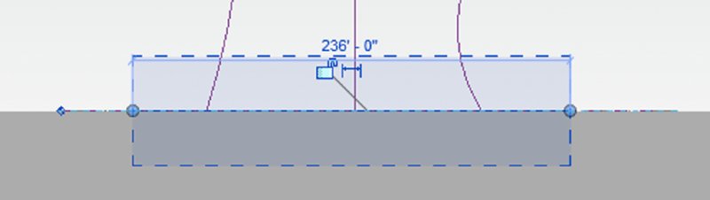
Your next step is to join the splines with horizontal reference lines. This will allow you to establish some benchmarks for inserting the platform family you just created. For each of the sets of horizontal reference lines you create, you’re going to insert another instance of the adaptive component family. To add the reference lines, you’ll draw those in the Left/Right plane to start. You want the reference lines to intersect both sets of points but to extend past them on both ends. The length of the reference line will determine how far the adaptive component can stretch. Start by drawing one at the base and extending it past both ends of the spline (Figure 9.15). Do the same for the Front/Back plane, making sure to remember to switch your placement plane.
Select one of the upper corners of the ViewCube so the view rotates back into an axonometric view. Next, you’re going to add points to the splines. Choose the Point Element tool and add a point to each of the splines near the intersections of the reference lines you just drew; see Figure 9.16. It doesn’t have to be exact—once you get all the points in place you’ll perform another step to connect the points to the intersection of the spline and reference line. Add four hosted points, one for each spline.
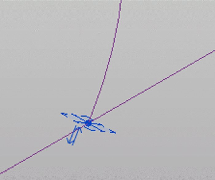
As we just mentioned, the next step is to attach the points to the reference lines. Select a point, and then choose Host Point By Intersection from the Options bar. Then choose the reference line, and the point will “jump” to the intersection of the spline and reference line, as shown in Figure 9.17. Do this for all four points.
Now, you need to make several versions of this—points with intersecting lines—one set for each of your adaptive components. Open one of your elevations (it doesn’t matter which one) by selecting one of the elevation sides of the ViewCube. Draw a selection box starting on the left and going right over the ground plane so you encompass the levels, points, and lines you’ve been drawing. You’ll have selected too much, but that’s okay. With everything selected, click the Filter tool in the contextual tab of the ribbon. In the Filter dialog box, uncheck Levels, Reference Points, and Reference Planes so that only Reference Lines is selected. Click OK to close the dialog box.
With these items selected, you’re going to make a few copies. In our example image (Figure 9.18) we’ve made three copies for a total of four elements. Choose the Copy tool from the Modify panel and copy these elements, spacing them relatively evenly. You’ll need to add points to each of these intersections. It’s a bit tedious, but it goes pretty quickly, and it will be good practice to remember the steps. Add the points on the splines and close the reference lines. Then select the points, choose Host By Intersection, and choose the reference line, as you did in step 6. When you’ve finished, you’ll have an array of points and lines, as shown in Figure 9.18.
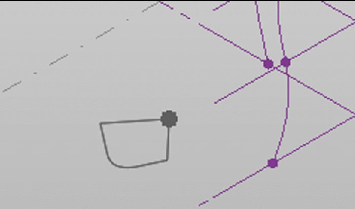
The mass is just about complete, and you’re ready to load the c09-Adaptive-Rig family into the project. Open the c09-Adaptive-Rig family file, or if the family is still open, choose the family from the Switch Windows button on the Quick Access toolbar. When you load an adaptive component into a family or project, it doesn’t respond quite like a normal component. The points you created need to be anchored to the points on the spline you created earlier. Load the platform family into the conceptual mass. Once it is loaded, one of the first things you’ll notice is a small, gray version of your family floating around by your cursor (Figure 9.19).
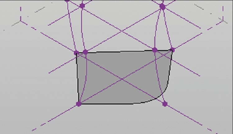
To anchor the family, select one of the points you inserted earlier in this chapter at the base of the splines. Work your way around all the points in the same plane in a clockwise fashion until you’ve selected all four points at the base of the spline (Figure 9.20). Notice how the curved section you added at point 3 isn’t touching the point on the vertical spline.
Do the same for each of the vertical levels you added. Your mass should look like Figure 9.21. Make sure your first point on each level is on the same spline. This will ensure that all the curved sections at point 3 stack properly. When your platforms are fully inserted, you can grab any of the splines and push and pull it to see the platforms change shape.
Before we create the solid form from these adaptive components, you will create a visibility toggle for the generic surfaces. This will allow you to turn them off in the project environment when you don’t need them.
Select each of the adaptive components you have placed in the 3D view. Click the Filter tool in the contextual tab of the ribbon and make sure that only Generic Models is selected. Click OK to close the Filter dialog box. In the Properties palette, click the Associate Family Parameter button for the property named Visible. Click Add Parameter in the dialog box.
In the Parameter Properties dialog box, set the Name of the new parameter as Show Rig and set the Group Parameter Under drop-down to Graphics. Click OK to close all open dialog boxes.
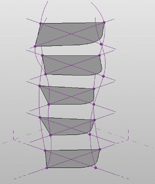
Finally, to create the mass, select the surface for each of the rigs. This is a somewhat tricky operation. You’ll need to hover the mouse pointer over the edge of a surface, press the Tab key slowly until you see Generic Models : c09-Adaptive-Rig : Face appear in the status bar at the bottom of the application window. Click to select the face. Then hover the mouse pointer over the next surface, and press the Tab key slowly as in the previous step. When you see the Face element in the status bar, press and hold the Ctrl key while clicking to select the next face. Repeat this process until all the faces are selected.
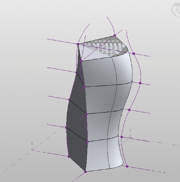
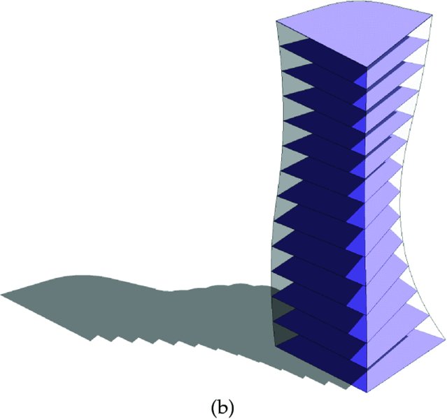
With these faces selected, select Create Form ➢ Solid Form from the contextual tab in the ribbon. Your completed mass will look like Figure 9.22. Remember to save the mass family for use in the next section of this chapter.
Figure 9.13 Select the correct work plane for the spline.
Figure 9.14 Draw two splines on either side of the work plane.
Figure 9.17 Aligning the points and reference lines
Figure 9.18 Creating several instances of the selection and adding points
Figure 9.19 Inserting the adaptive component into the mass
Figure 9.20 Anchoring the adaptive component to the mass
Figure 9.21 Creating several instances of the selection and adding points
Figure 9.22 Creating several instances of the selection and adding points
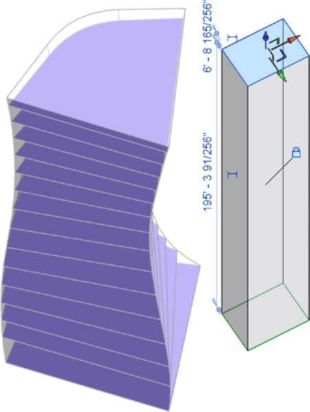
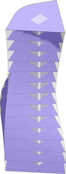
You can modify this mass by moving any of the nodes on the four vertical splines. You can also select any of the Adaptive Rig elements and click Edit Type in the Properties palette. Change the values for any of the Rad parameters you created in the adaptive component, and the severity of the curved edge will be affected. This exercise was just one example of the almost limitless number of ways you can use parameters and components to drive conceptual geometry. We’re going to use this mass family to explore conceptual energy analysis in the next section.
Energy Modeling
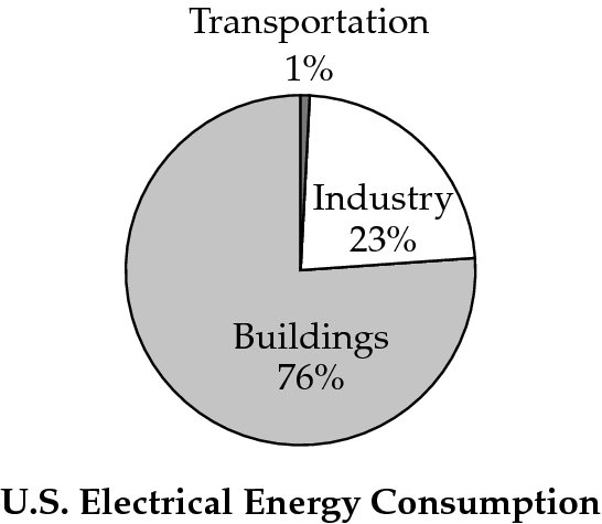
Understanding a building’s energy needs is paramount to helping the project become more sustainable. According to the U.S. Energy Information Administration (www.eia.doe.gov), as of March 2015 buildings in the United States account for 30 percent of the world’s energy consumption and 60 percent of the world’s electricity use, making the United States the primary consumer of energy in the world (Figure 9.23). This reality should inspire you to build responsibly and to think about your design choices before you implement them.
The energy needs of a building depend on a number of issues that are not simply related to leaving the lights on in a room that you are no longer using, turning down the heat, or increasing the air-conditioning. Many of the components and systems within a building affect its energy use. For instance, if you increase the size of the windows on the south façade, you allow in more natural light and lower your need for electric lighting. However, without proper sunshading, you are also letting in additional solar heat gain, so those larger windows are increasing your need for air-conditioning and potentially negating the energy savings from reduced lighting.
In exploring the use of energy in a building, you must consider all energy-related issues, which is a good reason to use energy-simulation tools. These computer-based models use climate data coupled with building loads, such as the following:
The heating, ventilation, and air-conditioning (HVAC) system
Solar heat gain
The number of occupants and their activity levels
Sunshading devices
Daylight dimming
Lighting levels
The energy model combines these factors to predict the building’s energy demands to help size the building’s HVAC system. It also combines the parameters of other components properly so you are not using a system larger than what you need, and you can understand the impact of your design on the environment. By keeping the energy model updated with the current design, you can begin to grasp how building massing, building envelopes, window locations, building orientation, and other parameters affect energy demands.
There are two ways you can use Revit Architecture software for energy analysis—by analyzing mass forms directly in the model or by exporting a more detailed model to another application using the gbXML format. The gbXML file type is a standardized XML schema that is used for sustainable design analysis. For either choice, you must first have accurate location and true north settings. Once you have those established, you can approach either analysis with confidence. Let’s first take a look at the process for generating a conceptual energy analysis.
Conceptual Energy Analysis
A conceptual energy analysis (CEA) tool was added to Revit software as a Subscription Advantage Pack in 2009. This tool creates a link to the online analysis service known as the Autodesk® Green Building Studio® service (www.autodesk.com/greenbuildingstudio). The analysis results will indicate such information as the life cycle and annual energy costs. In our opinion, it is wise to use the CEA tool only to determine which results are better or worse than others. If you convince your clients that these are the actual costs and they turn out to be too low when the building is constructed, will you be held responsible for the discrepancy?
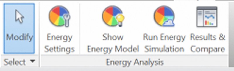
In the following exercise, you will load a conceptual mass into a template project to run a series of energy analyses. There are three basic tools for configuration, analysis, and comparison of results on the Analyze tab of the ribbon for both building elements and masses (Figure 9.24).
Figure 9.24 The Energy Analysis panel in the ribbon
Energy Analysis Setup
Before you can run an analysis for either building elements or massing, you need to do a bit of configuration to give your analysis engine some parameters to run. You’re going to use the mass you created, but you’re going to insert that mass into an existing building model so you can run the analysis side by side. Let’s get started by comparing the two buildings (existing and mass) side by side.
Open the c09-Analysis-Start.rvt or c09-Analysis-Start-Metric.rvt file. You can download the file from this book’s web page. Once the file is open, activate the Level 1 floor plan, and then load and insert the mass you made earlier in this chapter. You can also download the completed massing family from the web page (c09-Conceptual-Mass-Finished.rfa). Position the mass in the center of the plan view.
To begin the configuration of the energy analysis settings, follow these steps:
Activate the default 3D view, and in the view control bar, set Visual Style to Shaded and turn Shadows on. Select the massing form, and from the Properties palette click Edit Type. Deselect the Show Rig property and then click Apply. This will turn off the generic model faces from the adaptive component you used to build the massing form. Click OK to close the dialog box.
Activate the South elevation view. Use the Copy or Array tool to create several new levels that span the height of your massing family (Figure 9.25). Make the levels above Level 2 evenly spaced at 15′-0″ (4 m) each. Select the massing family again and from the contextual tab in the ribbon, click Mass Floors. Select all the levels in the dialog box and then click OK.
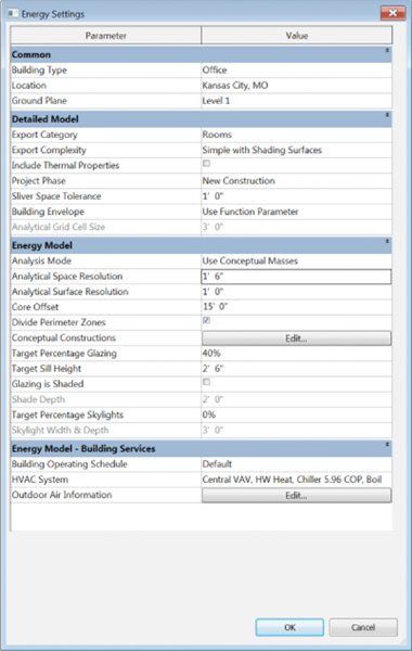
On the Analyze tab, click Energy Settings. The Energy Settings dialog box is shown in Figure 9.26. We’re going to work our way down this dialog box, making sure you have the settings correct. The first setting is Building Type. For the sake of our exercise, change this setting to Office.
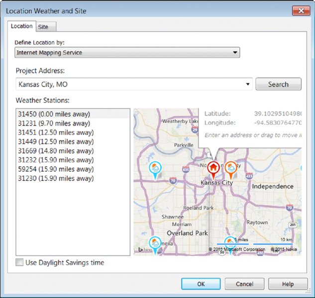
The next step is to establish the correct location of your project. Click the selection button to the right of the Location parameter to open the Location Weather And Site dialog box (Figure 9.27). Type Kansas City, MO, USA in the Project Address field and click Search. Click one of the closest weather stations (shown by the pin icons) in the list or directly on the map. You’re welcome to use your own location instead in this exercise. Finally, choose Use Daylight Savings Time if that is appropriate for your location and time of year. When you’ve made a selection, click OK to close the dialog box.
Set Ground Plane to Level 1.
You’ll notice a lot of options in the Energy Settings dialog box—some of them quite complex. To complete the rest of the dialog box, we’re going to step through each of the sections. So far, we’ve completed the first set of parameters in the Common group.
Let’s walk through the settings in the Detailed Model group:
Export Category Your option here is either Rooms or Spaces. If you’re working from an architectural model, chances are you’re using Rooms. If this were a MEP model or you were linking in information from an MEP consultant, you’d want to use Spaces. For our exercise, leave it set to Rooms.
Export Complexity There are five different levels of complexity that you can export your building model to. The least complex is a Simple model, and the complexity grows to include shading, surfaces, and mullions. To use the more complex features, you’ll need to have that content available in the model, and it will take more time to render a result. Leave the default setting of Simple With Shading Surfaces.
Include Thermal Properties This check box will include the thermal properties of materials you have in your building design. In the Materials dialog box, you have the ability to add thermal values (R and U values) to the materials used for modeled elements such as walls, windows, and roofs. For this exercise, we are analyzing only conceptual massing, so deselect the check box.
Project Phase This is the phase the analysis will be run against. Keep the default setting of New Construction.
Sliver Space Tolerance This setting specifies the gap between spaces or rooms that is acceptable for the analysis. Leave the default setting of 1′-0″ (300 mm).
Building Envelope This setting is used only for analyzing building elements—not conceptual massing. The options are to use the Function parameter of walls to determine if it is set to Exterior or to identify the walls dynamically using ray-trace and flood-mapping calculation methods.
Analytical Grid Cell Size Used with the Building Envelope setting, this dimension sets the specificity of the calculation method to determine the exterior walls. The smaller the value, the longer the calculation will take.
The next group of settings comprises the Energy Model parameters. These settings deal with more complex energy model parameters and usually require some input from your mechanical consultant. We’ll explain the parameters here, but for this section plan to keep the default values of our exercise.
Analysis Mode This setting allows you to decide what type of elements you wish to use for your analysis. There are three options: Use Building Elements, Use Conceptual Masses, and Use Conceptual Masses And Building Elements. Depending on the phase of your design, you’ll need to decide which of these configurations to use. For our massing analysis, choose Use Conceptual Masses.
Analytical Space Resolution and Analytical Surface Resolution These numbers dictate the tolerances for Revit to resolve the spaces and surfaces within the model. For our uses, keep the default values.
Core Offset This is the distance the building core is offset from the perimeter. If you have an assumption for this distance in the early design phases of your project, you can define it here. For this example, use 15′ (4.5 m).
Divide Perimeter Zones When this setting is enabled (the default), zones are automatically defined around the perimeter of the massing form. If you prefer to create your own zones, disable this setting and set the Core Offset value to 0. Then create more detailed mass forms and use the Cut Geometry tool to combine overlapping forms.
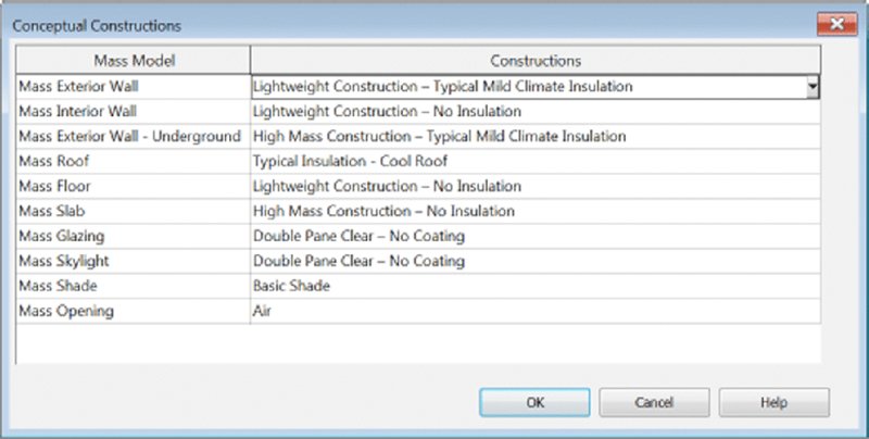
Conceptual Constructions The Conceptual Constructions button allows you to edit the assumed values of building elements for the mass form, as shown in Figure 9.28.
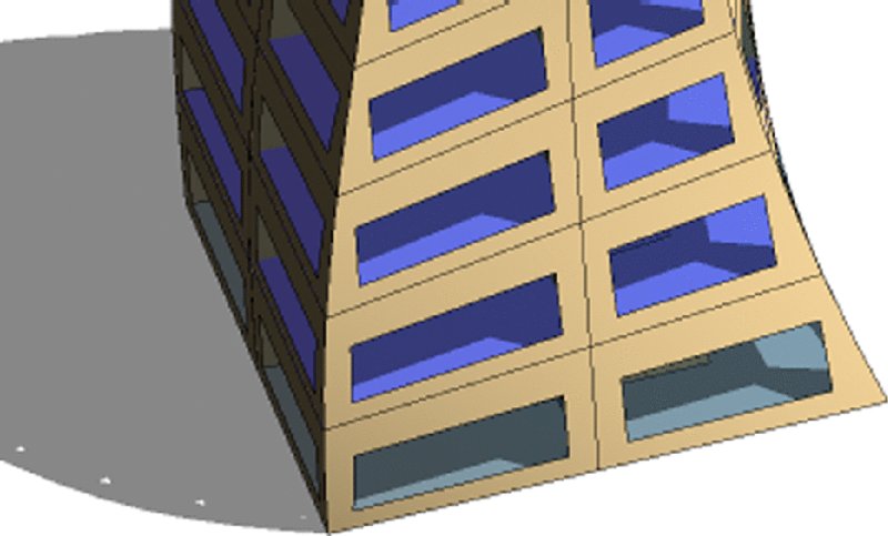
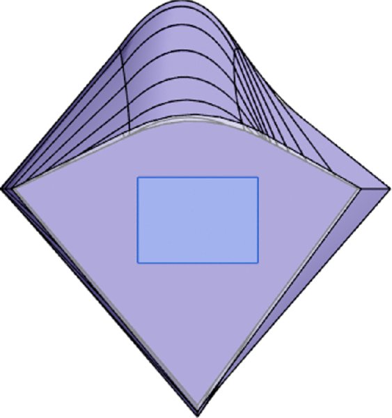
Target Percentage Glazing When you click the Show Energy Model button, you will see the Target Percentage Glazing value illustrated as solid and semi-transparent regions on the vertical exterior surfaces of the massing form (Figure 9.29). This value sets the assumed amount of glazing as a percentage of the overall wall area.
Target Sill Height This is the height of the sill for glazing to begin on each floor.
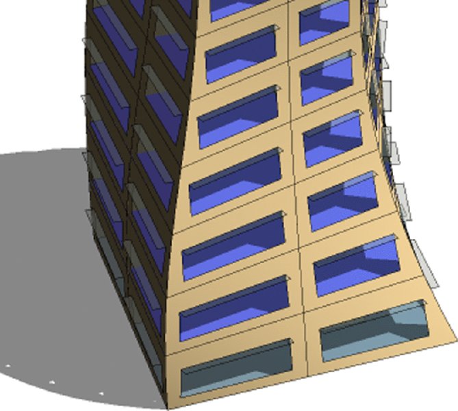
Glazing Is Shaded Select this check box if you intend to design sunshading for the glazing. This does not differentiate by building orientation, so if you check the box, conceptual shading elements will be added to the glazing assumptions on all sides (Figure 9.30).
Shade Depth When the Glazing Is Shaded option is checked, you can assign a depth to any assumed sunshading.
Target Percentage Skylights Like Target Percent Glazing, this value assumes an amount of skylighting for your model.
Skylight Width & Depth This value sets the size for skylights if you are using that value.
The last grouping in this dialog box is Energy Model – Building Services. Like the previous set of values, these require a bit of advanced knowledge of the building operation cycle and some assumptions about your HVAC system. For our example, leave the default values.
Building Operation Schedule How often will your building be occupied? Will it have people in it 24/7, or will it be operational only during office hours? This can have a large impact on your heating and cooling cycles.
HVAC System Here you can set a conceptual HVAC system. That could be a four-pipe system, underfloor air distribution, or a variety of other HVAC system types.
Outdoor Air Information If you know how many air exchanges you’ll be required to produce per hour, you can set that value here.
Once those values are set, click OK to exit the dialog box.
Remember that this type of analysis is based on assumptions only and uses the overall size, location, and orientation of your proposed design. After you start analyzing the results, you can examine different massing configurations with the same construction and systems assumptions or varied assumptions on the same massing configuration.
Figure 9.27 In Location Weather and Site, first specify the location and weather station.
Figure 9.28 Conceptual Constructions allow you to test assumptions about massing forms.
Figure 9.29 Assumptions for glazing are illustrated on exterior surfaces of the massing form at the default of 40%.
Figure 9.30 Conceptual shading elements are added to all sides of the massing form.
Running Energy Analysis Simulations
After you have established some baseline settings and assumptions for an energy analysis, it’s time to begin running simulations. These types of simulation are run from 3D views, so you might notice that the Run Energy Simulation button is grayed out if you are working in a 2D view such as a plan or elevation. This view-specific behavior also gives you the ability to create design options for your massing studies, for which you will be able to compare the results. We cover design options in Chapter 10, “Working with Phasing, Groups, and Design Options.”
Let’s continue the conceptual energy analysis exercise by running some simulations. Follow these steps:
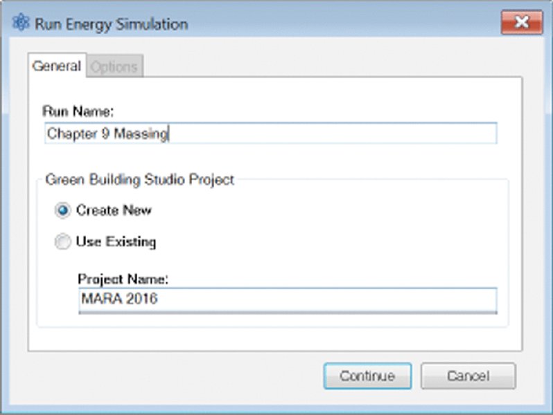
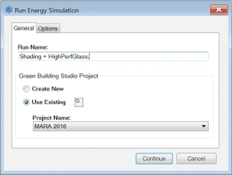
Click the Run Energy Simulation button on the ribbon to start the analysis. If you haven’t logged into A360, you’ll be asked to sign in. Next, you’ll get a dialog box asking you to name your new simulation. We’ve filled this in with some project-specific values, but you can name this whatever you’d like (Figure 9.31). You will need an Internet connection and an Autodesk Subscription account to run energy simulations. Once you click Continue, Revit will begin uploading your energy data.
In the Run Energy Simulation dialog box, name this analysis Baseline_SouthCurve and click to run your initial analysis. The software will start to communicate with the Green Building Studio service. Click Continue. This will take a few minutes to run. Your model data will be sent off to their cloud for processing and allow you to continue working while the analysis is being performed.
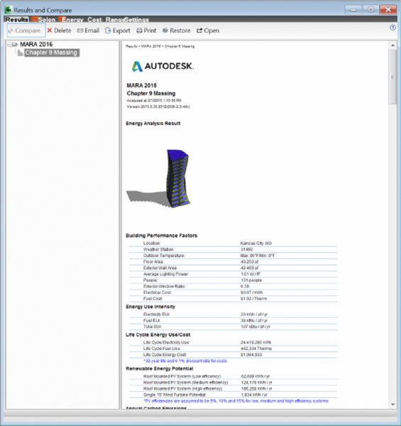
Click the Results & Compare button on the ribbon to view the progress of the upload. If you don’t have the Results And Compare dialog box open, an alert will appear in the lower-right portion of the application window, informing you that the analysis is complete. Once it is complete, you will see the run listed under the name of the model you are analyzing, as shown in Figure 9.32. You can scroll through the list of analyses that are provided.
You can scroll through the results and get a basic understanding of the building loads (Figure 9.33). One of the great uses for this tool isn’t looking at the actual reported data but using it as a comparative analysis. If you make changes to the building form, size, or orientation, how does that change your performance?
Activate the plan view named Site from the Project Browser. Select the massing family and select the Rotate tool from the contextual tab in the ribbon. Rotate the mass so that the curved face is oriented South (90 degrees counterclockwise).
Return to the default 3D view and switch to the Analyze tab in the ribbon. Click the Run Energy Simulation button, and then enter a new name in the Run Name field. Select the Use Existing radio button, and choose your project name from the drop-down list, as shown in Figure 9.34.
Now let’s make some adjustments to the building’s energy settings (not the mass) and rerun the results:
Go back to the main application window and click the Energy Settings button on the ribbon. Select the Glazing Is Shaded check box and set the Shade Depth value to 2′-0″ (600 mm).
Click the Conceptual Constructions Edit button and change the Mass Glazing setting to Double Pane Clear - High Performance, LowE, High Tvis, Low SHGC. Click OK to close both dialog boxes.
Click the Run Energy Simulation button again, name this run Shading + HighPerfGlass, and choose to use the existing model.
After the run has completed, return to the Results And Compare window, press and hold the Ctrl key, and select both the Baseline_SouthCurve and Shading + HighPerfGlass runs. Click the Compare button.
Figure 9.31 Generate the analytical energy model to begin the simulation.
Figure 9.34 Create another simulation run for the existing project.
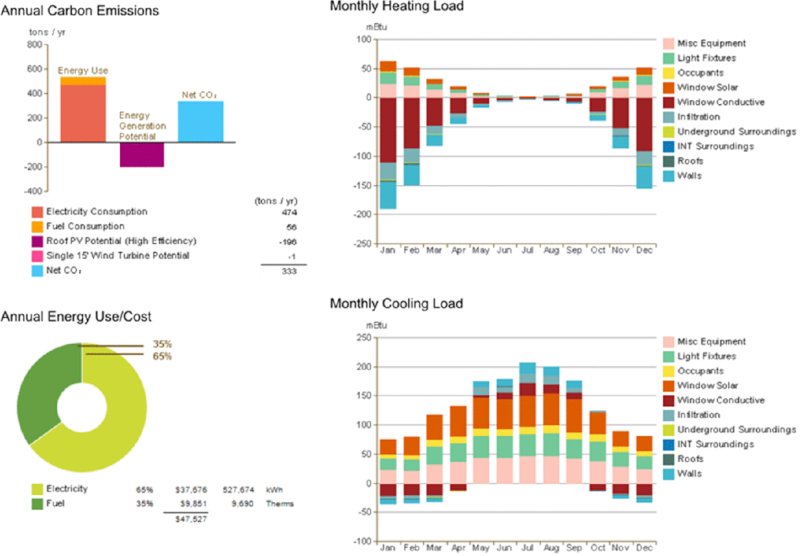
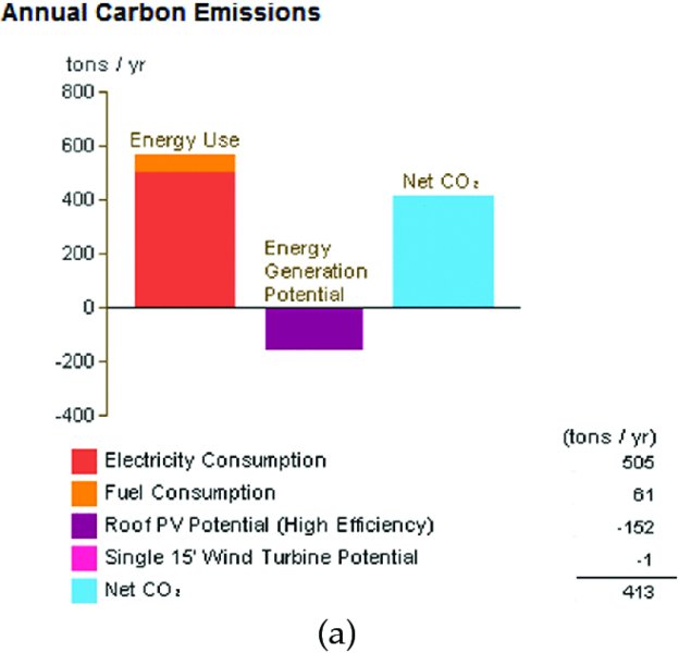
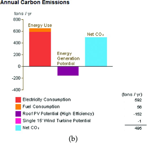
You will see the results of the two analyses runs side by side. Notice that the second run has a lower monthly electricity consumption and lower fuel consumption. Be careful when reading the graphs, because the values in each graph may be different. Take a look at the Monthly Cooling Load graphs. Notice that the values for Window Solar are lower for the second run; however, the values for Light Fixtures are slightly higher. This is due to the addition of the shading, which requires more electric lighting power.
Refining the Conceptual Analysis
In these initial analysis runs, we used and edited the default settings; however, these settings are applied to the whole building form. What if you want to refine your studies to examine more specific design assumptions? In the following exercise, you will continue to examine the conceptual tower mass, but you will select and modify individual faces of the geometry so they no longer follow the overall assumptions established in the Energy Settings dialog box.
Continue with the c09-Analysis-Start or c09-Analysis-Metric project, and follow these steps:
Activate the default 3D view and orbit the view so the two flat vertical faces of the mass family are shown in the view.
Because there are so many intricate parts to a massing form that has been enabled as an energy model, there are a few tricks to selecting the most appropriate objects. Follow the next steps carefully or you may be confused by settings and properties that appear differently than those illustrated here.
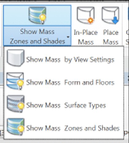
In the Select flyout menu below the Modify button, make sure that Select Elements By Face is checked. On the Massing & Site tab, set the Show Mass Surface Types flyout button to Show Mass Surface Types, as shown in Figure 9.35.
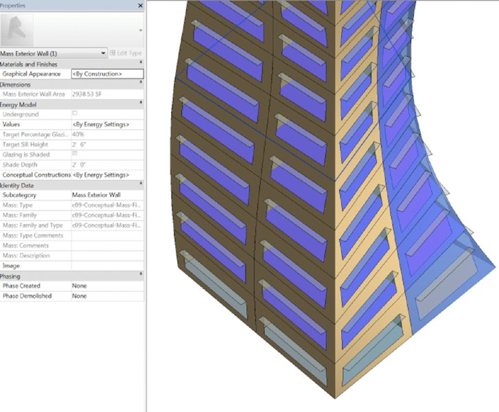
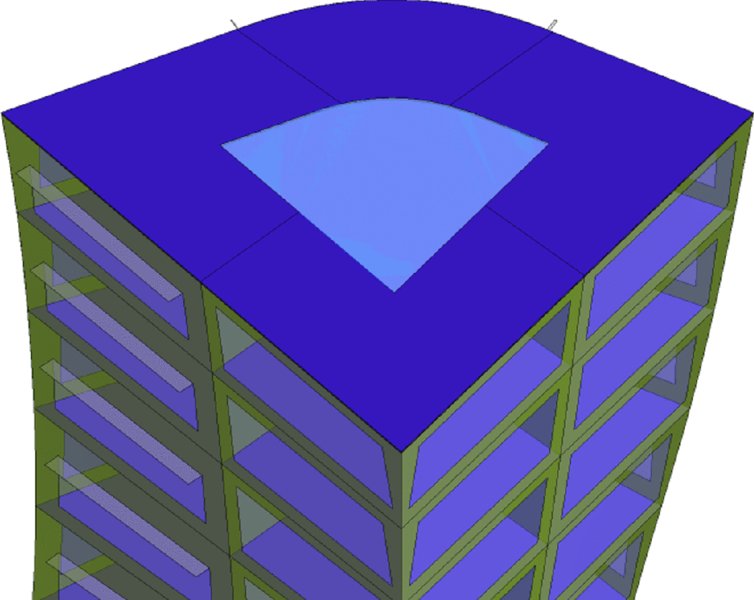
Hover the mouse cursor over an opaque part of the exterior surface of the mass form. Press the Tab key slowly until you see the element in the status bar that ends with “Shape Handle” and then click to select it. The surface you should be selecting is the Mass Exterior Wall, as indicated in the Properties palette (Figure 9.36).
In the Properties palette, under the Energy Model settings, set the Values property to <By Surface>. Then set the following values:
Target Percentage Glazing: 60%
Glazing Is Shaded: Unchecked
Repeat steps 3 and 4 for all the Mass Exterior Wall surfaces on the two flat sides of the massing form.
Because these surfaces are oriented toward the north, we may be able to avoid the cost of the sunshades and increase the glazing area to allow more natural light into the interior spaces for a possible reduction in artificial lighting costs without increasing solar heat gain.
From the Analyze tab, click Run Energy Simulation. Set the Run Name to North Faces Refined, and be sure to select the Use Existing radio button and choose your existing project from the drop-down list.
When the simulation is complete, click the Results & Compare button in the Analyze tab of the ribbon. In the Results And Compare dialog box, select both the North Faces Refined and Shading + HighPerfGlass runs, and then click Compare.
Figure 9.36 Select an individual surface of the conceptual massing energy model.
Examining the results in these two examples may reveal some interesting comparisons. It seems that the overall energy use intensity (EUI) and carbon emission are estimated to be higher with the refined model than the previous run that included sun shading and high-performance glazing on the entire exterior enclosure (Figure 9.37). By increasing the percentage of glazing on the northern faces, we may be increasing the amount of natural light, but we are also increasing the surface area of a less-efficient enclosure material. As a result, the winter heating load increases.
Figure 9.37 Comparing carbon emissions between two simulation runs
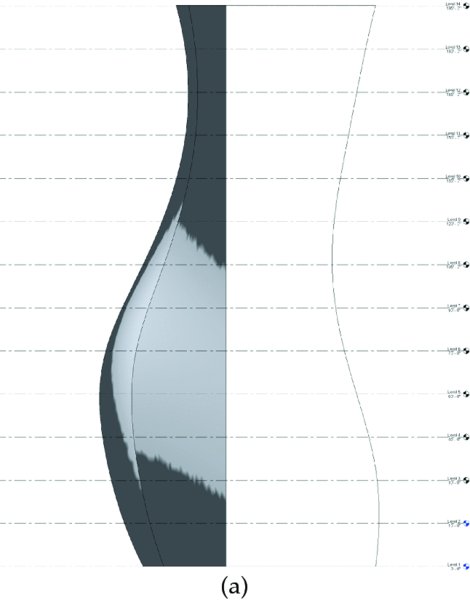
As a final exercise to examine methods for refining your conceptual analysis model, we will add an extruded in-place mass that will represent a slightly more accurate depiction of a building core. As we mentioned earlier in this chapter, the Divide Perimeter Zones option in the Energy Settings dialog box is checked by default. This setting creates a simulated zone that is offset from the exterior face of the massing form (Figure 9.38). If the exterior faces of the massing form are irregularly shaped, the simulated core will be irregularly shaped as well.
Let’s create a slightly more accurate representation of our building core with a quick exercise. We will continue to use the c09-Analysis-Start or c09-Analysis-Start-Metric file. To get started, follow these steps:
From the Analyze tab in the ribbon, click to deselect the Show Energy Model setting. You should see the massing form as you did at the beginning of the exercises in this chapter.
Switch to the Massing & Site tab and click In-Place Mass. Name the new mass Building Core and then click OK to continue.
Orient the default 3D view to a plan view. You can do this by clicking Top on the ViewCube. In the Create tab of the ribbon, choose Reference, the Rectangle drawing tool, and the Draw On Work Plane setting. Make sure that Level 1 is specified as the Placement Plane in the Options bar.
Draw a rectangle next to the tower massing form, as shown in Figure 9.39. The exact size is not important for the purpose of this exercise. We just want it to fit completely inside the tower massing form after we extrude the shape.
Orbit the 3D view back to an orthogonal projection. Click the Modify button in the ribbon (or press the Esc key), and select the rectangular sketch. From the contextual tab in the ribbon, select Create Form ➢ Solid Form and then choose the In Context option to generate a solid extrusion.
Select the top surface of the extrusion and use the shape arrow to drag the extrusion to be as tall as the tower massing form, as shown in Figure 9.40.
Click Finish Mass in the ribbon, and then select the mass you just created. Click the Mass Floors tool in the ribbon, and select all the levels in the Mass Floors dialog box.
In the 3D view, click Top on the ViewCube. Select the extruded building core mass and move it within the tower massing form, as shown in Figure 9.41.
On the Modify tab in the ribbon, click the Join Geometry (or Join) tool. First, choose the core massing form, and then choose the tower massing form. The order of picking is important. If you pick the tower first and then the core, the core mass will disappear.
Orbit the 3D view and you should see the extruded form extending the entire height of the tower form, as shown in Figure 9.42.
In the Analyze tab in the ribbon, click Energy Settings. Uncheck the Divide Perimeter Zones option and set the Core Offset value to 0 (zero). Click OK to close this dialog box, and then click Show Energy Model. You will see that the perimeter zones are now defined by the core mass extrusion instead of a default offset from the exterior face of the tower massing form (Figure 9.43).
Figure 9.39 Sketch a rectangular shape outside the massing form.
Figure 9.40 Make the extrusion as tall as the tower form.
Figure 9.41 Move the core mass into the tower form.
Figure 9.42 The core mass is now joined with the tower mass.
Figure 9.43 The energy model is enabled with the massing core.
You can now run additional simulations and compare the results to those from our earlier exercises. Subtle differences may be identified in terms of the amount of heating and cooling because of a more accurate representation of the perimeter spaces.
As you can see, generating a sustainable design for your projects is a process of testing a variety of options and comparing the results. We have shown you a simple example to make you familiar with the basic process. It is up to you to explore these options further in the context of your own designs.
Detailed Energy Modeling
Later in the design process, you may want to use your building elements to perform more detailed energy modeling. For this process to be successful, you first need a solid, well-built model. This does not mean you need to have all the materials and details figured out, but you do have to establish some basic conditions. To ensure that your model is correctly constructed to work with an energy-modeling application, there are a few things you need to do within the model to get the proper results. Some of this might sound like common sense, but it is important to ensure that you have the following elements properly modeled or you may have incorrect results:
The model must have roofs and floors.
Walls inside and outside need to touch the roofs and floors.
All areas within the analysis should be bound by building geometry (no unbound building geometry allowed).
To perform an energy analysis, you need to take portions of the model and export them using gbXML to an energy-analysis application. The following are the energy-modeling applications commonly used within the design industry. They vary in price, ease of use, and interoperability with a gbXML model. Choosing the correct application for your office or workflow will depend on a balance of those variables.
IES VE IES VE (www.iesve.com) is a robust energy-analysis tool that offers a high degree of accuracy and interoperability with a design model. The application can run the whole gamut of building environmental analysis, from energy and daylighting to computational fluid dynamics (CFDs) used to study airflow for mechanical systems. Cons to this application are its current complexity for the user and the relatively expensive cost of the tool suite.
Autodesk® Ecotect® Analysis Software This application (www.autodesk.com/ecotect-analysis) has a great graphical interface and is easy to use and operate. The creators of this application also have a number of other tools, including a daylighting and weather tool. Although the program is easy to use, it can be challenging to import model geometry depending on what application you are using for your design model. For example, SketchUp and Vectorworks can import directly, whereas applications like Revit can be more of a challenge.
eQuest The name stands for the Quick Energy Simulation Tool (www.doe2.com/equest). This application is a free tool created by the Lawrence Berkeley National Laboratory (LBNL). It’s robust and contains a series of wizards to help you define your energy parameters for a building. As with Ecotect, it can be a challenge to import a design model smoothly depending on the complexity of the design, although it will directly import SketchUp models by using a free plug-in.
Exporting to gbXML
Before you can export the model to gbXML and run your energy analysis, you need to create several settings so you can export the proper information. The order in which these options are set isn’t important, but it is important to check that they are set before exporting to gbXML. If the information within the model is not properly created, the results of the energy analysis will be incorrect.
PROJECT LOCATION
As we mentioned earlier in this chapter, the physical location of the project on the globe is an important factor in energy use analysis. You can give your building a location in a couple of ways. One is to choose the Manage tab and click the Location button. Another way to get to this same dialog box is through the Graphic Display Options dialog box you used for sunshading earlier in this chapter.
BUILDING ENVELOPE
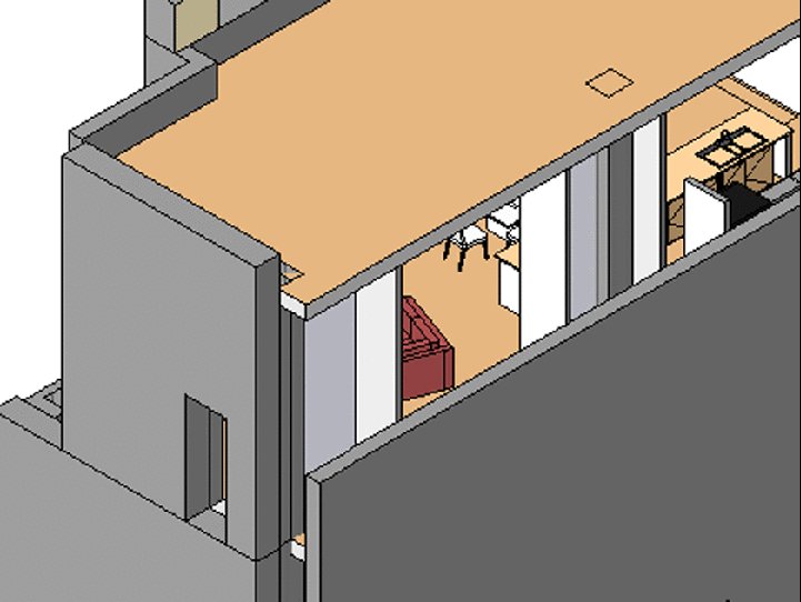
Although this might seem obvious in concept, you cannot run an accurate energy analysis on a building without walls. Although the specific wall or roof composition won’t be taken into account, each room needs to be bound by a wall, floor, or roof. These elements are critical in creating the gbXML file and defining the spaces or rooms within the building. These spaces can in turn be defined as different activity zones in the energy-analysis application. Before you export, verify that you have a building envelope free of unwanted openings. This means all your walls meet floors and roofs and there are no “holes” in the building (Figure 9.44).
Figure 9.44 Make sure your building envelope is fully enclosed.
ROOMS AND VOLUMES
When you export to a gbXML file, you are actually exporting the room volumes because they are constrained by the building geometry. This is what will define the zones within the energy-analysis application. You will need to verify several things to make sure your rooms and room volumes are properly configured:
Ensure that all spaces have a room element. Each area within the model that will be affected by the mechanical system will need to have a room element added to it. To add rooms, select the Room tool from the Architecture tab.
Set room heights. Once all the rooms are placed, each room’s properties should be redefined to reflect its height. The height of the room should extend to the bottom of the room above (in a multistory building), or if it is the top floor or only floor of a building, the room must fully extend through the roof plane. When you extend the room through the roof plane, the software will use the Roof geometry to limit the height of the room element and conform it to the bottom of the roof. Rooms should never overlap either in plan (horizontally) or vertically (between floors) because this will give you inaccurate results.
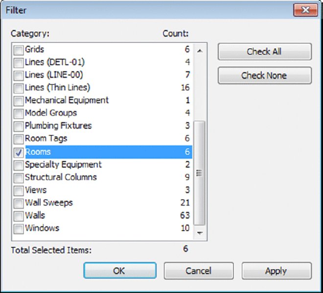
An easy way to set the room heights is to open each level and select everything. Using the Filter tool (Figure 9.45), you can deselect all the elements and choose to keep only the rooms selected. In this way, you can edit all the rooms on a given floor at one time.
Figure 9.45 Use the Filter tool to select only the rooms.
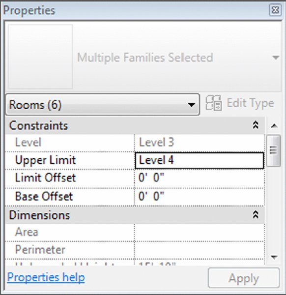
Once the rooms are selected, go to the Properties palette and modify the room heights. By default, rooms are inserted at 8′-0″ high, and the default for metric projects is 4 m. You have the option to set a room height directly, or you can modify the room height settings to go to the bottom of the floor above. This second option is shown in Figure 9.46. Note that you’ll need to set Upper Limit to the floor above and set the Limit Offset value to 0 (zero). Repeat this same workflow for every floor of the building.
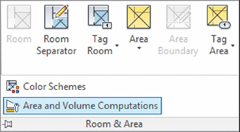
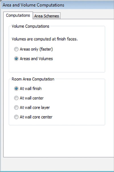
Turn on room volumes. Now that all the heights are defined, you have to tell the application to calculate the volumes of the spaces. By default, Revit does not perform this calculation. Depending on the size of your file, leaving this setting on can hinder performance. Make sure that after you export to gbXML, you return to the Area And Volume Computations dialog box from the Room & Area panel on the Architecture tab and change the setting back to Areas Only.
To turn on room volumes, select the flyout menu from the Room & Area panel on the Architecture tab (Figure 9.47) and click Area And Volume Computations.
Doing so opens the Area And Volume Computations dialog box. There are a couple of simple settings here that will allow you to activate the volume calculations (Figure 9.48). You’ll want to select the Areas And Volumes radio button on the Computations tab so that the software will calculate in the vertical dimension as well as the horizontal for your room elements.
Figure 9.48 Enabling volume calculations for rooms
The Room Area Computation setting tells Revit from where in the wall to calculate rooms. If you choose At Wall Finish, the software will not calculate any of the space a wall actually takes up with the model. Arguably, this is also conditioned space. Technically, what you would want is to calculate from the wall centers on interior partitions and the interior face of walls on exterior walls. However, you do not have that option, so choose to calculate from At Wall Center. Once you’ve modified those settings, click OK.
EXPORTING TO gbXML
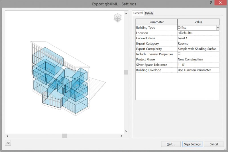
Now that you have all the room settings in place, you’re ready to export to gbXML. To start this process, click the Application menu and select Export ➢ gbXML. If this step opens the Space Volumes Not Computed warning, be sure to select Yes. This will enable Revit to calculate volumes instead of just areas. Once you do that, a dialog box like the one in Figure 9.49 will open, allowing you to refine your settings for a gbXML export.
There are a few things to take note of in this dialog box. First, you’ll see a 3D image of the building showing all the room volumes that are bound by the exterior building geometry. You can see in our building visualization that the boundary for the building is not completely full of room elements and that some of the room elements do not visually extend to the floor above. This would be your first clue that all your rooms do not have room elements placed or set properly, and you’ll want to dismiss this dialog box to change those settings.
Second, you’ll notice the ViewCube feature at the upper right of the 3D view window. This window will respond to all the same commands that a default 3D view will, directly in the Revit interface, allowing you to turn, pan, and zoom the visualization.
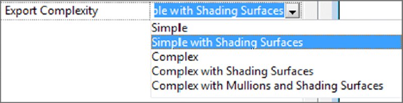
There are also two tabs on the right of this dialog box. The General tab contains general information about your building (building type, location, ground plane, and project phase), and you’ll want to verify that it is filled out properly. These settings will help determine the building use type (for conceptual-level energy modeling) and the location of your building in the world. There are two other settings that you’ll need to be aware of: Sliver Space Tolerance and Export Complexity. Sliver Space Tolerance will help take into account that you might not have fully buttoned up your Revit building geometry. This will allow you a gap of up to a foot, and the software will assume that those gaps (12″/300 mm or less) are not meant to be there. The Export Complexity setting allows you to modify the complexity of the gbXML export. You have several choices (Figure 9.50) based on the complexity of your model and the export. These are identical to the ones found in the Energy Settings dialog box.
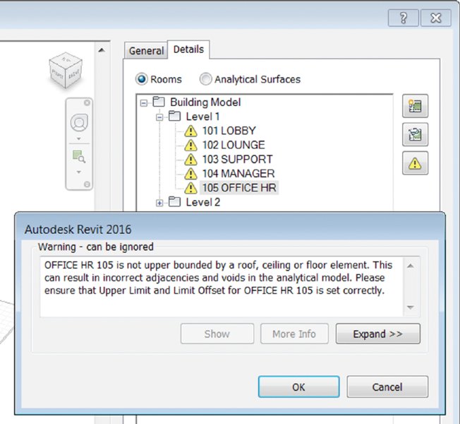
The Details tab will give you a room-by-room breakdown of all the room elements that will be exported in the gbXML model. Figure 9.51 shows the expanded Details tab. This is an important place to check because, as you’ll also notice, this dialog box will report errors or warnings with those room elements.
Figure 9.51 The Details tab allows you to examine any errors or warnings.
If you expand any of the levels and select a room, clicking the warning triangle will give you a list of the errors and warnings associated with that room. You’ll want to make sure your gbXML export is free of any errors or warnings before completing the export.
Once you’re ready to finish the export, click Next. This will give you the standard Save As dialog box, allowing you to locate and name your gbXML file. Depending on the size and complexity of your building, a gbXML export can take several minutes and the resulting file size can be tens of megabytes.
You’re now ready to import the gbXML file into your energy analysis application to begin computing your energy loads.
The Bottom Line
Embrace energy analysis concepts. Understanding the concepts behind sustainable design is an important part of being able to perform analysis within the Revit model and a critical factor in today’s design environment.
Master It What are four key methods for a holistic sustainable design?
Create a conceptual mass. Understand ways to generate building forms quickly and easily to explore a variety of shapes and orientations.
Master It Describe how you can use families to quickly generate form.
Analyze your model for energy performance. Being able to predict a building’s energy performance is a necessary part of designing sustainably. Although Revit doesn’t have an energy-modeling application built into it, it does have interoperability with many applications that have that functionality.
Master It Explain the steps you need to take to get a Revit model ready for energy analysis.