Chapter 20: Profiling and Tracing

Interactive debugging using a source-level debugger, as described in the previous chapter, can give you an insight into the way a program works, but it constrains your view to a small body of code. In this chapter, we will look at the larger picture to see whether the system is performing as intended.

Programmers and system designers are notoriously bad at guessing where bottlenecks are. So if your system has performance issues, it is wise to start by looking at the full system and then work down, using more sophisticated tools as you go. In this chapter, I'll begin with the well-known top command as a means of getting an overview. Often the problem can be localized to a single program, which you can analyze using the Linux profiler, perf. If the problem is not so localized and you want to get a broader picture, perf can do that as well. To diagnose problems associated with the kernel, I will describe some trace tools, Ftrace, LTTng, and BPF, as a means of gathering detailed information.

I will also cover Valgrind, which, because of its sandboxed execution environment, can monitor a program and report on code as it runs. I will complete the chapter with a description of a simple trace tool, strace, which reveals the execution of a program by tracing the system calls it makes.

In this chapter, we will cover the following topics:

• The observer effect
• Beginning to profile
• Profiling with top
• The poor man's profiler
• Introducing perf
• Tracing events
• Introducing Ftrace
• Using LTTng
• Using BPF
• Using Valgrind
• Using strace

Technical requirements

To follow along with the examples, make sure you have the following:

• A Linux-based host system
• Buildroot 2020.02.9 LTS release
• Etcher for Linux
• A Micro SD card reader and card
• A Raspberry Pi 4
• A 5 V 3A USB-C power supply
• An Ethernet cable and port for network connectivity

You should have already installed the 2020.02.9 LTS release of Buildroot for Chapter 6, Selecting a Build System. If you have not, then refer to the System requirements section of The Buildroot user manual (https://buildroot.org/downloads/manual/manual.html) before installing Buildroot on your Linux host according to the instructions from Chapter 6.

All of the code for this chapter can be found in the Chapter20 folder from the book's GitHub repository: https://github.com/PacktPublishing/Mastering-Embedded-Linux-Programming-Third-Edition.

The observer effect

Before diving into the tools, let's talk about what the tools will show you. As is the case in many fields, measuring a certain property affects the observation itself. Measuring the electric current in a power supply line requires measuring the voltage drop over a small resistor. However, the resistor itself affects the current. The same is true for profiling: every system observation has a cost in CPU cycles, and that resource is no longer spent on the application. Measurement tools also mess up caching behavior, eat memory space, and write to disk, which all make it worse. There is no measurement without overhead.

I've often heard engineers say that the results of a profiling job were totally misleading. That is usually because they were performing the measurements on something not approaching a real situation. Always try to measure on the target, using release builds of the software, with a valid dataset, using as few extra services as possible.

A release build usually implies building fully optimized binaries without debug symbols. These production requirements severely limit the functionality of most profiling tools.

Symbol tables and compile flags

Once our system is up and running, we will hit a problem right away. While it is important to observe the system in its natural state, the tools often need additional information to make sense of the events.

Some tools require special kernel options. For the tools we are examining in this chapter, this applies to perf, Ftrace, LTTng, and BPF. Therefore, you will probably have to build and deploy a new kernel for these tests.

Debug symbols are very helpful in translating raw program addresses into function names and lines of code. Deploying executables with debug symbols does not change the execution of the code, but it does require that you have copies of the binaries and the kernel compiled with debug information, at least for the components you want to profile. Some tools work best if you have these installed on the target system: perf, for example. The techniques are the same as for general debugging as I discussed in Chapter 19, Debugging with GDB.

If you want a tool to generate call graphs, you may have to compile with stack frames enabled. If you want the tool to attribute addresses with lines of code accurately, you may need to compile with lower levels of optimization.

Finally, some tools require instrumentation to be inserted into the program to capture samples, so you will have to recompile those components. This applies to Ftrace and LTTng for the kernel.

Be aware that the more you change the system you are observing, the harder it is to relate the measurements you make to the production system.

Tip

It is best to adopt a wait-and-see approach, making changes only when the need is clear, and being mindful that each time you do so, you will change what you are measuring.

Because the results of profiling can be so ambiguous, start with simple, easy-to-use tools that are readily available before reaching for more complex and invasive instruments.

Beginning to profile

When looking at the entire system, a good place to start is with a simple tool such as
top, which gives you an overview very quickly. It shows you how much memory is being used, which processes are eating CPU cycles, and how this is spread across different cores and times.

If top shows that a single application is using up all the CPU cycles in user space, then you can profile that application using perf.

If two or more processes have a high CPU usage, there is probably something that is coupling them together, perhaps data communication. If a lot of cycles are spent on system calls or handling interrupts, then there may be an issue with the kernel configuration or with a device driver. In either case, you need to start by taking a profile
of the whole system, again using perf.

If you want to find out more about the kernel and the sequencing of events there, use Ftrace, LTTng, or BPF.

There could be other problems that top will not help you with. If you have multi-threaded code and there are problems with lockups, or if you have random data corruption, then Valgrind plus the Helgrind plugin might be helpful. Memory leaks also fit into this category; I covered memory-related diagnosis in Chapter 18, Managing Memory.

Before we get into these more-advanced profiling tools, let start with the most rudimentary one that is found on most systems, including those in production.

Profiling with top

The top program is a simple tool that doesn't require any special kernel options or symbol tables. There is a basic version in BusyBox and a more functional version in the procps package, which is available in the Yocto Project and Buildroot. You may also want to consider using htop, which has functionally similar to top but has a nicer user interface (some people think).

To begin with, focus on the summary line of top, which is the second line if you are using BusyBox and the third line if you are using top from procps. Here is an example, using BusyBox's top:

Mem: 57044K used, 446172K free, 40K shrd, 3352K buff, 34452K cached

CPU: 58% usr 4% sys 0% nic 0% idle 37% io 0% irq 0% sirq

Load average: 0.24 0.06 0.02 2/51 105

PID PPID USER STAT VSZ %VSZ %CPU COMMAND

105 104 root R 27912 6% 61% ffmpeg -i track2.wav

[…]

The summary line shows the percentage of time spent running in various states, as shown in this table:

In the preceding example, almost all of the time (58%) is spent in user mode, with a small amount (4%) in system mode, so this is a system that is CPU-bound in user space. The first line after the summary shows that just one application is responsible: ffmpeg. Any efforts toward reducing CPU usage should be directed there.

Here is another example:

Mem: 13128K used, 490088K free, 40K shrd, 0K buff, 2788K cached

CPU: 0% usr 99% sys 0% nic 0% idle 0% io 0% irq 0% sirq

Load average: 0.41 0.11 0.04 2/46 97

PID PPID USER STAT VSZ %VSZ %CPU COMMAND

92 82 root R 2152 0% 100% cat /dev/urandom

[…]

This system is spending almost all of the time in kernel space (99% sys), as a result of cat reading from /dev/urandom. In this artificial case, profiling cat by itself would not help, but profiling the kernel functions that cat calls might.

The default view of top shows only processes, so the CPU usage is the total of all the threads in the process. Press H to see information for each thread. Likewise, it aggregates the time across all CPUs. If you are using the procps version of top, you can see a summary per CPU by pressing the 1 key.

Once we have singled out the problem process using top, we can attach GDB to it.

The poor man's profiler

You can profile an application just by using GDB to stop it at arbitrary intervals to see what it is doing. This is the poor man's profiler. It is easy to set up and is one way of gathering profile data.

The procedure is simple:

1. Attach to the process using gdbserver (for a remote debug) or GDB (for a
   native debug). The process stops.
2. Observe the function it stopped in. You can use the backtrace GDB command
   to see the call stack.
3. Type continue so that the program resumes.
4. After a while, press Ctrl + C to stop it again, and go back to step 2.

If you repeat steps 2 to 4 several times, you will quickly get an idea of whether it is looping or making progress, and if you repeat them often enough, you will get an idea of where the hotspots in the code are.

There is a whole web page dedicated to this idea at http://poormansprofiler.org, together with scripts that make it a little easier. I have used this technique many times over the years with various operating systems and debuggers.

This is an example of statistical profiling, in which you sample the program state at intervals. After a number of samples, you begin to learn the statistical likelihood of the functions being executed. It is surprising how few you really need. Other statistical profilers are perf record, OProfile, and gprof.

Sampling using a debugger is intrusive because the program is stopped for a significant period while you collect the sample. Other tools can do this with much lower overhead. One such tool is perf.

Introducing perf

perf is an abbreviation of the Linux performance event counter subsystem,
perf_events, and also the name of the command-line tool for interacting with
perf_events. Both have been part of the kernel since Linux 2.6.31. There is plenty of useful information in the Linux source tree in tools/perf/Documentation as well as at https://perf.wiki.kernel.org.

The initial impetus for developing perf was to provide a unified way to access the registers of the performance measurement unit (PMU), which is part of most modern processor cores. Once the API was defined and integrated into Linux, it became logical to extend it to cover other types of performance counters.

At its heart, perf is a collection of event counters with rules about when they actively collect data. By setting the rules, you can capture data from the whole system, just the kernel, or just one process and its children, and do it across all CPUs or just one CPU. It is very flexible. With this one tool, you can start by looking at the whole system, then zero in on a device driver that seems to be causing problems, an application that is running slowly, or a library function that seems to be taking longer to execute than you thought.

The code for the perf command-line tool is part of the kernel, in the tools/perf directory. The tool and the kernel subsystem are developed hand in hand, meaning that they must be from the same version of the kernel. perf can do a lot. In this chapter, I will examine it only as a profiler. For a description of its other capabilities, read the perf man pages and refer to the documentation mentioned at the start of this section.

In addition to debug symbols, there are two configuration options we need to set to fully enable perf in the kernel.

Configuring the kernel for perf

You need a kernel that is configured for perf_events, and you need the perf command cross-compiled to run on the target. The relevant kernel configuration is CONFIG_PERF_EVENTS, present in the General setup | Kernel Performance Events and Counters menu.

If you want to profile using tracepoints—more on this subject later—also enable the options described in the section about Ftrace. While you are there, it is worthwhile enabling CONFIG_DEBUG_INFO as well.

The perf command has many dependencies, which makes cross-compiling it quite messy. However, both the Yocto Project and Buildroot have target packages for it.

You will also need debug symbols on the target for the binaries that you are interested in profiling; otherwise, perf will not be able to resolve addresses to meaningful symbols. Ideally, you want debug symbols for the whole system, including the kernel. For the latter, remember that the debug symbols for the kernel are in the vmlinux file.

Building perf with the Yocto Project

If you are using the standard linux-yocto kernel, perf_events is enabled already, so there is nothing more to do.

To build the perf tool, you can add it explicitly to the target image dependencies, or you can add the tools-profile feature. As I mentioned previously, you will probably want debug symbols on the target image as well as the kernel vmlinux image. In total, this is what you will need in conf/local.conf:

EXTRA_IMAGE_FEATURES = "debug-tweaks dbg-pkgs tools-profile"

IMAGE_INSTALL_append = "kernel-vmlinux"

Adding perf to a Buildroot-based image can be more involved depending on the source of our default kernel configuration.

Building perf with Buildroot

Many Buildroot kernel configurations do not include perf_events, so you should begin by checking that your kernel includes the options mentioned in the preceding section.

To cross-compile perf, run the Buildroot menuconfig and select the following:

• BR2_LINUX_KERNEL_TOOL_PERF in Kernel | Linux Kernel Tools

To build packages with debug symbols and install them unstripped on the target, select these two settings:

• BR2_ENABLE_DEBUG in the Build options | build packages with debugging symbols menu
• BR2_STRIP = none in the Build options | strip command for binaries on target menu

Then, run make clean, followed by make.

Once you have built everything, you will have to copy vmlinux into the target
image manually.

Profiling with perf

You can use perf to sample the state of a program using one of the event counters and accumulate samples over a period of time to create a profile. This is another example of statistical profiling. The default event counter is called cycles, which is a generic hardware counter that is mapped to a PMU register representing a count of cycles at the core clock frequency.

Creating a profile using perf is a two-stage process: the perf record command captures samples and writes them to a file named perf.data (by default), and then perf report analyzes the results. Both commands are run on the target. The samples being collected are filtered for the process and children of a command you specify. Here is an example of profiling a shell script that searches for the linux string:

# perf record sh -c "find /usr/share | xargs grep linux > /dev/null"

[ perf record: Woken up 2 times to write data ]

[ perf record: Captured and wrote 0.368 MB perf.data (~16057 samples) ]

# ls -l perf.data

-rw------- 1 root root 387360 Aug 25 2015 perf.data

Now you can show the results from perf.data using the perf report command. There are three user interfaces you can select on the command line:

• --stdio: This is a pure-text interface with no user interaction. You will have to launch perf report and annotate for each view of the trace.
• --tui: This is a simple text-based menu interface with traversal between screens.
• --gtk: This is a graphical interface that otherwise acts in the same way as --tui.

The default is TUI, as shown in this example:

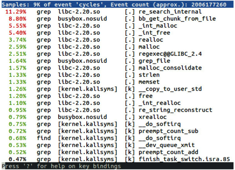
Figure 20.1 – perf report TUI

perf is able to record the kernel functions executed on behalf of the processes because it collects samples in kernel space.

The list is ordered with the most active functions first. In this example, all but one are captured while grep is running. Some are in a library, libc-2.20, some are in a program, busybox.nosuid, and some are in the kernel. We have symbol names for program and library functions because all the binaries have been installed on the target with debug information, and kernel symbols are being read from /boot/vmlinux. If you have vmlinux in a different location, add -k <path> to the perf report command. Rather than storing samples in perf.data, you can save them to a different file using perf record -o <file name> and analyze them using perf report -i <file name>.

By default, perf record samples at a frequency of 1,000 Hz using the cycles counter.

Tip

A sampling frequency of 1,000 Hz may be higher than you really need and
may be the cause of the observer effect. Try with lower rates; 100 Hz is enough for most cases, in my experience. You can set the sample frequency using
the -F option.

This is still not really making life easy; the functions at the top of the list are mostly low-level memory operations, and you can be fairly sure that they have already been optimized. Fortunately, perf record also gives us the ability to crawl up the call stack and see where these functions are being invoked.

Call graphs

It would be nice to step back and see the surrounding context of these costly functions. You can do that by passing the -g option to perf record to capture the backtrace from each sample.

Now, perf report shows a plus sign (+) where the function is part of a call chain. You can expand the trace to see the functions lower down in the chain:

Figure 20.2 – perf report (call graphs)

Important note

Generating call graphs relies on the ability to extract call frames from the stack, just as is necessary for backtraces in GDB. The information needed to unwind stacks is encoded in the debug information of the executables, but not all combinations of architecture and toolchains are capable of doing so.

Backtraces are nice, but where is the assembler, or better yet, the source code, for
these functions?

perf annotate

Now that you know which functions to look at, it would be nice to step inside and see the code and to have hit counts for each instruction. That is what perf annotate does, by calling down to a copy of objdump installed on the target. You just need to use perf annotate in place of perf report.

perf annotate requires symbol tables for the executables and vmlinux. Here is an example of an annotated function:

Figure 20.3 – perf annotate (assembler)

If you want to see the source code interleaved with the assembler, you can copy the relevant source files to the target device. If you are using the Yocto Project and build with the dbg-pkgs extra image feature, or have installed the individual -dbg package, then the source will have been installed for you in /usr/src/debug. Otherwise, you can examine the debug information to see the location of the source code:

$ arm-buildroot-linux-gnueabi-objdump --dwarf lib/libc-2.19.so | grep DW_AT_comp_dir

<3f> DW_AT_comp_dir : /home/chris/buildroot/output/build/hostgcc-initial-4.8.3/build/arm-buildroot-linux-gnueabi/libgcc

The path on the target should be exactly the same as the path you can see in
DW_AT_comp_dir.

Here is an example of annotation with the source and assembler code:

Figure 20.4 – perf annotate (source code)

Now we can see the corresponding C source code above cmp r0 and below the str r3, [fp, #-40] instruction.

This concludes our coverage of perf. While there are other statistical sampling profilers, such as OProfile and gprof, that predate perf, these tools have fallen out of favor in recent years, so I chose to omit them. Next, we will look at event tracers.

Tracing events

The tools we have seen so far all use statistical sampling. You often want to know more about the ordering of events so that you can see them and relate them to each other. Function tracing involves instrumenting the code with tracepoints that capture information about the event, and may include some or all of the following:

• A timestamp
• Context, such as the current PID
• Function parameters and return values
• A callstack

It is more intrusive than statistical profiling and it can generate a large amount of data. The latter problem can be mitigated by applying filters when the sample is captured and later on when viewing the trace.

I will cover three trace tools here: the kernel function tracers Ftrace, LTTng, and BPF.

Introducing Ftrace

The kernel function tracer Ftrace evolved from work done by Steven Rostedt and many others as they were tracking down the causes of high scheduling latency in real-time applications. Ftrace appeared in Linux 2.6.27 and has been actively developed since then. There are a number of documents describing kernel tracing in the kernel source in Documentation/trace.

Ftrace consists of a number of tracers that can log various types of activity in the kernel. Here, I am going to talk about the function and function_graph tracers and the event tracepoints. In Chapter 21, Real-Time Programming, I will revisit Ftrace and use it to show real-time latencies.

The function tracer instruments each kernel function so that calls can be recorded and timestamped. As a matter of interest, it compiles the kernel with the -pg switch to inject the instrumentation. The function_graph tracer goes further and records both the entry and exit of functions so that it can create a call graph. The event tracepoints feature also records parameters associated with the call.

Ftrace has a very embedded-friendly user interface that is entirely implemented through virtual files in the debugfs filesystem, meaning that you do not have to install any tools
on the target to make it work. Nevertheless, there are other user interfaces if you prefer: trace-cmd is a command-line tool that records and views traces and is available in Buildroot (BR2_PACKAGE_TRACE_CMD) and the Yocto Project (trace-cmd). There is a graphical trace viewer named KernelShark that is available as a package for the Yocto Project.

Like perf, enabling Ftrace requires setting certain kernel configuration options.

Preparing to use Ftrace

Ftrace and its various options are configured in the kernel configuration menu. You will need the following as a minimum:

• CONFIG_FUNCTION_TRACER from the Kernel hacking | Tracers | Kernel Function Tracer menu

For reasons that will become clear later, you would be well advised to turn on these options as well:

• CONFIG_FUNCTION_GRAPH_TRACER in the Kernel hacking | Tracers | Kernel Function Graph Tracer menu
• CONFIG_DYNAMIC_FTRACE in the Kernel hacking | Tracers | enable/disable function tracing dynamically menu

Since the whole thing is hosted in the kernel, there is no user space configuration to
be done.

Using Ftrace

Before you can use Ftrace, you have to mount the debugfs filesystem, which by convention goes in the /sys/kernel/debug directory:

# mount -t debugfs none /sys/kernel/debug

All the controls for Ftrace are in the /sys/kernel/debug/tracing directory; there is even a mini HOWTO in the README file there.

This is the list of tracers available in the kernel:

# cat /sys/kernel/debug/tracing/available_tracers

blk function_graph function nop

The active tracer is shown by current_tracer, which initially will be the null
tracer, nop.

To capture a trace, select the tracer by writing the name of one of the available_tracers to current_tracer, and then enable tracing for a short while, as shown here:

# echo function > /sys/kernel/debug/tracing/current_tracer

# echo 1 > /sys/kernel/debug/tracing/tracing_on

# sleep 1

# echo 0 > /sys/kernel/debug/tracing/tracing_on

In that one second, the trace buffer will have been filled with the details of every function called by the kernel. The format of the trace buffer is plain text, as described in Documentation/trace/ftrace.txt. You can read the trace buffer from the trace file:

# cat /sys/kernel/debug/tracing/trace

# tracer: function

#

# entries-in-buffer/entries-written: 40051/40051   #P:1

#

#                     _-----=> irqs-off

#                    / _----=> need-resched

#                   | / _---=> hardirq/softirq

#                   || / _--=> preempt-depth

#                   ||| /     delay

# TASK-PID   CPU#   ||||   TIMESTAMP   FUNCTION

#   | |       |     ||||       |          |

sh-361 [000] ...1 992.990646: mutex_unlock <-rb_simple_write

sh-361 [000] ...1 992.990658: __fsnotify_parent <-vfs_write

sh-361 [000] ...1 992.990661: fsnotify <-vfs_write

sh-361 [000] ...1 992.990663: __srcu_read_lock <-fsnotify

sh-361 [000] ...1 992.990666: preempt_count_add <-__srcu_read_lock

sh-361 [000] ...2 992.990668: preempt_count_sub <-__srcu_read_lock

sh-361 [000] ...1 992.990670: __srcu_read_unlock <-fsnotify

sh-361 [000] ...1 992.990672: __sb_end_write <-vfs_write

sh-361 [000] ...1 992.990674: preempt_count_add <-__sb_end_write

[…]

You can capture a large number of data points in just one second—in this case, over 40,000.

As with profilers, it is difficult to make sense of a flat function list like this. If you select the function_graph tracer, Ftrace captures call graphs like this:

# tracer: function_graph

#

# CPU  DURATION            FUNCTION CALLS

# |     |   |               |   |   |   |

0) + 63.167 us   |              } /* cpdma_ctlr_int_ctrl */

0) + 73.417 us   |            } /* cpsw_intr_disable */

0)               |            disable_irq_nosync() {

0)               |              __disable_irq_nosync() {

0)               |                __irq_get_desc_lock() {

0)   0.541 us    |                  irq_to_desc();

0)   0.500 us    |                  preempt_count_add();

0) + 16.000 us   |                }

0)               |                __disable_irq() {

0)   0.500 us    |                  irq_disable();

0)   8.208 us    |                }

0)               |                __irq_put_desc_unlock() {

0)   0.459 us    |                  preempt_count_sub();

0)   8.000 us    |                }

0) + 55.625 us   |              }

0) + 63.375 us   |            }

Now you can see the nesting of the function calls, delimited by braces, { and }. At the terminating brace, there is a measurement of the time taken in the function, annotated with a plus sign (+) if it takes more than 10 µs and an exclamation mark (!) if it takes more than 100 µs.

You are often only interested in the kernel activity caused by a single process or thread,
in which case you can restrict the trace to the one thread by writing the thread ID to
set_ftrace_pid.

Dynamic Ftrace and trace filters

Enabling CONFIG_DYNAMIC_FTRACE allows Ftrace to modify the function trace sites at runtime, which has a couple of benefits. Firstly, it triggers additional build-time processing of the trace function probes, which allows the Ftrace subsystem to locate them at boot time and overwrite them with NOP instructions, thus reducing the overhead of the function trace code to almost nothing. You can then enable Ftrace in production or near-production kernels with no impact on performance.

The second advantage is that you can selectively enable function trace sites rather than tracing everything. The list of functions is put into available_filter_functions; there are several tens of thousands of them. You can selectively enable function traces as you need them by copying the name from available_filter_functions to set_ftrace_filter and then stop tracing that function by writing the name to set_ftrace_notrace. You can also use wildcards and append names to the list. For example, suppose you are interested in tcp handling:

# cd /sys/kernel/debug/tracing

# echo "tcp*" > set_ftrace_filter

# echo function > current_tracer

# echo 1 > tracing_on

Run some tests and then look at trace:

# cat trace

# tracer: function

#

# entries-in-buffer/entries-written: 590/590   #P:1

#

#                     _-----=> irqs-off

#                    / _----=> need-resched

#                   | / _---=> hardirq/softirq

#                   || / _--=> preempt-depth

#                   ||| /     delay

#  TASK-PID   CPU# ||||   TIMESTAMP  FUNCTION

#    | |       |   ||||       |         |

dropbear-375 [000] ...1 48545.022235: tcp_poll <-sock_poll

dropbear-375 [000] ...1 48545.022372: tcp_poll <-sock_poll

dropbear-375 [000] ...1 48545.022393: tcp_sendmsg <-inet_sendmsg

dropbear-375 [000] ...1 48545.022398: tcp_send_mss <-tcp_sendmsg

dropbear-375 [000] ...1 48545.022400: tcp_current_mss <-tcp_send_mss

[…]

The set_ftrace_filter function can also contain commands, for example, to start and stop tracing when certain functions are executed. There isn't space to go into these details here, but if you want to find out more, read the Filter commands section in Documentation/trace/ftrace.txt.

Trace events

The function and function_graph tracers described in the preceding section record only the time at which the function was executed. The trace events feature also records parameters associated with the call, making the trace more readable and informative. For example, instead of just recording that the kmalloc function has been called, a trace event will record the number of bytes requested and the returned pointer. Trace events are used in perf and LTTng as well as Ftrace, but the development of the trace events subsystem was prompted by the LTTng project.

It takes effort from kernel developers to create trace events, since each one is different. They are defined in the source code using the TRACE_EVENT macro; there are over a thousand of them now. You can see the list of events available at runtime in /sys/kernel/debug/tracing/available_events. They are named subsystem:function, for example, kmem:kmalloc. Each event is also represented by a subdirectory in tracing/events/[subsystem]/[function], as demonstrated here:

# ls events/kmem/kmalloc

enable filter format id trigger

The files are as follows:

• enable: You write a 1 to this file to enable the event.
• filter: This is an expression that must evaluate to true for the event to be traced.
• format: This is the format of the event and parameters.
• id: This is a numeric identifier.
• trigger: This is a command that is executed when the event occurs using the syntax defined in the Filter commands section of Documentation/trace/ftrace.txt.

I will show you a simple example involving kmalloc and kfree. Event tracing does not depend on the function tracers, so begin by selecting the nop tracer:

# echo nop > current_tracer

Next, select the events to trace by enabling each one individually:

# echo 1 > events/kmem/kmalloc/enable

# echo 1 > events/kmem/kfree/enable

You can also write the event names to set_event, as shown here:

# echo "kmem:kmalloc kmem:kfree" > set_event

Now, when you read the trace, you can see the functions and their parameters:

# tracer: nop

#

# entries-in-buffer/entries-written: 359/359   #P:1

#

#                      _-----=> irqs-off

#                     / _----=> need-resched

#                    | / _---=> hardirq/softirq

#                    || / _--=> preempt-depth

#                    ||| /     delay

#   TASK-PID   CPU#  ||||    TIMESTAMP  FUNCTION

#      | |       |   ||||       |         |

     cat-382   [000] ...1  2935.586706: kmalloc:call_site=c0554644 ptr=de515a00

        bytes_req=384 bytes_alloc=512

        gfp_flags=GFP_ATOMIC|GFP_NOWARN|GFP_NOMEMALLOC

     cat-382   [000] ...1  2935.586718: kfree: call_site=c059c2d8 ptr=(null)

Exactly the same trace events are visible in perf as tracepoint events.

Since there is no bloated user space component to build, Ftrace is well-suited for deploying to most embedded targets. Next, we will look at another popular event tracer whose origins predate those of Ftrace.

Using LTTng

The Linux Trace Toolkit (LTT) project was started by Karim Yaghmour as a means of tracing kernel activity and was one of the first trace tools generally available for the Linux kernel. Later, Mathieu Desnoyers took up the idea and re-implemented it as a next-generation trace tool, LTTng. It was then expanded to cover user space traces as well as the kernel. The project website is at https://lttng.org/ and contains a comprehensive user manual.

LTTng consists of three components:

• A core session manager
• A kernel tracer implemented as a group of kernel modules
• A user space tracer implemented as a library

In addition to those, you will need a trace viewer such as Babeltrace (https://babeltrace.org) or the Eclipse Trace Compass plugin to display and filter the raw trace data on the host or target.

LTTng requires a kernel configured with CONFIG_TRACEPOINTS, which is enabled when you select Kernel hacking | Tracers | Kernel Function Tracer.

The description that follows refers to LTTng version 2.5; other versions may be different.

LTTng and the Yocto Project

You need to add these packages to the target dependencies to conf/local.conf:

IMAGE_INSTALL_append = " lttng-tools lttng-modules lttng-ust"

If you want to run Babeltrace on the target, also append the babeltrace package.

LTTng and Buildroot

You need to enable the following:

• BR2_PACKAGE_LTTNG_MODULES in the Target packages | Debugging, profiling and benchmark | lttng-modules menu
• BR2_PACKAGE_LTTNG_TOOLS in the Target packages | Debugging, profiling and benchmark | lttng-tools menu

For user space trace tracing, enable this:

• BR2_PACKAGE_LTTNG_LIBUST in the Target packages | Libraries | Other, enable lttng-libust menu

There is a package called lttng-babletrace for the target. Buildroot builds the babeltrace host automatically and places it in output/host/usr/bin/babeltrace.

Using LTTng for kernel tracing

LTTng can use the set of ftrace events described previously as potential tracepoints. Initially, they are disabled.

The control interface for LTTng is the lttng command. You can list the kernel probes using the following:

# lttng list --kernel

Kernel events:

-------------

writeback_nothread (loglevel: TRACE_EMERG (0)) (type: tracepoint)

writeback_queue (loglevel: TRACE_EMERG (0)) (type: tracepoint)

writeback_exec (loglevel: TRACE_EMERG (0)) (type: tracepoint)

[…]

Traces are captured in the context of a session, which in this example is called test:

# lttng create test

Session test created.

Traces will be written in /home/root/lttng-traces/test-20150824-140942

# lttng list

Available tracing sessions:

1) test (/home/root/lttng-traces/test-20150824-140942) [inactive]

Now enable a few events in the current session. You can enable all kernel tracepoints using the --all option, but remember the warning about generating too much trace data. Let's start with a couple of scheduler-related trace events:

# lttng enable-event --kernel sched_switch,sched_process_fork

Check that everything is set up:

# lttng list test

Tracing session test: [inactive]

    Trace path: /home/root/lttng-traces/test-20150824-140942

    Live timer interval (usec): 0

=== Domain: Kernel ===

Channels:

-------------

- channel0: [enabled]

Attributes:

      overwrite mode: 0

      subbufers size: 26214

      number of subbufers: 4

      switch timer interval: 0

      read timer interval: 200000

      trace file count: 0

      trace file size (bytes): 0

      output: splice()

Events:

      sched_process_fork (loglevel: TRACE_EMERG (0)) (type: tracepoint) [enabled]

      sched_switch (loglevel: TRACE_EMERG (0)) (type: tracepoint) [enabled]

Now start tracing:

# lttng start

Run the test load, and then stop tracing:

# lttng stop

Traces for the session are written to the session directory, lttng-traces/<session>/kernel.

You can use the Babeltrace viewer to dump the raw trace data in text format. In this case, I ran it on the host computer:

$ babeltrace lttng-traces/test-20150824-140942/kernel

The output is too verbose to fit on this page, so I will leave it as an exercise for you to capture and display a trace in this way. The text output from Babeltrace does have the advantage that it is easy to search for strings using grep and similar commands.

A good choice for a graphical trace viewer is the Trace Compass plugin for Eclipse, which is now part of the Eclipse IDE for the C/C++ developer bundle. Importing the trace data into Eclipse is characteristically fiddly. Briefly, you need to follow these steps:

1. Open the Tracing perspective.
2. Create a new project by selecting File | New | Tracing project.
3. Enter a project name and click on Finish.
4. Right-click on the New Project option in the Project Explorer menu and
   select Import.
5. Expand Tracing, and then select Trace Import.
6. Browse to the directory containing the traces (for example, test-20150824-140942), tick the box to indicate which subdirectories you want (it might be kernel), and click on Finish.
7. Expand the project and, within that, expand Traces[1], and then within that, double-click on kernel.

Now, let's switch gears away from LTTng and jump headfirst into the latest and greatest event tracer for Linux.

Using BPF

BPF (Berkeley Packet Filter) is a technology that was first introduced in 1992 to capture, filter, and analyze network traffic. In 2013, Alexi Starovoitov undertook a rewrite of BPF with help from Daniel Borkmann. Their work, then known as eBPF (extended BPF), was merged into the kernel in 2014, where it has been available since Linux 3.15. BPF provides a sandboxed execution environment for running programs inside the Linux kernel. BPF programs are written in C and are just-in-time (JIT) compiled to native code. Before that can happen, the intermediate BPF bytecode must first pass through a series of safety checks so that a program cannot crash the kernel.

Despite its networking origins, BPF is now a general-purpose virtual machine running inside the Linux kernel. By making it easy to run small programs on specific kernel and application events, BPF has quickly emerged as the most powerful tracer for Linux. Like what cgroups did for containerized deployments, BPF has the potential to revolutionize observability by enabling users to fully instrument production systems. Netflix and Facebook make extensive use of BPF across their microservices and cloud infrastructure for performance analysis and thwarting distributed denial of service (DDoS) attacks.

The tooling around BPF is evolving, with BPF Compiler Collection (BCC) and bpftrace establishing themselves as the two most prominent frontends. Brendan Gregg was deeply involved in both projects and has written about BPF extensively in his book BPF Performance Tools: Linux System and Application Observability, Addison-Wesley. With so many possibilities covering such a vast scope, new technology such as BPF can seem overwhelming. But much like cgroups, we don't need to understand how BPF works to start making use of it. BCC comes with several ready-made tools and examples that we can simply run from the command line.

Configuring the kernel for BPF

BCC requires a Linux kernel version of 4.1 or newer. At the time of writing, BCC only supports a few 64-bit CPU architectures, severely limiting the use of BPF in embedded systems. Fortunately, one of those 64-bit architectures is aarch64, so we can still run BCC on a Raspberry Pi 4. Let's begin by configuring a BPF-enabled kernel for that image:

$ cd buildroot

$ make clean

$ make raspberrypi4_64_defconfig

$ make menuconfig

BCC uses LLVM to compile BPF programs. LLVM is a very large C++ project, so it needs a toolchain with wchar, threads, and other features to build.

Tip

A package named ply (https://github.com/iovisor/ply) was merged into Buildroot on January 23, 2021, and should be included in the 2021.02 LTS release of Buildroot. ply is a lightweight, dynamic tracer for Linux that leverages BPF so that probes can be attached to arbitrary points in the kernel. Unlike BCC, ply does not rely on LLVM and has no required external dependencies aside from libc. This makes it much easier to port to embedded CPU architectures such as arm and powerpc.

Before configuring our kernel for BPF, let's select an external toolchain and modify raspberrypi4_64_defconfig to accommodate BCC:

1. Enable use of an external toolchain by navigating to Toolchain | Toolchain type | External toolchain and selecting that option.
2. Back out of External toolchain and open the Toolchain submenu. Select the most recent ARM AArch64 toolchain as your external toolchain.
3. Back out of the Toolchain page and drill down into System configuration | /dev management. Select Dynamic using devtmpfs + eudev.
4. Back out of /dev management and select Enable root login with password. Open Root password and enter a non-empty password in the text field.
5. Back out of the System configuration page and drill down into Filesystem images. Increase the exact size value to 2G so that there is enough space for the kernel source code.
6. Back out of Filesystem images and drill down into Target packages | Networking applications. Select the dropbear package to enable scp and ssh access to the target. Note that dropbear does not allow root scp and ssh access without a password.
7. Back out of Network applications and drill down into Miscellaneous target packages. Select the haveged package so programs don't block waiting for
   /dev/urandom to initialize on the target.
8. Save your changes and exit menuconfig.

Now, overwrite configs/raspberrypi4_64_defconfig with your menuconfig changes and prepare the Linux kernel source for configuration:

$ make savedefconfig

$ make linux-configure

The make linux-configure command will download and install the external toolchain and build some host tools before fetching, extracting, and configuring the kernel source code. At the time of writing, the raspberrypi4_64_defconfig from the 2020.02.9 LTS release of Buildroot still points to a custom 4.19 kernel source tarball from the Raspberry Pi Foundation's GitHub fork. Inspect the contents of your raspberrypi4_64_defconfig to determine what version of the kernel you are on. Once make linux-configure is done configuring the kernel, we can reconfigure it for BPF:

$ make linux-menuconfig

To search for a specific kernel configuration option from the interactive menu, hit / and enter a search string. The search should return a numbered list of matches. Entering a given number takes you directly to that configuration option.

At a minimum, we need to select the following to enable kernel support for BPF:

CONFIG_BPF=y

CONFIG_BPF_SYSCALL=y

We also need to add the following for BCC:

CONFIG_NET_CLS_BPF=m

CONFIG_NET_ACT_BPF=m

CONFIG_BPF_JIT=y

Linux kernel versions 4.1 to 4.6 need the following flag:

CONFIG_HAVE_BPF_JIT=y

Linux kernel versions 4.7 and later need this flag instead:

CONFIG_HAVE_EBPF_JIT=y

From Linux kernel version 4.7 onward, add the following so that users can attach BPF programs to kprobe, uprobe, and tracepoint events:

CONFIG_BPF_EVENTS=y

From Linux kernel version 5.2 onward, add the following for the kernel headers:

CONFIG_IKHEADERS=m

BCC needs to read the kernel headers to compile BPF programs, so selecting
CONFIG_IKHEADERS makes them accessible by loading a kheaders.ko module.

To run the BCC networking examples, we also need the following modules:

CONFIG_NET_SCH_SFQ=m

CONFIG_NET_ACT_POLICE=m

CONFIG_NET_ACT_GACT=m

CONFIG_DUMMY=m

CONFIG_VXLAN=m

Make sure to save your changes when exiting make linux-menuconfig so that they get applied to output/build/linux-custom/.config before building your BPF-enabled kernel.

Building a BCC toolkit with Buildroot

With the necessary kernel support for BPF now in place, let's add the user space libraries and tools to our image. At the time of writing, Jugurtha Belkalem and others have been working diligently to integrate BCC into Buildroot but their patches have yet to be merged. While an LLVM package has already been incorporated into Buildroot, there is no option to select the BPF backend needed by BCC for compilation. The new bcc and updated llvm package configuration files can be found in the MELP/Chapter20/ directory. To copy them over to your 2020.02.09 LTS installation of Buildroot, do the following:

$ cp -a MELP/Chapter20/buildroot/* buildroot

Now let's add the bcc and llvm packages to raspberrypi4_64_defconfig:

$ cd buildroot

$ make menuconfig

If your version of Buildroot is 2020.02.09 LTS and you copied the buildroot overlay from MELP/Chapter20 correctly, then there should now be a bcc package available under Debugging, profiling and benchmark. To add the bcc package to your system image, perform the following steps:

1. Navigate to Target packages | Debugging, profiling and benchmark and
   select bcc.
2. Back out of Debugging, profiling and benchmark and drill down into Libraries | Other. Verify that clang, llvm, and LLVM's BPF backend are all selected.
3. Back out of Libraries | Other and drill down into Interpreter languages and scripting. Verify that python3 is selected so that you can run the various tools and examples that come bundled with BCC.
4. Back out of Interpreter languages and scripting and select Show packages that are also provided by busybox under BusyBox from the Target packages page.
5. Drill down into System tools and verify that tar is selected for extracting the
   kernel headers.
6. Save your changes and exit menuconfig.

Overwrite configs/raspberrypi4_64_defconfig with your menuconfig changes again and build the image:

$ make savedefconfig

$ make

LLVM and Clang will take a long time to compile. Once the image is done building, use Etcher to write the resulting output/images/sdcard.img file to a micro SD card. Lastly, copy the kernel sources from output/build/linux-custom to a new /lib/modules/<kernel version>/build directory on the root partition of the micro SD card. This last step is critical because BCC needs access to the kernel source code to compile BPF programs.

Insert the finished micro SD into your Raspberry Pi 4, plug it into your local network with an Ethernet cable, and power the device up. Use arp-scan to locate your Raspberry Pi 4's IP address and SSH into it as root using the password you set in the previous section. I used temppwd for the root password in the configs/rpi4_64_bcc_defconfig that I included with my MELP/Chapter20/buildroot overlay. Now, we are ready to gain some firsthand experience of experimenting with BPF.

Using BPF tracing tools

Doing almost anything with BPF, including running the BCC tools and examples, requires root privileges, which is why we enabled root login via SSH. Another prerequisite is mounting debugfs as follows:

# mount -t debugfs none /sys/kernel/debug

The directory where the BCC tools are located is not in the PATH environment, so navigate there for easier execution:

# cd /usr/share/bcc/tools

Let's start with a tool that displays the task on-CPU time as a histogram:

# ./cpudist

cpudist shows how long tasks spent on the CPU before being descheduled:

Figure 20.5 – cpudist

If instead of a histogram you see the following error, then you forgot to copy the kernel sources to the micro SD card:

modprobe: module kheaders not found in modules.dep

Unable to find kernel headers. Try rebuilding kernel with CONFIG_IKHEADERS=m (module) or installing the kernel development package for your running kernel version.

chdir(/lib/modules/4.19.97-v8/build): No such file or directory

[…]

Exception: Failed to compile BPF module <text>

Another useful system-wide tool is llcstat, which traces cache reference and cache miss events and summarizes them by PID and CPU:

Figure 20.6 – llcstat

Not all BCC tools require us to hit Ctrl + C to end. Some such as llcstat take a sample period as a command-line argument.

We can get more specific and zoom in on specific functions using tools such as funccount, which takes a pattern as a command-line argument:

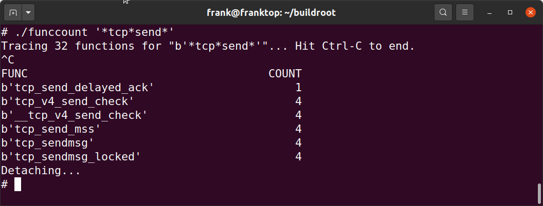
Figure 20.7 – funccount

In this instance, we are tracing all kernel functions containing tcp followed by send in their names. Many BCC tools can also be used to trace functions in user space. That requires either debug symbols or instrumenting the source code with user statically defined tracepoint (USDT) probes.

Of special interest to embedded developers are the hardirqs tools, which measure the time spent in the kernel servicing hard interrupts:

Figure 20.8 – hardirqs

Writing your own general-purpose or custom BCC tracing tools in Python is easier than you might expect. You can find several examples to read and fiddle with in the /usr/share/bcc/examples/tracing directory that comes with BCC.

This concludes our coverage of Linux event tracing tools: Ftrace, LTTng, and BPF. All of them require at least some kernel configuration to work. Valgrind offers more profiling tools that operate entirely from the comfort of user space.

Using Valgrind

I introduced Valgrind in Chapter 18, Managing Memory, as a tool for identifying memory problems using the memcheck tool. Valgrind has other useful tools for application profiling. The two I am going to look at here are Callgrind and Helgrind. Since Valgrind works by running the code in a sandbox, it can check the code as it runs and report certain behaviors, which native tracers and profilers cannot do.

Callgrind

Callgrind is a call graph-generating profiler that also collects information about processor cache hit rate and branch prediction. Callgrind is only useful if your bottleneck is CPU-bound. It's not useful if heavy I/O or multiple processes are involved.

Valgrind does not require kernel configuration, but it does need debug symbols.
It is available as a target package in both the Yocto Project and Buildroot
(BR2_PACKAGE_VALGRIND).

You run Callgrind in Valgrind on the target like so:

# valgrind --tool=callgrind <program>

This produces a file called callgrind.out.<PID>, which you can copy to the host and analyze with callgrind_annotate.

The default is to capture data for all the threads together in a single file. If you add the --separate-threads=yes option when capturing, there will be profiles for each of the threads in files named callgrind.out.<PID>-<thread id>, for example, callgrind.out.122-01 and callgrind.out.122-02.

Callgrind can simulate the processor L1/L2 cache and report on cache misses. Capture the trace with the --simulate-cache=yes option. L2 misses are much more expensive than L1 misses, so pay attention to code with high D2mr or D2mw counts.

The raw output from Callgrind can be overwhelming and difficult to untangle. A visualizer such as KCachegrind (https://kcachegrind.github.io/html/Home.html) can help you navigate the mountains of data Callgrind collects.

Helgrind

Helgrind is a thread-error detector for detecting synchronization errors in C, C++, and Fortran programs that include POSIX threads.

Helgrind can detect three classes of errors. Firstly, it can detect the incorrect use of the API. Some examples are unlocking a mutex that is already unlocked, unlocking a mutex that was locked by a different thread, or not checking the return value of certain pthread functions. Secondly, it monitors the order in which threads acquire locks to detect cycles that may result in deadlocks (also known as the deadly embrace). Finally, it detects data races, which can happen when two threads access a shared memory location without using suitable locks or other synchronization to ensure single-threaded access.

Using Helgrind is simple; you just need this command:

# valgrind --tool=helgrind <program>

It prints problems and potential problems as it finds them. You can direct these messages to a file by adding --log-file=<filename>.

Callgrind and Helgrind rely on Valgrind's virtualization for their profiling and deadlock detection. This heavyweight approach slows down the execution of your programs, increasing the likelihood of the observer effect.

Sometimes the bugs in our programs are so reproducible and easy to isolate that a simpler, less invasive tool is enough to quickly debug them. That tool more often than not is strace.

Using strace

I started the chapter with a simple and ubiquitous tool, top, and I will finish with another: strace. It is a very simple tracer that captures system calls made by a program and, optionally, its children. You can use it to do the following:

• Learn which system calls a program makes.
• Find those system calls that fail, together with the error code. I find this useful
  if a program fails to start but doesn't print an error message or if the message is
  too general.
• Find which files a program opens.
• Find out which syscalls a running program is making, for example, to see whether it is stuck in a loop.

There are many more examples online; just search for strace tips and tricks. Everybody
has their own favorite story, for example, https://alexbilson.dev/posts/strace-debug/.

strace uses the ptrace(2) function to hook calls as they are made from user space to the kernel. If you want to know more about how ptrace works, the manual page is detailed and surprisingly readable.

The simplest way to get a trace is to run the command as a parameter to strace, as shown here (the listing has been edited to make it clearer):

# strace ./helloworld

execve("./helloworld", ["./helloworld"], [/* 14 vars */]) = 0

brk(0)                                  = 0x11000

uname({sys="Linux", node="beaglebone", ...}) = 0

mmap2(NULL, 4096, PROT_READ|PROT_WRITE, MAP_PRIVATE|MAP_ANONYMOUS, -1, 0) = 0xb6f40000

access("/etc/ld.so.preload", R_OK)      = -1 ENOENT (No such file or directory)

open("/etc/ld.so.cache", O_RDONLY|O_CLOEXEC) = 3

fstat64(3, {st_mode=S_IFREG|0644, st_size=8100, ...}) = 0

mmap2(NULL, 8100, PROT_READ, MAP_PRIVATE, 3, 0) = 0xb6f3e000

close(3)                                = 0

open("/lib/tls/v7l/neon/vfp/libc.so.6", O_RDONLY|O_CLOEXEC) = -1

ENOENT (No such file or directory)

[...]

open("/lib/libc.so.6", O_RDONLY|O_CLOEXEC) = 3

read(3,

"177ELF1113(1$`1004"...,

512) = 512

fstat64(3, {st_mode=S_IFREG|0755, st_size=1291884, ...}) = 0

mmap2(NULL, 1328520, PROT_READ|PROT_EXEC, MAP_PRIVATE|MAP_DENYWRITE,

3, 0) = 0xb6df9000

mprotect(0xb6f30000, 32768, PROT_NONE)  = 0

mmap2(0xb6f38000, 12288, PROT_READ|PROT_WRITE,

MAP_PRIVATE|MAP_FIXED|MAP_DENYWRITE, 3, 0x137000) = 0xb6f38000

mmap2(0xb6f3b000, 9608, PROT_READ|PROT_WRITE,

MAP_PRIVATE|MAP_FIXED|MAP_ANONYMOUS, -1, 0) = 0xb6f3b000

close(3)

[...]

write(1, "Hello, world! ", 14Hello, world!

    )         = 14

exit_group(0)                           = ?

+++ exited with 0 +++

Most of the trace shows how the runtime environment is created. In particular, you can see how the library loader hunts for libc.so.6, eventually finding it in /lib. Finally, it gets to running the main() function of the program, which prints its message and exits.

If you want strace to follow any child processes or threads created by the original process, add the -f option.

Tip

If you are using strace to trace a program that creates threads, you almost certainly want to use the -f option. Better still, use -ff and -o <file name> so that the output for each child process or thread is written to a separate file named <filename>.<PID | TID>.

A common use of strace is to discover which files a program tries to open at startup. You can restrict the system calls that are traced through the -e option, and you can write the trace to a file instead of stdout using the -o option:

# strace -e open -o ssh-strace.txt ssh localhost

This shows the libraries and configuration files ssh opens when it is setting up
a connection.

You can even use strace as a basic profile tool. If you use the -c option, it accumulates the time spent in system calls and prints out a summary like this:

# strace -c grep linux /usr/lib/* > /dev/null

% time     seconds  usecs/call     calls    errors syscall

------ ----------- ----------- --------- --------- ----------

78.68    0.012825         1       11098      18    read

11.03    0.001798         1        3551            write

10.02    0.001634         8         216      15    open

  0.26    0.000043         0         202            fstat64

  0.00    0.000000         0         201            close

  0.00    0.000000         0          1             execve

  0.00    0.000000         0          1       1     access

  0.00    0.000000         0          3             brk

  0.00    0.000000         0         199            munmap

  0.00    0.000000         0          1             uname

  0.00    0.000000         0          5             mprotect

  0.00    0.000000         0         207            mmap2

  0.00    0.000000         0         15       15    stat64

  0.00    0.000000         0          1             getuid32

  0.00    0.000000         0          1             set_tls

------ ----------- ----------- --------- --------- -----------

100.00    0.016300                 15702      49 total

strace is extremely versatile. We have only scratched the surface of what the tool can do. I recommend downloading Spying on your programs with strace, a free zine by Julia Evans available at https://wizardzines.com/zines/strace/.

Summary

Nobody can complain that Linux lacks options for profiling and tracing. This chapter has given you an overview of some of the most common ones.

When faced with a system that is not performing as well as you would like, start with top and try to identify the problem. If it proves to be a single application, then you can use perf record/report to profile it, bearing in mind that you will have to configure the kernel to enable perf and you will need debug symbols for the binaries and kernel. If the problem is not so well localized, use perf or BCC tools to get a system-wide view.

Ftrace comes into its own when you have specific questions about the behavior of the kernel. The function and function_graph tracers provide a detailed view of the relationship and sequence of function calls. The event tracers allow you to extract more information about functions, including the parameters and return values. LTTng performs a similar role, making use of the event trace mechanism, and adds high-speed ring buffers to extract large quantities of data from the kernel. Valgrind has the advantage of running code in a sandbox and can report on errors that are hard to track down in other ways. Using the Callgrind tool, it can generate call graphs and report on processor cache usage, and with Helgrind, it can report on thread-related problems.

Finally, don't forget strace. It is a good standby for finding out which system calls a program is making, from tracking file open calls to finding file pathnames and checking for system wake-ups and incoming signals.

All the while, be aware of, and try to avoid, the observer effect; make sure that the measurements you are making are valid for a production system. In the next chapter, I
will continue with this theme as we delve into the latency tracers that help us quantify the real-time performance of a target system.

Further reading

I highly recommend Systems Performance: Enterprise and the Cloud, Second Edition, and BPF Performance Tools: Linux System and Application Observability, both by Brendan Gregg.