
Viral Outbreaks and Blood Clots
9.1 Background
The setting is a crowded schoolroom in winter where one child after another comes down with a rash and fever, a case of measles. From time to time, epidemics of childhood diseases such as measles arise in cities around the country, most recently during the late 1980s. Susceptible individuals fall victim to a contagious disease when they encounter others who are already infected. There is a whole class of problems in which two or more species interact that can be formulated mathematically in quite similar ways. Grim warfare, territorial disputes, the hide-and-seek behavior of predators and their victims, and even chemical reactions are all manifestations of species that affect each other because they are in the same place at the same time.
What the mathematical models of these processes have in common is that they record changes that take place over time and are described in terms of rates of change, such as the rate of reproduction and the rate of becoming infected. But rates imply derivatives, so it is not surprising that the models are expressed as differential equations, enough so that we can gain some insight into an assortment of models. In addition to using analytical tools to reveal the behavior of solutions to the differential equations, it is expedient to employ computer-generated graphics to display the numerically integrated solutions. This will be done throughout this chapter and the next.
The epidemic model itself is discussed in Section 9.2, and in Sections 9.3 and 9.4 we obtain a brief glimpse of chaotic dynamics in two different settings.
Another illustration of these ideas is the interplay of excitation and inhibition that is common in any number of living systems. A striking example is provided by blood coagulation, in which the breaking of a blood vessel mobilizes a cascade of enzyme reactions that lead to the rapid formation of a clot to plug the lesion. Without this, one would bleed to death. However, an unchecked production of clots can also be fatal, and so the biochemical reactions include inhibitors that serve to brake the possibility of a runaway system. It is the delicate balance between these competing requirements that enables the blood-clotting system to work as well as it generally does. This topic is taken up in Section 9.7, while in Sections 9.5 and 9.6 we consider other excitable dynamics that are manifested, in one instance by the onset of algal blooms and in the other by the viral contamination of alga cells.
Episodes of algae growth have been recorded in estuaries and coastal areas for several hundred years, and most have been considered to be benign events or, at worst, mild nuisances that recur with humdrum regularity in late spring and summer. However, in recent years there have been more sporadic, less predictable, and certainly more severe bouts of elevated cell growth of certain toxic algae species, known generically as red tides or even brown tides. There is a mounting worldwide concern for these unusual bloom episodes because of their adverse impact on fisheries and aquaculture and from the eutrophication that results from their collapse. These harmful marine flare-ups are marked by a sudden proliferation of cell counts followed, quite often, by rapid disintegration.
The onset of the outbreaks can be attributed, in part, to a confluence of climatic and meteorological conditions that alter the physical and chemical composition of the waters in such a way as to predispose one algal species to achieve dominance, in preference to other species that normally inhabit the same territory. The intruder may arrive as a castaway in ship ballast or from a storm event far out at sea, and it seizes the opportunity for unbridled growth when the local conditions are favorable. However, even if bloom initiation is largely due to chance events, its subsequent duration and severity are moderated by other organisms, the zooplankton, that graze on the algae. A simple model of this prey–grazer interaction is treated in Section 9.5, offering a plausible metaphor for the observed dynamics of a bloom in progress, while in Section 9.6 we consider a specific mechanism of bloom disintegration caused by viral infection of the algae cells.
What algae blooms, infectious diseases, and blood clotting have in common is that these events are triggered whenever a certain threshold in favorable conditions is attained, such as a salinity level high enough for the algae, a critical level of infectives, or activation of an enzyme cascade that leads to blood clotting. These are all examples of what are called excitable systems that remain quiescent until suddenly ignited by propitious events.
9.2 Measles Epidemics
Our intention is to model childhood epidemics such as measles, chickenpox, and mumps to track the dynamics of outbreaks of these contagious diseases.
We begin by dividing up the population of a given region into four categories: susceptibles—those individuals who are able to contract the communicable disease; exposed—infected people who are not yet able to transmit the disease to others; infectives—those who are capable of spreading the disease; and recovered.
With childhood illnesses it is largely true that a recovered person becomes permanently immune, and so the last category includes individuals who are immune to begin with or who succumb to the disease. Let’s denote the fractions of susceptible, exposed, infective, and recovered in the population by S, E, I, and R, respectively. We assume that all newborns are susceptibles at birth and that the population size remains constant by balancing births, on one hand, to deaths and emigrations, on the other. The diseases are endemic, in the sense of recurring from year to year, with varying severity. As susceptibles become ill and, ultimately, immune or dead, their supply is replenished by newborns, and so the model must include birth rates explicitly. Later we consider what happens in virulent diseases whose contagion is so rapid that they run their course within a time span so short that the addition of fresh susceptibles can be disregarded.
We denote by b the disease contact rate, which is the average number of effective disease transmissions per unit time per infective. This requires a word of explanation. The disease is transmitted in proportion to the number of possible encounters between infectives and susceptibles, which means that b is the average rate at which an infective comes into contact with another person, so bI is the total contact rate. This has to be multiplied by the likelihood that the person contacted is in fact a noninfective, which equals S, the fraction of susceptibles in the population. It is assumed that b increases with the total population size, since the number of contacts is greater in dense urban areas than in sparse rural aggregations. This situation may not prevail, however, when the number of susceptibles is in large excess over the quantity of infectives. Increasing S in this case has little or no effect on the number of contacts made by an infective, and the limiting factor now for disease transmission is only the size of I.
Let r be the average birth rate (1/r is therefore the average life expectancy). Then
![]() (9.1)
(9.1)
models the rate of change of S. The second term on the right expresses the fact that, because total population is constant, susceptibles are removed by death and emigration at the same rate r at which they enter the population.
The class of exposed individuals increases over time at a rate equal to the rate at which susceptibles become infected, namely, bSI. They disappear from the population at a rate rE, due to death and emigration, and at a rate aE, where a is the average number of exposed people that become contagious per unit time. The reciprocal, 1/a, is, therefore, the mean latency period during which the disease incubates prior to becoming infectious. Putting this together gives the equation
![]() (9.2)
(9.2)
The infectives are now seen to increase at a rate aE and to be removed at rates rI (for the same reason as before) and cI, where c is the average number of infected people that recover per unit time; the reciprocal, 1/c, is then the mean infectious period. Thus
![]() (9.3)
(9.3)
Finally, the recovered class evidently increases at a rate cI and disappears at rate rR:
![]() (9.4)
(9.4)
The four coupled equations describe the epidemic model but are too formidable to handle with the tools at our disposal. To get some idea of the behavior of the solution to this system, we simplify a bit and ignore the class E by assuming that the latency period is zero. This means that susceptibles are immediately infected, and so Equation (9.3) for I′ needs to be replaced by
![]()
Three equations remain:
 (9.5)
(9.5)
The first two equations are independent of R, so we can simplify further by retaining only these two. Because S + I + R = 1, the value of R is obtained from a knowledge of S and I. Thus
![]() (9.6)
(9.6)
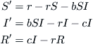
We surmise that there are oscillatory solutions about the equilibrium state defined by S = (r + c)/b, I = r (b – r – c)/b(r + c) to describe the waxing and waning of real epidemics. The quantity (r + c)/b is taken to be less than 1 to guarantee that I is positive at the equilibrium. Therefore, if the ratio of the recovery rate c to the contact rate b is small enough, the epidemic can be sustained. This implies that intervention on the part of public health officials can have an impact on the severity or even the likelihood of an epidemic. For example, inoculation of school children reduces the number of susceptibles, while quick isolation of infectives increases the removal rate c.
The trajectories for a typical case were generated by computer and are shown in Figure 9.1. We observe that the oscillations wind down to a point attractor as the number of infectives moves up and down. A numerical integration of the full set of Equations (9.1) to (9.4) would reveal a similar pattern of damped oscillations, which appears to indicate a cyclic recurrence of outbreaks with diminishing severity.
The Jacobean for Equations (9.6) at the equilibrium values of S and I is calculated quite simply and is given by
![]()
From this we see that the equilibrium is indeed an attractor. Also, the eigenvalues are complex, which indicates oscillatory solutions and this is what Figure 9.1 shows.
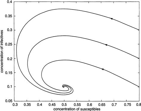
The actual data on measles shows a different pattern, in which the disease recurs with levels of severity that fluctuate erratically from year to year. In New York City, for example, consider measles outbreaks from 1928 to 1963 (when large-scale vaccination of schoolchildren began); the monthly data on measles cases exhibits irregular peaks and troughs that appear to have two-year cycles of highs and lows (Figure 9.2).
There are several possible reasons for the discrepancy between what the model predicts and what one observes. The most compelling, perhaps, is that the parameter b, the rate at which the disease is transmitted, need not be constant and can, in fact, vary widely. The disease pathogen appears to be more virulent during winter months, at a time when children are confined together in school; contact is not as close and is less frequent during the summer months. With this in mind, the parameter b can be replaced in the model by a periodic function having a period of 1 year, with a low value in July and a high value in February:
![]()
where b0 is the average contact rate and b1, a number between zero and 1, measures the magnitude of the seasonal effect. The time t = 0 represents the beginning of February. With b(t) substituted into the equations in place of a constant b, the original model can be integrated numerically to give solutions that indeed mimic the data seen in New York City and elsewhere for actual measles outbreaks. In certain parameter regimes, in fact, the periodically forced solutions are indistinguishable from random fluctuations, a phenomenon that some authors describe as a manifestation of chaotic dynamics, in which, loosely speaking, the trajectories settle down to a complicated attractor in state space that is neither a point nor a cycle. More will be said about chaotic dynamics in the next section.
It is important to note that all the parameters in the model, namely, r, b, b0, and c, are statistical averages from actual data, so the equilibrium values of S and I are also averages. However, stochastic fluctuations in the actual values of these variables can be significant when the actual values of the variables are quite small. If the number of infectives is low, for instance, a chance fluctuation could reduce it to zero. In this case, the epidemic is extinguished, a condition known as fade-out. This can also be seen during those periods in which a contagious disease is waning, because the number of susceptibles has decreased sufficiently that the rate of arrival of new susceptibles is not fast enough to compensate for the die-off or immunity rate of the infectives. Random events can exacerbate this situation by the sudden removal of people during one of the troughs in a wax-and-wane cycle, with the consequence of quenching the transmission of disease. For these reasons it is generally assumed, for measles anyway, that the population of susceptibles is substantial. It is known, in fact, that measles cannot remain endemic in communities with much fewer than a million people.
When an epidemic comes and goes quickly in one cycle, the influx of new susceptibles can be neglected in the model Equations (9.6) by choosing r to be zero. Looking at the sign of the derivative in the equation for I (when r is zero) shows that the number of infectives is on the rise only when the initial fraction of susceptibles is greater than c/b. This is called a threshold condition, because above it there is an initial increase in the number of contagious individuals, whereas below it the epidemic does not ignite. This is quite similar to what happens in the autocatalytic model of a biochemical reaction, which will be discussed in Section 9.7 (see also the comments in Section 9.8).
9.3 Chaotic Dynamics or Randomness?
Let’s return now to the measles model of the preceding section, which was found to be wanting because it failed to mimic actual measles events from year to year in a city like New York. It was suggested there that more realistic results could be obtained by making the contact rate b into a periodic function to simulate seasonal effects.
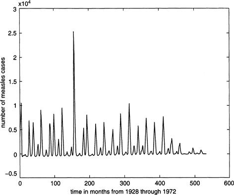
Figure 9.3a shows the fraction I of infective cases over a 30-year period as obtained from an integration of the periodically forced Equations (9.1) through (9.4). The parameters in the model are estimated from census data and medical records as r = .02 per year, b0 = 1,800 per year, a = 35.58 per year, c = 100 per year, and b1 = .285. The severity of the outbreaks varies erratically from year to year and resembles that found in the actual New York City data from 1928 to 1963, during which the epidemic peaked at about 25,000 cases a year (Figure 9.2). With a total population of about 6 million, this corresponds to a maximum fraction of infectives of roughly .004, as shown in Figures 9.3a and b.
FIGURE 9.3 The fraction of infectives over a 30-year period from the periodically forced model Equations (9.1) through (9.4), with b1 = 0.285.
The only difference between panels a and b is that the initial values of susceptibles S differs by 0.00001, with all other model parameters remaining the same. The resulting orbits demonstrate a sensitivity to initial conditions, a signature of chaotic dynamics.
The solutions of the model equations have evidently settled down to an attractor that is clearly recurrent from year to year, but the magnitude of the fluctuations is somewhat unpredictable. Either this is a manifestation of a cyclic attractor’s having a very long period of motion, or it may represent what is known as a chaotic attractor. There are two important signatures of a chaotic attractor, or, more simply, chaos. One of these is an extreme sensitivity to initial conditions, meaning that small changes in initial values of any of the variables produces solutions that rapidly diverge from each other over time. This evidently cannot happen on a periodic attractor. The other attribute of chaos is that orbits will move arbitrarily close to every point on the attractor infinitely often. The time lapse between successive returns is erratic, however. This recurrent behavior differs from that of a periodic attractor because the orbits weave a complex tangle in which the orbits never cross themselves (if they did intersect, the uniqueness principle would force the trajectory to be a closed path on which motion is periodic).
To illustrate the idea of sensitivity, let us change the initial value of S by only 0.0001 from the value used to obtain Figure 9.3a. All other initial values for I, E, and R remain the same. The result is shown in Figure 9.3b, where we see that the solution remains roughly the same for a while to the one shown in the figure above it, but soon it changes dramatically so that by the time 30 years has elapsed the value of I is evolving along a completely different part of the attractor. Moreover, although there are annual measles outbreaks, the magnitude of the fluctuations in the number of infectives is unpredictable, and the time between nearly recurrent events appears to be essentially random. This shows that we can never hope to replicate exactly the actual dynamics of a chaotic process, and the solutions illustrate only what the typical behavior is like.
These numerical results are still somewhat unsatisfactory, however, since the actual New York City data from 1945 onward exhibits alternating highs and lows in the number of reported cases of measles, with a severe outbreak in one year followed by a mild incidence of disease in the subsequent year. The problem is that the parameter b1 that measures the effect of seasonality is not known exactly, and even a slight change in its value can have a notable effect in the computational results. For example, a change to b1 = 0.275 gives alternating biannual peaks in the number of cases, as shown in Figure 9.4, which is more consistent with the data from 1945 onward but, on the other hand, doesn’t reach the reported levels of severity that were visible in Figure 9.3, where b1 = 0.285.
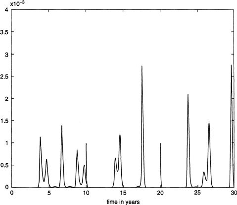
FIGURE 9.4 Fraction of infectives over a 30-year period from the periodically forced model Equations (9.1) through (9.4), with b1 = 0.275.
Although the model is a plausible caricature of the actual dynamics of a recurrent epidemic, it is at least arguable whether an alternative formulation would not be more convincing. One can allow the parameters to vary at random, for example, to represent chance variations, as in the wayward movement of infectives into and out of the region. Chance events that disturb the rhythm of periodic dynamics sometimes can give the appearance of chaos, and some systems modeled by three or more differential equations have attractors that are not quite periodic, but nevertheless an appearance of recurrence is maintained, in the sense that the orbit returns to nearby points infinitely often, weaving a complex “stretch and fold” pattern in some confined region of space.
Attractors for certain biological systems seem to behave this way either because the motion represented by a cycle loops around for a very long time before returning to its starting point or because the limiting behavior consists of fluctuations that appear random. Indeed, the populations of many species exhibit erratic fluctuations, and, although some of the recurrence that one observes may be due partially to an internal dynamic that determines the interactions with other species and its environment, there may also be a component of chance. As we saw in the case of measles, it is difficult to distinguish in an unambiguous manner whether one is dealing with deterministic chaos or noise contamination that masks the biological interactions. Although the footprints of chaos can be partially discerned in some data sets, a clear marker is still lacking.
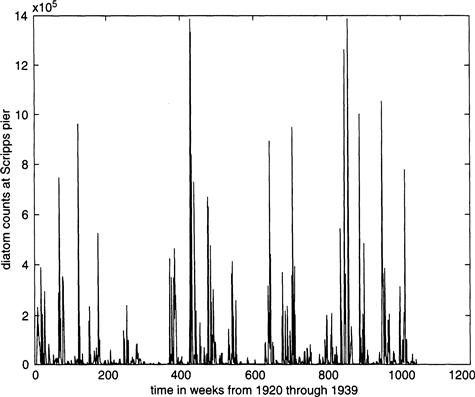
Another example of this ambiguity, besides that of measles, is connected to the tiny marine diatoms that populate many water bodies. Figure 9.5 shows the weekly average diatom count over a span of 20 years as measured near the pier of the Scripps Institute in La Jolla, California. There are several known and conjectured influences on the rise and fall of the diatom counts, including changes in temperature and salinity, the upwelling of nutrients from deeper waters, and the effects of predation. Nonetheless, the haphazard fluctuations recorded in Figure 9.5 may be a manifestation of randomness as much as of any orderly underlying process.
The allure of chaos is that it enables us to think of complex fluctuations as a deterministic process described by differential equations, even when the observed motion appears to be the result of random noise superimposed on some orderly process.
9.4 Predator-Mediated Coexistence
As a follow-up to the discussion in the previous section, I want to provide a cautionary tale in ecology by presenting a somewhat-contrived one-predator, two-prey model that supplies a metaphor for the idea that species diversity in competitive communities can be enhanced by the presence of a predator that mediates the interaction between two competitors. More specifically, if one of a pair of prey species becomes extinct because it dominates the other, then a predator can exert pressure on the stronger and more abundant species, reducing the advantage it has on its competitor, and this opens the possibility for the coexistence of both (indeed, all three) of the species. Two specific examples of this include the removal of feral cats from an Australian Island to save the native seabirds. However, this allowed the rabbit population to explode, destroying much of the fragile vegetation that the birds depend on for cover (“Removing Cats to Protect Birds Backfires on Island,” New York Times, Jan. 13, 2009). Another example concerns the overfishing of sharks in the northwest Atlantic, allowing intermediate predators to deplete bay scallop beds (see Fountain, “Study finds Shark Overfishing May Lower Scallop Population,” New York Times, March 31, 2007, and Myers and Peterson, “Cascading Effects of the Loss of Apex Predator Sharks from a Coastal Ocean,” Science 315, 2007, pp. 1846–1850).
The model equations are:
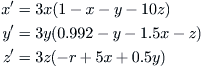 (9.7)
(9.7)
in which x, y, and z are, respectively, the population densities of the dominant competitor, the weaker competitor, and the top predator.
As the attrition rate r of the predator decreases as more prey become available, a single attracting equilibrium in which the weaker competitor becomes extinct bifurcates into a periodic orbit in which all three species coexist. This appears to be an example of a Hopf bifurcation, as discussed in the previous chapter. With further decreases of this parameter, more complicated periodic behavior and ultimately chaotic dynamics ensue. This last case is seen in Figure 9.6, in which r = 0.9. When r = 1.2 there is a single cyclic solution, as illustrated in Figure 9.7. Here we see a weaving pattern among the three species on top and then a temporal history of the dominant prey species below, in which it is seen to wax and wane over time. However, as discussed in Section 9.3, in an actual multitiered predator–prey system, the complicated oscillatory behavior one observes may be as much an indication of environmental noise overlaying the dynamics of the species as a bona fide example of chaos in the mathematical sense.
FIGURE 9.6 Integration of Equations 9.7 for r = 0.90.
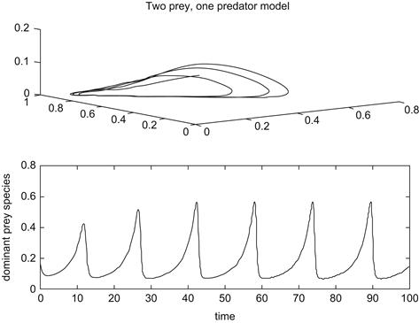
FIGURE 9.7 Integration of Equations 9.7 for r = 1.2.
9.5 An Unusual Bloom
Since 1985, a small (2–3 μm in diameter) algae called Aureococcus anophagefferens or, simply, A.a., has sporadically erupted in the Peconic estuary and nearby embayments of eastern Long Island, New York. The commercial harvesting of scallops and mussels is seriously disrupted during one of these blooms because the shellfish cannot ingest A.a., and they therefore starve. Cell counts of A.a. catapult within days to over 106 cells/liter, and even as high as 109 in at least one year, leaving the waters an impenetrable muddy haze called a “brown tide.”
Certain microzooplankton, small crustaceans, feed on A.a. and other tiny algae that are generically classified as phytoplankton. This trophic link between the zooplankton and their prey can be modeled, in the simplest case, by a pair of differential equations in the variables x and y, where x is the concentration of A.a., in units of 105 cells per liter, and y is the concentration of the grazing zooplankton, in units of 103 per liter. The equations are written first, and then the individual terms are described in more detail:
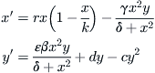 (9.8)
(9.8)
The growth rate of the prey is taken to be logistic, with a theoretically maximum sustainable population density of k that ranges from 20 to 30 (in units of 105 cells per liter, as already noted), and the per capita growth rate r is calibrated to correspond to one to two cell divisions per day at the height of a bloom. The value of k will change according to local environmental factors that serve to either trigger or inhibit a bloom. This will also be true of r because the cell-division rate is temperature-dependent and therefore varies with the climate.
The grazing rate is estimated at about 0.5 cells per liter per day, a figure used in setting the predation rate γ in the model. The quantity β is a fraction that measures the conversion of ingested cells into zooplankton biomass and is roughly 0.4.
The quantity ε is a small constant to ensure a correspondingly small variation in y compared to x. This says that changes in y are “slow” as compared to “fast” changes in x.
The form of the predation term requires some explanation. At the very beginning of a bloom, grazing is negligible because of the availability of alternative and preferable food sources. But, as the bloom progresses, the zooplankton shift their attention to A.a. because it is becoming an abundant and even dominant species. Also, at high population densities, there is an increasing rate of algal mortality caused by viruses that lyse the cells and hasten bloom disintegration. This means the growth is proportional to x2 instead of just x because x2 increases slowly at first and much more rapidly when x is at elevated levels. The denominator serves to measure satiation of the grazer as x becomes abundant: When x is large, the predation term is essentially proportional to y alone, whereas for small-to-moderate x, it depends on the interaction between both predator and prey. As the parameter δ decreases, satiation takes place more rapidly.
The quantity d is a per capita growth rate of grazers due to the availability of alternative food sources, and cy2 is a death rate that increases with y2 to signal the combined effects of increased predation by larger “macrozooplankton,” such as copepods, on the smaller zooplankton as the latter become more abundant, as well as more aggressive competition and interference among the various species of feeding microzooplankton. In effect, this term is a surrogate for a three-tiered trophic chain that includes two different levels of predators. The parameters δ, d, and c were calibrated to give computational results that are consonant with known observations of actual bloom events.
Within the chosen range of parameters there is a sole equilibrium, call it xequil, for Equations (9.8), which is the intersection of the x and y nullclines (the x-nullcline is the curve in the x-y plane obtained by setting x′ to zero; similarly for the y-nullcline). Figure 9.8 shows the nullclines. From this figure and the first of Equations (9.8), we see that if y is above the x-nullcline, then x′ is negative; when y is below the nullcline, x′ is positive. We therefore conclude that the equilibrium is an attractor.
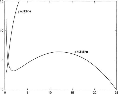
FIGURE 9.8 Nullclines for Equations 9.8.
We come now to the crucial point of our discussion. Even though xequil has been identified as an attractor, so all trajectories in its vicinity will eventually wind their way down to it; the path taken may vary enormously, depending on where the trajectory begins. The pivotal idea here is that two solutions that begin close together can have widely diverging orbits. One of them will make a large excursion before damping down to the equilibrium, and the other will barely move at all. This phenomenon is called excitability: As the model parameters r and k vary, there is a threshold for these values below which a solution to the equations will remain relatively quiescent but will suddenly blossom into a large orbit when the threshold is exceeded. In biological terms we think of the system as inhibited in one case and activated in the other, not unlike the blood clotting model of Section 9.7.
In Figure 9.9 two trajectories are plotted that begin nearby. We imagine that a small shock has perturbed the parameter values in such a way that the solution begins at the slightly displaced location shown in the figure. This position is below the x-nullcline, and so the ensuing orbit will move to the right until it crosses over to above the nullcline and returns to the equilibrium. Thus, the trajectory damps down to the attractor in one instance and is excited into a large orbit in the other, which shows that exceeding a threshold can trigger a rapid proliferation in the values of x and y. This is an algal bloom.
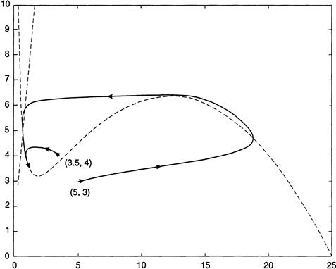
FIGURE 9.9 Trajectories for the Equations 9.8 for two nearby starting values of the variable x, with nullclines shown as dotted lines.
In terms of our model, excitability means that there is a rapid jump from a low endemic level of A.a., when this nuisance organism is merely a background species, to a surge in cell counts. After the bloom is initiated there is a refractory period during which high cell counts persist for a spell, even if the conditions that ignited the bloom have subsided. In terms of Figure 9.9, this means that once the trajectory has moved far enough to the right, a sudden change in a parameter value back to its subthreshold level will have little effect on the subsequent path followed by the trajectory; it will continue on a wide arc until it eventually declines rapidly toward the equilibrium. To put it another way, once the “die is cast,” there is enough inertia in the system to allow the bloom to sustain itself even if the triggering agents have, in the interim, fallen to subthreshold levels. In the Peconic estuary, for example, increases in the temperature and salinity of the water, which have the effect of raising the values of r and k, are implicated as factors that elevate cell counts of A.a. If a threshold is exceeded and a bloom ignited, then, as the high cell counts progress through weeks and even months into the late summer, it will often happen that both temperature and salinity have already waned. The protracted nature of the algal outbreak appears to be a manifestation of the refractory behavior exhibited by the model.
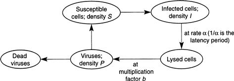
9.6 Viral Contamination of Algae
There is a body of evidence suggesting that the sudden demise of an algal bloom of the type described in the previous section is due to viral contamination. When algae cells reach high concentrations during an episode of profligate growth, it becomes easier for a virus to infect the cells by penetrating the membrane wall, from where it replicates itself until the cell bursts (cell lysis), releasing a multitude of new viruses that can then infect healthy cells in the surrounding medium. If the cell concentration is sparse, it is more difficult for a virus to find a nearby host cell. A simple model of this phenomenon follows considerations quite similar to the epidemic model of Section 9.2. The algae cells are divided into classes of susceptible and infected, with concentrations indicated by S and I, respectively, whereas the viruses have concentrations P, and these quantities interact as in the schematic of Figure 9.10. The irreversibly damaged infected cells contribute to cell density even though they do not reproduce, and collectively the cells have a maximum population density K, according to a logistic law, with a constant per capita rate r. The healthy cells become infected at a rate k proportional to the number of encounters between these cells and the viruses, and the viruses are depleted at the same rate. The infected cells are lysed at a constant per capita rate α (the reciprocal of this rate is the latency period, as in the model of Section 9.2), while the viruses reproduce at a rate that is some multiple b of the depletion rate of infected cells (b is generally of the order of tens to hundreds). The viruses die off at some constant rate μ that depends on a number of hostile factors in the waters. Putting all this together gives rise to the following differential equations:
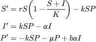
After a certain amount of algebraic juggling, the equilibrium solutions to this trio of equations become
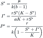
Evidently a feasible (non-negative) solution requires that b > 1. As b increases beyond this value, S∗ decreases until it is finally no greater than K, as it must be since this is the carrying capacity of the population of cells. It is readily established that this occurs when b achieves the value b = 1 + μ/kK. For any value of b ≤ b, the replication factor is too small to support a viral invasion of the algae cells.
Now consider the virus-free equilibrium (S, I, P) = (K, 0, 0). The Jacobean matrix of the linearized system at this equilibrium is given by
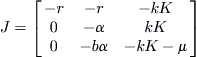
This leads to a cubic characteristic polynomial
![]()
whose roots are the eigenvalues of J. One root is immediately seen to be real and negative, namely, λ1 = – r. Solving for λ in the other quadratic factor and using the fact that S∗ = μ/k(b – 1) and assuming that b > b, we get two real solutions λ2,3, one of which is negative and the other positive. Therefore the equilibrium is unstable, thereby signaling the onset of a viral contamination, which now becomes endemic. In the paper by Beretta and Kuang [16] it is established that when S∗ is small enough, the conditions are propitious for a Hopf bifurcation, leading to oscillatory behavior. However, this consequence of the model equations would be difficult to observe in a turbulent ocean environment. What is noteworthy is that when the replication parameter b is greater than a certain threshold, it becomes possible for viral contamination to initiate the disintegration of the algal bloom.
9.7 Blood Clotting
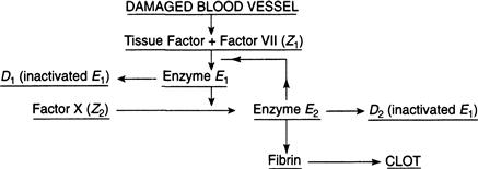
Running up stairs, a boy trips and scrapes his knee. Blood begins to ooze from the lesion, but not for long. The broken blood vessels have released something called tissue factor (TF) that reacts with a protein in the bloodstream to form a complex that we call Z1. This begins a chain of reactions that ultimately leads to the formation of fibrin, a protein that is polymerized into the gelatinous clump that we know as a blood clot.
The initiation of this blood-clotting cascade of biochemical interactions first requires that Z1 be converted into an active form before it can be useful. This occurs by means of an enzyme E2 that cleaves Z1 into its activated form. The letter Z stands for zymogen, an enzyme precursor, and the activated form of Z1 is another enzyme that we call E1. This enzyme then interacts with yet another protein, Z2, in the bloodstream, also known as factor X, to form the very same enzyme E2 that initiated these reactions in the first place, and, by so doing, it stimulates its own production. E2 then goes on to interact with other blood proteins besides Z1 until the full set of reactions has reached completion.
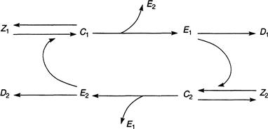
This self-enhancing loop of reactions, a chain of positive feedbacks, is illustrated in Figure 9.11. The production of E2 is bootstrapped by stimulating the formation of E1 from a supply of Z1, which, in turn, activates a supply of Z2 to form even more E2. The ability of E2 to catalyze its own formation ensures that a large supply of clotting proteins is rapidly produced. However, to safeguard against an overzealous production of clots, both E1 and E2 are quickly inhibited, either by binding with other blood proteins called inhibitors or by a process of negative feedback in which E2 acts indirectly to inactivate E1 and, therefore, itself. The inactivated products are denoted by D1 and D2 in the schematic of Figure 9.11. The delicate interplay between activation and inhibition results in an initial burst of clotting followed by a rapid decline in the levels of all the enzymes involved in coagulation. This leads to what is in effect a system “shutdown” when the job is done.
The needed proteins are in plentiful supply in the blood plasma, and clotting will initiate whenever they are activated. We can get a bit colloquial here and say that the clotting system is “idling” prior to an injury. There is a threshold below which the clotting cascade is not triggered into action, since small-enough tissue damage should not result in large clot formation because vagrant clots can lead to a fatal thrombosis. After all, blood vessels are being ruptured every time we knock against something, however slightly, and an all-out response is generally unwarranted. By the same token, once the threshold is exceeded, the system must be stimulated into action to avoid bleeding to death.
Our goal is to write down differential equations to model the reactions that represent the initial phase of clotting and to derive from this the threshold condition for system activation. We begin first by looking at the simplest case, in which a single enzyme E catalyzes its own formation without requiring the intervention of other enzymes, a situation that actually arises in certain biochemical reactions and is known as autocatalysis. E combines with a protein Z (in enzyme kinetics Z is called a substrate of E) to form a complex C. This is a reversible reaction that occurs at a rate proportional to the concentrations of E and Z, with a rate constant k+, and that can then dissociate back into its constituents at a rate proportional to the concentration of C itself, with rate constant k−. When the reaction energy is high enough, E will cleave Z to form more E at a rate k, proportional to the concentration of C. E is then inactivated into form D (for “dead”) at a rate proportional to its own concentration, at rate k1. This feedback loop, shown in Figure 9.12, gives rise to two differential equations:
![]() (9.9)
(9.9)
There is an initial amount of Z, namely, Z0, which diminishes as the reaction progresses, but the amount of E can vary up or down. At any instant of time either E and Z are freely available or they are bound up in the complex C. However, their total amounts are conserved, and so we have the relations
![]() (9.10)
(9.10)
If we substitute (9.10) into (9.9), the right-hand side of the first equation becomes a quadratic in C with roots r1 and r2 that are real and positive. Let’s assume that r1 > r2. Then the first equation in (9.9) can be written in terms of its factors as
![]() (9.11)
(9.11)
If one assumes that Z0 is in large excess over the initial concentration of E during the initial phase of the reaction, which is usually the case, then the binding of E to C will take place rapidly, or, to put it another way, the change in Z is “slow” as compared to the “fast” formation of C. C moves quickly to the attractor r1, where it assumes its equilibrium value. To verify all this, note that after inserting relations (9.10) into the equation for C in (9.9), you obtain C′ = C2 – (Z0 + ET + km)C + ETZ0 = (C – r1)(C – r2), where r1 and r2 are the two roots of the quadratic right-hand side of the equation for C. A straightforward computation shows that these roots are real and positive. Using the method of separating variables, the equations can be expressed as ∫ dC/(C – r1)(C – r2) = ∫ dt, and this can be integrated to yield log[(C – r1)/(C – r2)] = log r + (r1 – r2)t, where r is r1/r2. Solving, we obtain ![]() . After a negligibly brief period, therefore, C is essentially equal to the constant obtained by setting C′ to zero:
. After a negligibly brief period, therefore, C is essentially equal to the constant obtained by setting C′ to zero:
![]()
where ![]()
Because C rapidly adjusts to any initial value of Z, we may as well replace Z0 by Z itself, whatever its value happens to be initially. Also, the clumsy Etotal is now replaced simply by E, with the understanding that E stands for the total (and time-varying) amount of enzyme present in the reaction. With this convention, the preceding expression for E becomes, after some simple algebra,
![]() (9.12)
(9.12)
Relation (9.12) is known as the Michaelis–Menten equation.
The protein Z is consumed at the same rate that E is produced, and so there is an additional equation to consider:
![]() (9.13)
(9.13)
with the minus sign indicating that Z is decreasing. Some progress can be made toward solving the equation pair (9.12) and (9.13) if we notice that since Z changes very little, at least during the initial phase of the reaction, Km is considerably greater than any change in Z that takes place. Because of this, Km + Z is essentially constant, and so the equations become
![]() (9.14)
(9.14)
with a = k/(Km + Z). A nullcline approach now shows that E is activated (that is, it will increase in value before eventually decaying to the attractor zero) whenever Z exceeds k1/a. Otherwise E goes quickly to zero. Rather than pursue the consequences of this, let us return to the original problem, in which there are two enzymes E1 and E2.
To derive the appropriate differential equations it suffices to mimic the argument used earlier. To begin with, E2 and Z1 combine to form a complex C1 as a reversible reaction that occurs at a rate proportional to the individual concentrations of E2 and Z1, with a rate constant k+, and it dissociates back into its constituents, with a rate constant k−. When the reaction energy is high enough, E2 will cleave Z1 to form E1 at a rate m1. Then, after the cleavage is complete, E2 is released and becomes available again. A completely parallel set of reactions leads to a complex C2 from the combination of E1 with Z2. This is illustrated in the schematic of Figure 9.13.
We are led, as before, to an equation for the formation of C1:
![]()
The product of this reaction, E1, follows the equation
![]()
in which we assume that E1 is inactivated to D1 at a rate proportional to its own concentration, with proportionality constant k1.
At any instant, the enzyme E2 either is available in free form or is bound up in the complex C1. It follows that
![]()
where T stands for “total.”
At this juncture we observe that during the initial stage of coagulation, Z1 and Z2 are in large excess over E1 and E2 before any substantial conversion of these blood proteins has taken place. As in the simpler case of a single enzyme, treated earlier, this ensures that the binding of E2 to Z1 (and, similarly, of E1 to Z2) takes place rapidly. Thus C1 very quickly reaches a nearly constant saturation value, whereas Z1 remains essentially constant as some value Z10. This enables us to assume that C1 is at a stable equilibrium in which its derivative is zero. Combining this with (9.12) and (9.13) results in
![]()
where ![]() stands for the ratio (m1 + k−)/k+. Because C1 quickly adjusts to any initial value of Z1 we repeat what was done earlier and replace Z10 by Z1 itself, whatever its value happens to be initially. From Equation (9.13) it now follows that
stands for the ratio (m1 + k−)/k+. Because C1 quickly adjusts to any initial value of Z1 we repeat what was done earlier and replace Z10 by Z1 itself, whatever its value happens to be initially. From Equation (9.13) it now follows that
![]() (9.15)
(9.15)
in which E2T is replaced simply by E2, with the understanding that E2 denotes the total amount of this enzyme, with a completely analogous meaning for E1. We therefore have a similar equation for E2, obtained in an identical manner:
![]() (9.16)
(9.16)
Since Z1 and Z2 are consumed at the same rate as E1 and E2 are produced, it is also true that
![]() (9.17)
(9.17)
![]() (9.18)
(9.18)
Equations (9.15) through (9.18) can be linearized about the equilibrium values, in which Z1 and Z2 are assumed constant at some values Z10 and Z20 and where E1 and E2 are zero. This leads to two linear equations:
![]() (9.19)
(9.19)
Here, the constants ![]() are composites of the several constants appearing in the previous equations. The behavior of this system depends on the eigenvalues of the matrix
are composites of the several constants appearing in the previous equations. The behavior of this system depends on the eigenvalues of the matrix
![]()
because this tells us whether the equilibrium at the origin of the E1, E2 plane is an attractor or not. If it is, then any initial value of the enzymes will decay to zero, and the system remains subthreshold, whereas an unstable equilibrium implies an explosive growth in these enzymes, signaling an initial catapulting in the amounts produced. This is the above-threshold condition that leads to clot formation. Of course, the linear equations cannot tell us what happens far from equilibrium after the initial onset of activity. For this, one needs to integrate the full set of nonlinear equations and see how the system evolves over time. First, however, let us find the threshold condition by checking the eigenvalues. A quick computation based on A above shows that if θ > 1, where θ = a1a2/k1k2, the equilibrium is unstable (one eigenvalue is positive, the other negative). This is because the trace and determinant of the matrix A are both negative. Otherwise, with θ < 1, the equilibrium is an attractor with two real and negative eigenvalues since the determinant is now positive. Note that θ is a quotient of activation to inhibition rates, and it is this ratio that determines whether the clotting system will ignite or not. A large-enough injury will release a sufficiently large amount of tissue factor, and coagulation then gets off the ground by guaranteeing that θ will exceed unity. If the inhibition rates ki are large enough, for example, then no clotting will take place. Patients with severe clotting problems are sometimes treated with an infusion of the anticoagulant drug heparin that actually increases these rates. The oral “blood thinning” drug warfarin, taken by heart-attack victims, achieves similar results by decreasing the constants mi.
An integration of Equations (9.15) to (9.18) is shown in Figure 9.14, in which there is initially a small amount of E1 present to get the process started. The two plots show E1 under sub- and above-threshold conditions. In the first instance, E1 decays to zero; in the second we see a substantial rise in its concentration as a result of activation, but with an eventual decay to zero again because of inhibition.
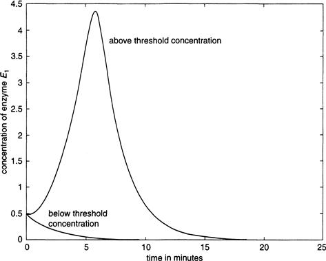
FIGURE 9.14 Threshold response for the activation of enzyme E1, from the blood clot model Equations (9.15) through (9.18).
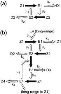
But there is more to the story of clotting. It is a complex system. Let’s redraw Figure 9.13 in a more schematic form as Figure 9.15a and beside it, in Figure 9.15b, an extension of the feedback cascade of reactions to include two new enzymes E3 and E4 that catalyze their own formation after being activated by E2. The point I wish to focus on here is not these short-range reactions but, rather, the long-range activation loop from E4 to generate more E1 from Z1. This positive feedback loop allows the system to bootstrap itself, as will be seen. Without going into details, the linearized equations that correspond to this extended chain of reactions, obtained by perturbing about an initial equilibrium state in which Ei are all zero and Zi, i = 1, 2, 3, 4, are at their nonzero starting values, Zi = Zi0 can be written as a quartet of equations. Then (see the original reference cited in Section 9.8) the characteristic polynomial of the 4 × 4 Jacobean matrix at the equilibrium is given by a quartic equation,
![]()
where a = m1m2Z10Z20, b = m3m4Z30Z40, and C is the constant m1m2m3m4m5Z10Z20Z30Z40.
The case of no long-range feedback occurs when C = 0, since this is the only term that includes m5. Each factor in f(λ) = 0 is precisely of the same form as in the previous, single-loop situation. Therefore, the double loop is activated if the threshold condition θ > 1 is valid or if a similar condition holds for the second loop, namely,
![]()
Suppose now that in the absence of the long-range feedback loop (C = 0), we have θ1 < 1 and θ2 < 1. This means that f(λ) = 0 has all its roots both real and in the left half complex plane, and so the equilibrium is stable, which implies that no clotting cascade will initiate. What choice of positive constants a, b, k1, k2, k3, k4 (which depend on the level of activation and inhibition) do we need to destabilize the system?
When the feedback term is included, the characteristic polynomial becomes f(λ) – C, where C is a positive constant that depends on the feedback, as already noted. When C = 0, one sees that f(λ) → ∞ as |λ|→ ∞ and f(λ) has the form displayed in Figure 9.16. When C > 0, the effect is to shift the graph of f(λ) downward until, at some specific C value, one obtains the graph that is also shown in Figure 9.16. Beyond this threshold there is a positive root, and the system is now unstable, as required. The remaining roots are real and negative, or there are two complex conjugate roots together with one negative real. At this juncture one has the conditions necessary for a clotting cascade to progress.
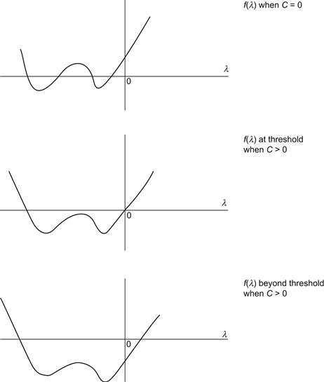
FIGURE 9.16 Plots of the fourth-order characteristic polynomial f(λ) – C = 0 for three values of C.
The case C = 0 represents the absence of long-range feedback.
As we have attempted to emphasize in this chapter, clotting is characteristic of a wide class of living systems that exhibit excitability in response to a large-enough stimulus.
Note that if one differentiates the first-order linear equations (9.19) for E1 and E2, one then obtains a single second-order differential equation. In fact E′1 = a1E2 – k1E1 yields E″1 = a1(a2E1 – k2E2) – k1E′1. But a1E2 = E′1 + k1E1, from which we find that E″1 = (a1a2 – k1k2)E1 – (k1 + k2)E′1. Now let u = E′1/E1. Then a simple computation shows that u′ = –u2 – (k1 + k2)u – (k1k2 – a1a2). This first-order equation in u is known as a Riccati equation. Setting the right side of the equation to zero gives us the two equilibrium points, namely, λ1, λ2 = –(k1 + k2)/2 ± [(k1 – k2)2/4 + a1a2)]1/2. To obtain one positive and one negative root, as required for instability, it is necessary that θ = a1a2/k1k2 > 1, replicating the condition obtained earlier.
9.8 Concluding Thoughts
Equations (9.6) can be simplified further by ignoring the birth rate r. This supposes that the population size is fixed, with no new recruits or defections during the period of an epidemic, which is a reasonable assumption for diseases of short duration. The equations now read as
![]() (9.20)
(9.20)
The fraction R of recovered individuals is initially zero, and, because S + I + R = 1, this means that S + I = 0 at t = 0. From the chain rule of differentiation one obtains, for all S, I in the positive quadrant,
![]()
Integrating both sides of this relation with respect to S yields
![]() (9.21)
(9.21)
Assume that c/b < 1. Plot the solution curves in the S, I plane, and interpret the results in light of the discussion in Section 9.2. Show, in particular, that if S is initially greater than c/b, there is an epidemic, after some infectives are introduced into the population, whereas if S begins at some value less than c/b, the disease doesn’t take root and the infectives diminish over time. This is the threshold condition. In any case, show that the epidemic dies out, not for any lack of susceptibles in the population, but, rather, because there are no more infectives.
Note that Equation pair (9.20) is formally equivalent to the model Equations (9.14) for autocatalysis in blood clotting. Indeed, both models observe a threshold condition for growth and decay, suggesting similarities in the underlying dynamics.
After the vaccination of schoolchildren began in earnest in many communities around 1963, the incidence of measles declined significantly, only to reappear among preschoolers during the late 1980s (see, for example, “Resurgence of Measles Prompts New Recommendations on Vaccination,” New York Times, Jan. 11, 1990). The idea that some recurrent epidemics are a manifestation of chaotic dynamics is based on the paper by Olsen and Schaeffer [95] and is reviewed in a short note by Pool in Science [97]. An elementary introduction to chaotic attractors is to be found in the Scientific American article by Crutchfield and others [39]. Epidemic models are given a comprehensive treatment in the Anderson and May book [3].
The discussion of Section 9.6 is taken from Beretta and Kuang [16], who, in turn, acknowledge that the model is due to some unpublished lecture of Akira Okubo. Their work considers marine bacteria instead of algal cells, but the results extend to this case as well (in this regard see Milligan and Cosper [83] and also Nagasaki et al. [89]). An interesting article on this topic by Marks is from the New York Times, Nov. 4, 1994, “Natural Virus Said to Check Brown Tides.”
The model of Section 9.5 is taken from Beltrami [11], while the model of predator-mediated coexistence of Section 9.4 is based on a short note by Gilpin [53].
The threshold condition for blood clot initiation that was discussed in Section 9.7 is from the paper by Beltrami and Jesty [13]. It is worth mentioning here that there is a spatial version of this model that accounts for the size of an injury on the initiating of a clotting cascade (Beltrami and Jesty [12]) that is a prequel to the spatial models to be considered in the next chapter involving the combination of reaction terms and spatial diffusion. We do not give details of this clotting model here since they involve several biochemical technicalities. Suffice to say, the results are not very different in kind from those of Section 10.2.