
Boom and Bust
8.1 Background
In his novel Cannery Row John Steinbeck vividly describes the bustle of a sardine factory in Monterey, California, before the Second World War, when heavily laden boats brought in the abundant catch of the sea. But the industry suffered a sharp decline as the sardine population collapsed in the late 1940s and the once-thriving canneries began to close down. Later, in the early 1970s, a similarly precipitous drop in the catch of anchovies occurred in Peru, then the largest fishery in the world. What happened? Although some episodic shift in climate may have had an influence, especially the influx of warm waters known as “El Niño,” which occurs sporadically off the Peruvian coast, the dominant factor in each instance was, quite simply, overfishing.
When commercial fishing begins along some coastal region, this sets in motion an investment in fishing gear that continues to increase to exploit what initially appears to be an ample natural resource; within a few years, a sizable fleet plies the waters. As fish stocks dwindle and prices rise, the competition among fishermen intensifies, and even more aggressive fishing tactics may be the response. Certain species of fish, such as sardines, anchovies, and herring, swim in schools that not only favor their detection and bulk harvest but, in biological terms, may diminish their ability to breed due to low population densities. This implies that an overly exploited species can have a diminished capacity to recruit new adults. In Section 8.2 a model is presented that combines both economic and biological considerations and that exhibits how the sudden collapse of just such a species becomes possible as a critical level of harvesting is reached.
Since the model is but the first that involves nonlinear differential equations, I undertake a brief review of the salient facts about such equations in Section 8.3, leaving more technical details to Appendix C and the reference mentioned in the final section.
The stimulus to changes in the natural world are not always sporadic and unpredictable. Cyclic or nearly cyclic phenomena abound in nature as biological systems respond to periodic fluctuations in the environment around them. One thinks of daily rhythms that are “tuned in” to night following day following night or of bodily rhythms as well as insect and plant behavior that are influenced by lunar and seasonal cycles. Periodic orbits can also come about from the interplay between activation and inhibition. In the fish-harvesting model, for example, the self-enhancing growth of fish is balanced by exploitation, which gives rise to cyclic behavior, as we will see in Section 8.4, where we take a second and quite different look at the model.
Finally, in Section 8.5, we consider two competing fishing fleets plying the same waters. Each wants to maximize its return as both exploit a common resource, but each is hindered by the presence of the other. We will think of this as a game fed by mutual distrust and greed.
8.2 A Fishery Model
It appears that sardines and similar species of fish have a difficult time breeding at low population densities, and their survival is enhanced with increasing density, up to a level at which overcrowding begins to have an inhibitory effect on reproduction. This is achieved by swimming in “schools,” large and closely packed swarms, because this confers more protection from predators. Unlike some other species, which follow a logistic per capita growth rate r(1 – x/K), which decreases linearly with an increase in density x, the per capita growth rate of sardines is probably better modeled by a term that begins low and increases with x for a while before decreasing. This would reflect an initially low growth rate that increases with population density x and then declines when x is large. A simple example of this is the function rx(1 – x/k).
Consider now a fishing zone with unrestricted access. Any number of fishermen, with their trawlers and nets and, in recent years, electronic fish detectors, can harvest the fish. Let E be the total fishing effort in terms of the vessels and fishing gear as well as manpower deployed per unit time, and let v denote the fraction of each ton of fish that is caught per unit effort. Then vEx is the total catch per unit time, where x is the fish density in the fixed zone, measured in tons. An increase in E signifies that fishing effort has intensified. If we adopt the per capita reproduction rate of schooling fish, then the rate of change of x is given by the differential equation
![]() (8.1)
(8.1)
where the second term on the right reflects the loss due to fishing and the superscript prime indicates differentiation with respect to time.
Now we introduce some drastically simplified market economics. Suppose that the cost, in dollars, per unit effort is c and that p is the price obtained for the fish at the pier, in dollars per unit catch. The cost includes operating expenses as well as an amortized capital investment, while p reflects the market value of the fish. The net revenue from the harvest is proportional to pvEx – cE. As long as this quantity is positive, the fishing effort increases. This follows from the idea that when a natural resource has unrestricted access, its exploitation continues unabated until the resource no longer provides any profit. In the case of a fishery the harvesting would increase until the net revenue is zero or until the existing fish stock is exhausted. A fisherman who does not participate in the haul relinquishes his portion of the take to his competitors. A sole owner of the fishery might want to harvest less relentlessly, because a prematurely depleted fishery does him no good, and he has the incentive to balance a short-term gain from aggressive fishing against the potential long-term benefits of gradual exploitation. But in an open-access fishery, the short-term myopic view prevails that as long as a profit is to be made there is no reason to incur a loss by not joining the scramble for what is left.
Of course, this is a gross simplification because no fishery is totally unregulated, and, as fish stocks begin to be depleted, a conservationist attitude becomes more prevalent among the regulating agencies. Moreover, as competition intensifies for a dwindling resource, the effort must necessarily increase, which would discourage those fishermen who have alternative employment opportunities. Nevertheless we adopt this somewhat fictional view and write an equation for the rate of change of fishing effort as another differential equation:
![]() (8.2)
(8.2)
This equation tells us that E increases or decreases at a rate proportional to the net revenue with a constant of proportionality α. If the net profit is positive, it increases; otherwise it decreases. This constant of proportionality is generally small, to reflect the fact that there is a certain inertia in the way the fishing industry responds to a perceived change in either market conditions or the availability of fish in the ocean. It takes some time to hire or lay off personnel, invest in new gear, or to put additional boats out to sea. These changes take place at a slower pace than the breeding of fish. For this reason, E is considered to be a slow variable relative to x, which is deemed to be fast.
At this juncture we need to modify Equation (8.1) by adjoining a small constant e:
![]() (8.3)
(8.3)
The interpretation of the constant e is that even when the observable population density x is zero, some additional fish are spawned, because a few members of the species found a refuge or because additional fish migrate into the fishing zone at some constant rate. We are considering a threshold effect here that just barely allows for the possibility of recovery. It also embodies the idea that when fish stocks are sufficiently reduced, further exploitation ceases, either because it isn’t worth the effort or because a regulatory agency has imposed a ban.
Our fishery model consists of the coupled Equations (8.2) and (8.3).
We begin the discussion by noting that the scalar Equation (8.3) has either one or three equilibria, depending on the values of E, which are obtained by setting x′ to zero. This occurs at the intersection of the curve g(x)/vx with the line defined by E = constant, in the x, E plane, where g(x) = e + rx2(1 – x/K). This is illustrated in the six panels of Figure 8.1 for different values of E.
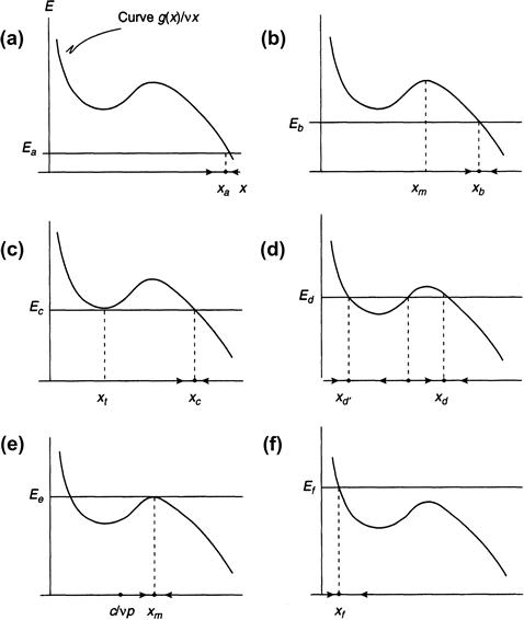
FIGURE 8.1 The curves g(x)/vx and E = constant, for six different values of E, showing the equilibrium values of the fish stock x as obtained from model Equation (8.3).
E is treated as a slowly changing parameter relative to the fast variable x, and the six panels are snapshots of how fish stocks change in response to changing values of harvesting rates.
By examining the sign of x′ we can determine the stability properties of the equilibria, as is explained in more detail in the subsequent section. A single equilibrium is always an attractor; but if one has three equilibria, the middle one is always unstable (if these terms are not clear, please consult the next section before continuing). This follows from the fact that x increases or decreases according to whether the value of E is less or greater than g(x)/vx.
Because E varies slowly with respect to x (recall that α is a small constant), it follows that x responds quickly to a change in E and so it resides at or near its closest attractor. This means that a study of the pair of equations for x and E can be simplified considerably by letting E be a gradually changing parameter in the single Equation (8.3) for x. The fish level then corresponds to the value of x that occurs at the intersection of E with g(x)/vx.
Consider now the following scenario. Initially the fishing effort is slight, say, Ea, and so a single equilibrium occurs at a high value of x, indicated by xa in Figure 8.1a. This is an attractor, as we already noted, and so the fish stock is xa when fishing effort is Ea. A modest increase in E to Eb reduces the equilibrium to xb, but, even though fish density x is now less, the total yield vEx is greater (Figure 8.1b). To see why this is so, observe that the function g(x)/vx achieves its local maximum at the hump shown in Figure 8.1b at the point xm. The derivative of this function is therefore zero there, and its second derivative is negative. It can be shown, in fact (the computational details are shown later, in Section 8.5), that g(x)/x = g′(x) at xm. Now the yield, namely, the function h(x) = vEx, is a straight line that intersects the function g(x), and, as shown in Figure 8.2, the value of h(x) at the point of intersection at the point xm is where g(x)/x and, therefore, the yield attains its maximum. The corresponding value of E, namely, Em, is called the maximum sustainable yield. Until E reaches the value Em, the yield continues to increase.
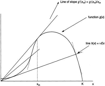
FIGURE 8.2 Intersection of the curve g(x) and the straight line h(x) = vEx for different values of E.
As E increases beyond Eb, there is a value Et at which the line E = constant is first tangent to the curve g(x)/vx (Figure 8.1c). The point of tangency occurs at x = xt and is called a bifurcation point, since two new equilibria are created for all E that are just beyond this point of tangency. However, the equilibrium at xc is still an attractor. There are three equilibria when E = Ed, as can be seen in Figure 8.1d, but the middle one is unstable, and, because x moves quickly to the nearest attractor, the fish density resides at xd and does not move to the other attractor at xd.
Beyond this level of harvesting effort, the fish stocks continue to decline and prices begin to rise through scarcity. Ironically this can draw new entrants into the fishery, and the competition to catch intensifies as long as c/vp is less than xm, where ![]() attains its local maximum, since this implies that the derivative E′ in Equation (8.2) remains positive. As E increases beyond Ed, we enter a phase of biological overfishing, since immature fish begin to be captured before they can breed; eventually, when the point of tangency at xm is attained, there is another bifurcation, at which two of the equilibria coalesce and disappear (Figure 8.1e), beyond which there is a single equilibrium at a much lower fish density xf, where E = Ef. This is an attractor, so the fish stocks suddenly fall to this new equilibrium, an event that signifies the collapse of the fishery (Figure 8.1f).
attains its local maximum, since this implies that the derivative E′ in Equation (8.2) remains positive. As E increases beyond Ed, we enter a phase of biological overfishing, since immature fish begin to be captured before they can breed; eventually, when the point of tangency at xm is attained, there is another bifurcation, at which two of the equilibria coalesce and disappear (Figure 8.1e), beyond which there is a single equilibrium at a much lower fish density xf, where E = Ef. This is an attractor, so the fish stocks suddenly fall to this new equilibrium, an event that signifies the collapse of the fishery (Figure 8.1f).
Assume now that the ratio c/vp is greater than xf. We see from Equation (8.2) that the derivative E′ is now negative, and so fishing effort reverses itself. In effect it no longer pays to go out to sea, and many trawlers begin to rust in the harbor.
Eventually recovery of the fish stocks takes place because of reduced harvesting. As E decreases, the situation pictured in Figure 8.1d eventually reappears, but now the fish density moves to its nearest attractor, namely, xd′. By reducing E further, there is ultimately only one attractor, at the relatively high value just beyond xc (Figure 8.1c). The fish density therefore makes a sudden resurgence at a level that exceeds c/vp, where the derivative of E is once again positive. We assume here that c/vp is between xt and xm; otherwise, for c/vp less than xt, fish recovery is less dramatic than indicated in the present scenario.
Some ships feel encouraged to go out to sea, and the process starts over again, leading to a cyclic boom-and-bust population dynamic. A hysteresis effect takes place in which the path to recovery follows a different route than the path to collapse (Figure 8.3). A more complete discussion of this cyclic behavior is reserved for Section 8.4.
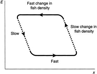
FIGURE 8.3 Stable equilibrium values of the variable x in response to changes in E.
As fishing effort E increases and then decreases, a hysteresis effect is observed in which fish density x follows a different path from collapse to recovery.
We have attributed a crash in fish density to overfishing. There could also be unfavorable climatic changes that restrict the rate at which fish larvae develop into young adults. This corresponds to a decrease in the rate constant r. These are called recruitment failures, and an already seriously depleted fishery is especially prone to collapse when an environmental fluctuation such as “El Niño” occurs. Moreover, a diminished species can be replaced by other, commercially uninteresting species, and these may inhibit the recovery of the original fishery. In the preceding section we saw how this can happen when one of two strongly competing species drives the other to extinction as we move from one basin of attraction to another.
The present model assumes there is no seasonal preference for hatching and that reproduction is unaffected by age and sex differences. In spite of these and similar simplifications, the model appears to mimic the gross behavior of certain types of fisheries, such as anchovies and sardines, in which excessive exploitation can lead to a sudden collapse followed by gradual recovery.
A dramatic example of such a collapse is provided by the Peruvian anchovy fishery. Using the number of vessels deployed per unit time as a measure of effort, the actual catch (in 106 tons) was given by
| Year | Effort | Yield |
| 1959 | 1.4 | 1.91 |
| 1964 | 5.8 | 8.86 |
| 1968 | 8.9 | 10.26 |
| 1973 | 46.5 | 1.78 |
As E increased from 1963, so did the catch. But by 1973 the yield had fallen to pre-1959 levels.
If the cost-to-price ratio c/p increases to a level at which c/vp exceeds xm, the fishery avoids a crash, as can easily be checked from Equation (8.3). This can be ensured by governmental intervention in the form of imposing a tax T per unit catch. This effectively reduces the net price for the fish to p – T; if the tax is severe enough, c/v(p – T) will indeed exceed xm. There are other regulations that can be and are imposed on fisheries, especially after a disastrous failure, such as catch quotas, licenses and fees that restrict the entry of additional fishermen, and no-fishing zones. These are not considered here.
8.3 Unstable Equilibria and Cyclic Behavior
Because all the models in this chapter involve differential equations, we need to discuss some of the properties of simultaneous first-order ordinary differential equations in k dependent variables xi(t), 1 ≤ i ≤ k. The xi define the states of a dynamical system in terms of an independent variable t that is regarded as time:
![]() (8.4)
(8.4)
The superscript prime denotes differentiation with respect to t (we suppress, for notational convenience, the explicit dependence on t in this and subsequent chapters), and the fi are generally nonlinear functions of the k variables. Vectors are columns of real numbers, but for typographical convenience I represent them as transposes of row vectors. With this in mind, define
![]()
and
![]()
A compact version of (8.4) can now be written as
![]() (8.5)
(8.5)
The vector x(t) defines the state of the dynamical system at any time t, and it traces out a solution curve in k-dimensional space, called a trajectory or an orbit, that describes how the system moves in time.
We assume that the equations are an adequate representation of an observable process, and so, on purely intuitive grounds, it is reasonable to expect that the equations have solutions that mimic the actual time evolution of the process itself. Specifically we assume that if the state is prescribed to have a value x0 at some initial time t = 0, then there is a unique vector valued function x(t) defined for all times t that passes through x0 at t = 0. Precise conditions on the vector function f can be given that guarantee that a unique solution with these properties does indeed exist, but we forgo the details because we already believe that the equations are well posed in terms of the processes that they describe. Any good book on the elementary theory of differential equations can be used to fill in the mathematical details that are sidestepped here; the book by Hirsch, Smale, and Devaney [62] is especially recommended (see also Appendix C for additional details).
The uniqueness requirement is especially significant because it tells us that the time evolution of a dynamical system along individual trajectories follows distinct paths; if two trajectories were to cross each other, then their point of contact is an initial state from which two separate solutions emerge, a violation of uniqueness.
Some solutions remain constant in time. These states of rest, called equilibrium solutions, are defined by positions for which the time derivative x′ is zero. At an equilibrium, no motion ensues. Our concern is with knowing what happens to a trajectory as time passes. An equilibrium state x, called an attractor, is said to be asymptotically stable if all trajectories that begin in some sufficiently small neighborhood of x approach this equilibrium arbitrarily close as t increases. More specifically, there is a set Ω of initial states x0 such that the solution through x0 will lie in an arbitrarily small neighborhood of x when t is large enough. The largest set Ω for which this is true is called the basin of attraction. If no such bounded neighborhood exists, then x is considered unstable. An unstable equilibrium repels at least one trajectory in its neighborhood.
There are attractors other than equilibria. Trajectories that begin in some set Ω of initial states may, for example, tend toward a closed orbit that represents a periodic solution of the differential equations. An illustration of this is provided by the Van der Pol equation y ″ = –y + y′ (1 – y2), which becomes a first-order system
![]()
when we let x1 = y and x2 = y′.
The solutions in x1, x2 space are plotted in Figure 8.4. There is a single equilibrium state at the origin that is unstable because it repels all trajectories in its neighborhood. These trajectories spiral outward to the cyclic trajectory, whereas all solutions that begin outside the closed orbit eventually wind down toward it.
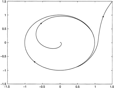
FIGURE 8.4 Integration of the model Equations (8.9) showing trajectories that spiral out to a periodic attractor.
There are other, more complicated, examples of attractors to be discussed later, but for now our attention will be confined to asymptotically stable equilibria, for which I quote a basic result whose proof can be found in the aforementioned reference [62]. The idea is to determine whether an equilibrium is attracting is based on the idea of approximating the system of nonlinear equations x′ = f(x) by a system of linear differential equations u′ = Au for some suitable matrix A. We have the following theorem.
We now discuss a theorem that tells us when cyclic attractors may be expected, at least for planar systems of two variables. This is called the Hopf bifurcation theorem, whose proof is sketched in Appendix C.
As before, we treat a system of differential equations whose solutions are vector-valued functions of time t, except that now we allow the dependency on some scalar parameter s:
![]() (8.6)
(8.6)
Our previous discussion has conditioned us to expect bifurcations to occur as the slowly varying s attains certain critical values. This will again be the case, but, in contrast to the bifurcations encountered earlier, we now seek periodic solutions.
Let xs denote an equilibrium solution to (8.6), in which the dependency on s is made explicit. The Jacobean matrix of the linearized equations will also depend on s, and we write the linearized system in vector form as
![]() (8.7)
(8.7)
It will be assumed that the eigenvalues λ of A(s) are complex:
![]() (8.8)
(8.8)
where the real and imaginary parts exhibit dependency on s as well. The following result is then valid under the usual conditions on differentiability.
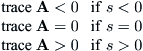
In view of Theorem 8.1, it suffices to assume that a(s) is negative (positive) when s is negative (positive) to ensure that xs is an attractor for s < 0 and a repeller for s > 0. However, that theorem tell us nothing about what happens when s = 0 because the real part of the eigenvalues is zero there. This is a delicate issue that needs to be resolved in each instance by referring to the nonlinear equations directly or, quite simply, by assuming that xs remains an attractor at s = 0 based on extraneous evidence supplied by our observations of the problem being modeled:
![]()
The determinant of this matrix is always positive, but the trace 2s can be of any sign. The eigenvalues are s + i and s – i, and so a(s) = s is zero at s = 0, whereas b(s) is the nonzero imaginary. The real part a(s) is simply trace/2, and its derivative with respect to s is 1. To see what happens when s = 0, make a change of variables in the equations by letting x = r(sin θz) and y = r(cos θz), where r represents radius in polar coordinates and θ is the angle. After a bit of algebra, the equations are transformed into the pair
![]() (8.9)
(8.9)
The second equation says that the angle is turning clockwise at a constant rate, whereas when s is zero, the scalar equation in r has an attractor at r = 0. In fact one can integrate r ′ = –r3 and find that r(t) tends to zero as t goes to infinity (assuming r(0) > 0). Thus the origin is in fact asymptotically stable for s ≤ 0, and so all the conditions of Theorem 8.2 are now satisfied. We conclude that there must be a periodic solution when s > 0. In fact an examination of the sign of the derivative r ′ in (8.9) immediately shows that when s > 0, the origin is a repeller while the circle of radius r = ![]() is an attractor. Hence the trajectories spiral outward from the origin toward the circle of radius
is an attractor. Hence the trajectories spiral outward from the origin toward the circle of radius ![]() and inward from positions beyond the circle. Moreover, the radius of this periodic attractor increases with s.
and inward from positions beyond the circle. Moreover, the radius of this periodic attractor increases with s.
8.4 A Second Look at the Fishery Model
An interesting application of Theorem 8.2 is to the fishery model of Section 8.2 because it leads to an alternate formulation of the “boom-and-bust” scenario that comes in the wake of overfishing. Referring to the discussion in that section, recall that the equations are written as
![]()
where g(x) = e + rx2(1 – x/K). Assuming that E > 0, the sole equilibrium occurs at x∗ = c/vp and E∗ = g(x∗)/x∗.
The quantity g(x)/x represents the per capita growth rate, and it has a maximum at some point xm (see Figure 8.1b). The derivative of g(x)/x at xm is therefore zero and so
![]()
at xm. This implies that
![]() (8.10)
(8.10)
Moreover, because g(x)/x is maximized at xm, its second derivative there is negative:
![]()
and, in view of (8.10), the last three terms cancel and we obtain
![]() (8.11)
(8.11)
The Jacobean matrix of the linearized equations corresponding to the nonlinear system for the variables x and E is readily computed at the equilibrium of this system and is
![]()
and we see that the determinant of A is always positive. To decide the sign of the trace g′(x∗) – g(x∗)/x∗, refer to Figure 8.2, where we see that where the line h(x) = vEx intersects the curve g(x), the slope of h(x) is g(x)/x. At x = xm, however, the slope of g(x) is identical to g(x)/x, as can be seen. If the intersection occurs at a point where x is less than xm, then the slope of the line is less than the slope of curve g; just the opposite is true when x exceeds xm (Figure 8.2).
Because of these considerations, the trace of the Jacobean of A, namely, g′(x∗) – g(x∗)/x∗, is positive when x∗ < xm, zero if x∗ = xm, and negative otherwise. Let s = xm – x∗ be a bifurcation parameter. Then
or, put in other terms, the equilibrium is an attractor for s < 0 and a repeller for s > 0. Because the determinant of A is positive, the discriminant of the quadratic equation that determines the eigenvalues will be negative when trace A is close to zero. Hence there is a range of s values, say, |s| < δ, for which the eigenvalues are complex. The fact that the determinant is nonvanishing also guarantees that the imaginary part of the eigenvalues is nonzero at s = 0, even though the real part is zero there.
Our previous analysis of the fishery problem revealed an up-and-down oscillation in the values of the fish stock x as the harvesting parameter E slowly varied (Figure 8.3). This suggests that we might expect a bifurcation to an attracting cycle to emerge when s exceeds zero. Thus, even though we have no direct evidence that the equilibrium is an attractor for s = 0, it is quite plausible that this is in fact the case.
To complete our analysis we need to establish that the derivative with respect to s of the real part of the eigenvalues, namely, the derivative of (trace A)/2, is positive at s = 0. Now, x∗ = xm – s, and therefore, by utilizing the chain rule of differentiation one computes this derivative to be
![]()
and the second two terms within braces cancel, leaving
![]()
at s = 0. The last term is positive, and so the final condition required for Theorem 8.2 to hold is now fulfilled. This shows that a stable cyclic trajectory (a periodic attractor) in the x, E plane will be found for some range of s > 0 values. This requires that x∗ = c/vp < xm, which is the same condition for oscillatory behavior of fishery collapse and recovery that we found in Section 8.2 using, however, a quite different bifurcation analysis in which E was a slowly varying parameter while x rapidly attained its equilibrium value relative to E.
The two treatments of the same model give qualitatively similar results, although the specifics of how x and E change periodically over time will be different. What we learn from these disparate approaches is that the “boom-and-bust,” collapse-and-recovery scenario is a good metaphor for actual fishery dynamics.
A numerical simulation of the nonlinear fishery equations verifies the existence of an attracting cycle whenever c/vp is less than xm and of a point attractor otherwise.
8.5 A Restricted-Access Fishery
We now return to the fishery model of Section 8.2 and ask some new questions. The fishing grounds provide catches of several species that follow a growth law that we take to be logistic, in place of the form adopted earlier. If, as usual, x denotes the fish density and E the harvesting effort, then x satisfies the differential equation
![]() (8.12)
(8.12)
and the net revenue from the harvest is
![]() (8.13)
(8.13)
All terms have the same meaning as before (we urge the reader to get reacquainted with Section 8.2 before continuing).
Equation (8.12) has an equilibrium, for any fixed value of E, obtained by taking the intersection of the curve f(x) = rx(1 – x/K) with the straight line vEx. It is an attractor. The total yield is given by the quantity vEx, and so the maximum yield occurs at x = K/2, where f(x) is greatest. However, if the equilibrium is at x∗ = c/vp, and if this is less than K/2, the yield is also less.
In an open-access fishery, each participant hastens to get what he or she can from the fishery by exploiting it to the utmost, because, as we explained earlier, to do otherwise would mean relinquishing his or her haul to the other fishermen. Investments in fishing gear and boats are largely irreversible, and so there is every incentive to continue fishing until the net revenue has been driven to zero. Denoting this revenue by R(E ) we see from (8.13) that R(E ) = 0 precisely at x = x∗.
Now consider the opposite situation, in which the fishery has a single owner, a firm or some public entity. In contrast to the remorseless effort exerted in the common-access case, a sensible harvesting policy in the absence of competition would be to maximize the revenue R. Instead of trying to bring R down to zero, it might be wiser to restrain the fishing effort so that a positive net income can accrue over some indefinite time horizon. The goal of an individual owner is then to maximize the integral J(E), defined by
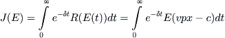 (8.14)
by choosing E properly as some function of time t. The factor e–δt is introduced to indicate that a future gain is worth less than a current profit by an exponential amount. δ is called a discount factor.
The maximum of (8.14) admits an easy solution. Assume, first, that the fishing effort E is constrained to have a maximum value Em, corresponding to a limit on fleet size or total gear that can be deployed per unit time: 0 ≤ E ≤ Em. From (8.12) we see that E = (f(x) – x′)/vx, and so (8.14) can be rewritten as
 (8.15)
Now define Z(x) by the integral
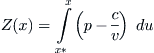
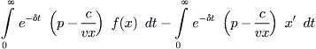
Using an integration by parts, the second integral in (8.15) can be expressed as
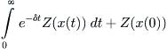
where x(0) is the initial value of x, which we assume to be greater than x∗. As a matter of fact, x(t) will take on values only between K, its maximum population density, and x∗, where the economic incentive to continue fishing is zero. The expression for J(E) is now
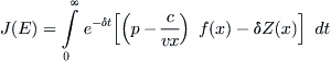 (8.16)
The function F(x) = (p – c/vx)f(x) – δZ(x) that appears in the integrand has a unique positive maximum ![]() somewhere in the interval between x∗ and K. To see this, first note that for any given effort E one has νEx = f (x) at an equilibrium x of (8.12). Therefore, letting q(x) = f(x)(p – c/vx), it follows that q(x) = E(vpx – c), which is the net revenue associated with the equilibrium value of x. As x increases from x∗, the revenue increases to a maximum at some x0 and then decreases. It follows that q′(x) is monotone downward, crossing the x-axis at x0. To find the maximum of F(x), we set F′ to zero to obtain the equation q′(x) = δ(p – c/vx). The curves q′ and δ(p – c/vx) intersect at some
somewhere in the interval between x∗ and K. To see this, first note that for any given effort E one has νEx = f (x) at an equilibrium x of (8.12). Therefore, letting q(x) = f(x)(p – c/vx), it follows that q(x) = E(vpx – c), which is the net revenue associated with the equilibrium value of x. As x increases from x∗, the revenue increases to a maximum at some x0 and then decreases. It follows that q′(x) is monotone downward, crossing the x-axis at x0. To find the maximum of F(x), we set F′ to zero to obtain the equation q′(x) = δ(p – c/vx). The curves q′ and δ(p – c/vx) intersect at some ![]() that lies between x∗ and x0.
that lies between x∗ and x0.
Note that as δ goes to infinity, ![]() tends to x∗. This is what one would expect in view of the fact that δ = ∞ corresponds to completely discounting the future in favor of revenues that are earned immediately. This is the prevalent attitude in a common-access fishery in which, as we have seen, revenue is driven to zero and the biomass level is reduced to x∗.
tends to x∗. This is what one would expect in view of the fact that δ = ∞ corresponds to completely discounting the future in favor of revenues that are earned immediately. This is the prevalent attitude in a common-access fishery in which, as we have seen, revenue is driven to zero and the biomass level is reduced to x∗.
Because J(E) is to be maximized, it is apparent that x(t) should be chosen so that it reaches ![]() from its starting point x(0) as quickly as possible and then remains there for all subsequent time. This is because e–t is a decreasing function of t, and so it is incumbent to reach the maximum value of F(x) as soon as possible. If x is initially greater (lesser) than
from its starting point x(0) as quickly as possible and then remains there for all subsequent time. This is because e–t is a decreasing function of t, and so it is incumbent to reach the maximum value of F(x) as soon as possible. If x is initially greater (lesser) than ![]() , then evidently x′ should be chosen to have the largest possible negative (positive) value. It follows that the optimal harvesting policy for a single owner is
, then evidently x′ should be chosen to have the largest possible negative (positive) value. It follows that the optimal harvesting policy for a single owner is
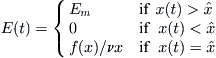 (8.17)
Now suppose that the fishery is limited to a finite number of individuals or firms by the imposition of entry fees or licenses, either of which serves to restrict entry. For simplicity, we consider the case of only two owners who vie with each other to exploit the fishery. Each differs in the values of E, p, c, and v; we indicate this by the subscript i = 1, 2 to distinguish between them. The basic growth Equation (8.11) now becomes
![]() (8.18)
(8.18)
because both owners ply the same waters, and the fish biomass is reduced by their combined efforts. The long-term revenue accrued by each owner is consequently a function of both harvesting rates, and by analogy with (8.14) we write
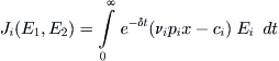 (8.19)
If each owner works separately, without competition from the other, then each would attain an optimal harvesting level ![]() , i = 1, 2, as explained earlier. But in reality they must they seek a competitive equilibrium that compromises the individual goals of maximizing (8.19). A pair of Ei# will be deemed optimal if
, i = 1, 2, as explained earlier. But in reality they must they seek a competitive equilibrium that compromises the individual goals of maximizing (8.19). A pair of Ei# will be deemed optimal if
![]() (8.20)
(8.20)
for all admissible Ei that satisfy 0 ≤ Ei ≤ Ei. This means that if owner 1, for example, unilaterally changes his strategy while owner 2 sticks to his, then J1 either remains the same or, at worst, decreases.
Let xi∗ = ci/vpi. Then owner 1 is more efficient than owner 2 if x1∗ < x2∗. This means that owner 1 operates at lower costs, or fetches higher prices for his catch, or is technologically better equipped. In this case, the competitive equilibrium is given by the rules
 (8.21)
![]() (8.22)
(8.22)
Let us establish the truth of (8.21). The other rule (8.22) is verified in a similar fashion. To begin with, define f1(x) by
![]()
If ![]() is large enough, f1 is negative for
is large enough, f1 is negative for ![]() . Now assume that rule (8.22) holds. Then (8.18) becomes
. Now assume that rule (8.22) holds. Then (8.18) becomes
![]()
By analogy with the way F(x) was defined earlier, let
![]()
in which Z1 is the same integral as Z except that its lower limit is ![]() . It is always true that
. It is always true that ![]() . Moreover, because
. Moreover, because ![]() F1 is maximized by choosing x equal to the smallest of
F1 is maximized by choosing x equal to the smallest of ![]() and
and ![]() because F1(x) is immediately negative as soon as x exceeds
because F1(x) is immediately negative as soon as x exceeds ![]() . The form of F1 in this figure is arrived at from the same considerations that applied to F earlier. We conclude that J1(E1, E2#) must be maximized by rule (8.21), for the reason that J(E) for a single owner was maximized previously using (8.17).
. The form of F1 in this figure is arrived at from the same considerations that applied to F earlier. We conclude that J1(E1, E2#) must be maximized by rule (8.21), for the reason that J(E) for a single owner was maximized previously using (8.17).
The interpretation of this result is that if owner 1 is more efficient, then he drives owner 2 out of business, since x is quickly brought down to a value at which the net revenue to 2 is zero. Since ![]() , the revenue garnered by 1 is positive. When
, the revenue garnered by 1 is positive. When ![]() , owner 1 eliminates his competitor by fishing more intensively than if this inequality is reversed. In effect the first owner must work hard to keep his competitor from returning. Finally, in the case in which x1∗ = x2∗, the revenues of both parties are evidently dissipated to zero, and the situation is no better than in an open-access fishery.
, owner 1 eliminates his competitor by fishing more intensively than if this inequality is reversed. In effect the first owner must work hard to keep his competitor from returning. Finally, in the case in which x1∗ = x2∗, the revenues of both parties are evidently dissipated to zero, and the situation is no better than in an open-access fishery.
In summary, we see that if the goal of limited access is to safeguard against overfishing, it is not a very successful ploy, because the intense competition among participants ensures that the fish stocks will be reduced as far as necessary to achieve the complete elimination of those who are less efficient. This may be recognized as another form of the principle of competitive exclusion that we encountered in Chapter 6. Evidently, some other form of control, such as catch quotas or a tax on the harvest, is required for effective conservation.
8.6 Concluding Thoughts
It is interesting to compare the optimal strategies adopted by the various participants in the previous section. We have no intention of delving into the formalism of game theory, where these matters are discussed in more detail, but only wish to comment, in a slightly more abstract way, on the approaches that were used.
There are two competitors Ci, i = 1, 2, who aim to achieve certain goals but are constrained by the presence of the other. Let G1(u, v) and G2(u, v) represent the loss to each side, where u and v are strategies that are available to C1 and C2, respectively. If C1 is pessimistic, he or she believes that C2 will try to thwart him or her by choosing a strategy v that will maximize the loss G1. Therefore C1 adopts a conservative attitude and picks u to minimize his or her maximum loss. The other competitor, equally suspicious, behaves similarly. Letting u0 and v0 be a pair of optimal strategies for each side, which means that
![]() (8.23)
(8.23)
To see how (8.23) comes about, note that G1(u, v0) = max G1(u, v) ≥ G1(u, v) for all u and v (the maximum is over all v) and, therefore, G1(u0, v0) = minmax G1(u, v) ≥ min G1(u, v) = G1(u0, v), with the minimum taken over all u. A similar set of relations is applicable to G2.
The first inequality in (8.23) expresses the idea that no matter what v is picked by C2, the loss to C1 can never be greater than G1(u0, v0) as long as C1 chooses u0. The second inequality has a similar interpretation. This is known as a minmax strategy. What is being ignored here, of course, is the question as to whether optimal strategies exist to begin with, a mathematical issue that belongs to the domain of game theory.
A different competitive approach is the one adopted by the two owners of a fishery, in which both sides select strategies u0 and v0 so that any unilateral change on the part of C1, say, to some other choice of u can only increase the loss G1, as long as C2 sticks to using v0. Similar considerations apply to C2. This can be expressed as a pair of inequalities:
![]() (8.24)
(8.24)
This is referred to as a Nash competitive strategy.
A comparison of these approaches shows that minmax and competitive strategies need not equal each other, because one is based on pessimism and the other on greed. There is one situation in which the two approaches are equal, however. Suppose that G1(u, v) = –G2(u, v) so that a gain to one side is a loss to the other. Then (8.23) and (8.24) reduce to the same strategy pair. For more details regarding game-theoretic considerations, see the book by Morton [86].
A good source for the exploitation of renewable resources and, in particular, fish harvesting models, is the book by Clark [36]. The model of Section 8.5 is also due to Clark [35].
The notion that a renewable resource such as a fishery, a forest, or grazing lands, which are open to exploitation to all without restriction, will ultimately be devastated in the stampede to exploit it in one’s own interest, without regard to the common good, has been called “the tragedy of the commons” in an elegant article by Garrett Hardin [60].
The fishery problem continues to resurface (for example, see “Northwest fishermen catch everything, and that’s a problem,” New York Times, Nov. 13, 1988), “Commercial Fleets Reduced Big Fish by 90%, Study Says,” New York Times, May 15, 2003, and, most recently, “Odd Alliance Is Forged Over Access to Herring,” New York Times, July 3, 2012, for just a sample of such articles), and so models like the one discussed in Section 8.2 remain appealing even if they are admittedly too simple.