Poisson Events

I want to establish some of the properties of Poisson processes that were employed in Chapters 3 and 6 and were either left unproven there or explained by simple heuristics. Certain standard results, such as the mean and variance of a Poisson distribution, can be found in the books by Ross [99, 100], the ones chosen among the many other possible references in probability that could have been cited.

Note that throughout this appendix I assume a certain familiarity with the notion of conditioning one random variable on another, as explained, for example, in Chapters 6 and 7 of Ross [99] and in Appendix D.

To begin with, let’s return to two results stated but not proved in Section 3.2. First, Let N_i(t) be independent Poisson random variables at rates λ_i, for i = 1, 2, . . . , m. Then the sum N(t) = N₁(t) + N₂(t) + · · · + N_m(t) is also Poisson, at rate λ = λ₁ + λ₂ + · · · + λ_m.

To establish this, begin with the case m = 2. Since the event N(t) = k occurs in k + 1 disjoint ways, namely, N₁(t) = i and N₂(t) = k – i, for i = 0, 1, . . . , k, we can sum over k + 1 events to obtain

Moreover, the separate counting processes are statistically independent, and so the last sum becomes

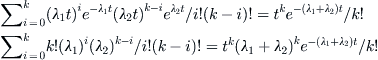
using the binomial theorem. Now proceed by induction. If the sum of the first m – 1 processes is already Poisson, then all we need do is to add the last one to this sum, which is again the case of two Poisson processes considered earlier.

Before I give the next result, recall that a continuous random variable T is said to be exponentially distributed at rate μ if

The expected value of T is readily verified to be 1/μ (Ross [100]), and we show later that the interarrival time between two Poisson arrivals is exponential. I assume that for now, and suppose there are two concurrent and independent Poisson processes at rates μ₁ and μ₂, respectively. A patient observer will see the next arrival from either the first or the second process. The probability that the next occurrence is actually from process i, 1 ≤ i ≤ 2, is μ_i/μ, where μ is the sum μ₁ + μ₂. We prove this in terms of the interarrival times T and T ′ of two simultaneous Poisson processes. Our second result from Section 3.2 is then:

Let T and T′ be independent and exponentially distributed random variables at rates μ₁ and μ₂. These define the interarrival times from two Poisson processes at rates μ₁ and μ₂. The probability that the first arrival occurs from the process having rate i is μ_i/μ, where μ is the sum of μ₁ and μ₂.

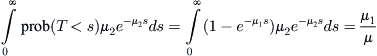
To prove this, let i = 1. A similar argument then applies to i = 2. We need to compute prob(T < T′). The density function of the variable T′ is _, and so, by conditioning on the variable T′, we obtain

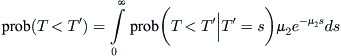
However, since T and T ′ are independent, the last integral becomes

I now want to sketch some details regarding the intimate connection that exists between Poisson processes and the exponential random variables. We need to assume the properties of independence and stationary increments that were detailed in Section 3.2 for a Poisson counting process N(t) having the rate constant λ.

To begin, let P₀(t) denote prob(N(t) = 0). Then P₀(t + h) = prob(N(t) = 0, N(t + h) – N(t) = 0) = P₀(t)P₀(h). But P₀(h) = 1 – prob(N(t) ≥ 1) = 1 – λh + o(h). It follows that [P₀{(t + h) – P₀(t)}]/h = [–P₀(t)λh + o(h)]/h = λP₀(t) + o(h)/h, which tends to –P₀(t)λ as h goes to zero. This gives us the elementary differential equation P₀′(t) = –P₀(t)λ, whose solution is P₀(t) = e^–λt.

Let T₁, T₂, . . . be the interarrival times of the Poisson process in which T₁ is the time of the first arrival, T₂ the time from the first to the second arrival, and so forth. We have just established that T₁ is exponentially distributed since prob(T₁ < t) = 1 – e^–λt. Consider, next, the event T₂ > t. From Appendix D we know, using the expected value, that prob(T₂ > t) = E(prob(T₂ > t|T₁)). But for each sample value s of T₁ we get prob(T₂ > t|T₁ = s) = prob(N(s + t) – N(s) = 0|T₁ = s) = prob(N(t) = 0) = e^–λt. Therefore E(prob(T₂ > t|T₁)) = ∫ e^–λt λe^–λs ds = e^λt. It follows that T₂ is also exponentially distributed and that T₁, T₂ are independent random variables, each having mean 1/λ. By induction this remains true for all interarrival times. Since N(t) is the number of arrivals taking place up to time t, then, as a little thought shows,

if and only if N(t) ≤ n = 1. It follows from this that

which, by differentiation, gives the density function of S_n as

This is known as the gamma density for the random variable S_n, which is the sum of n independent and exponentially distributed variables.

Conversely, suppose that T₁, T₂, . . . are independent and exponentially distributed with a sum S_n that is gamma distributed as previously. Now, prob(N(t) = n) = prob(N(t) ≥ n) – prob(N(t) ≥ n – 1) = prob(S_n ≤ t) – prob(S_n–1 ≤ t) =

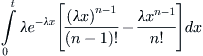
and, consequently, after integrating by parts, we find that prob(N(t) = n) = (λt)ⁿe^–λt/n!, which establishes that N(t) is Poisson-distributed.

The Poisson probability distribution is sometimes considered the most random of random processes. To explain this, suppose that there are exactly N arrivals from a Poisson process on an interval of length T. Then, ignoring their order of appearance, the N arrival times can be obtained by throwing darts at random, that is, as N independent samples from a uniform distribution; the darts are just as likely to penetrate one part of [0, T] as any other. Put another way, the N arrival events are indistinguishable from N points chosen independently in the interval [0, T], with no bias in favor of choosing one part of the interval over another. This means, of course, that the points are unlikely to be evenly distributed; indeed, some parts of the interval will see clumps of points, whereas other segments will be sparsely populated. This is another version of the clustering phenomenon that is so characteristic of randomness.

It is this link between the Poisson and uniform distributions that makes a good fit of empirical data to a Poisson distribution the quintessential tool for inferring the data’s randomness. Because of the significance of this result and because its proof is a bit tricky, I give a detailed argument shortly.

First, however, a random variable X is said to be uniformly distributed on [0, T] if prob(Y ≤ y) = y/T, and its density function f(t) = prob(Y = y) is therefore the constant 1/T. Let Y₁, . . . , Y_n be independent random variables uniformly distributed on [0, T]. Then their joint density function is ∏ f(y_k) = 1/T ⁿ, with k summed from 1 to n.

Define random variables Y_(k) for k = 1, . . . , n, by Y_(k) is the kth-smallest value among the Y_k. That is, if 0 < y₁ < … < y_n < T are values taken on by the Y_k written in increasing order, then Y₍₁₎ = y₁, . . . , Y_(n) = y_n. For example, if n = 3 and Y₁ = 3, Y₂ = 1, Y₃ = 4, then Y₍₁₎ = 1, Y₍₂₎ = 3, Y₍₃₎ = 4.

There are n! distinct ways that the Y_k variables can take on the values y₁ < … < y_n. Suppose that y_j1, . . . , y_jn is one of these permutations. Then

Each of the permutations corresponds to one of n! disjoint events describing how the Y_k variables can take on the values y₁, . . . , y_n. Therefore,

This expression is the density function obtained by ordering in increasing rank the n! distinct possibilities for n independent uniform variables to take on a set of n values. This is known as the ordered statistics of the uniform variables.

Now suppose that there are n arrivals of a Poisson process in [0, T], and let S_k, k = 1, 2, . . . , n + 1 denote the successive gap lengths of these arrivals. That is, if the first and second arrival take place at times s₁ and s₂, then S₁ = s₁ and S₂ = s₂ – s₁, and so forth, with S_n+1 > T – s_n. From Bayes’ rule we find that

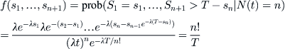
We therefore obtain that the n arrival times of a Poisson process in [0, T], considered as unordered random variables, have the same distribution as the ordered statistics of n independent uniformly distributed random variables. This is the property of randomness that we were seeking, as mentioned earlier.

A similar result holds for spatial Poisson processes. A formal definition of such processes is given in terms of a region R of area A(R) and a function N(R) that counts the number of arrivals in R. Then prob(N(R) = k) = (λA(R))^ke^–λA(R)/k!, where λ is the average number of arrivals per unit area. The probability depends on area but not on the shape of R.

Suppose we know that there is one arrival in R, then the probability that the arrival lies within the subset S is, because of independence, prob(N(S) = 1|N(R) = 1) = prob(N(S) = 1, N(R – A) = 0)/prob(N(R) = 1) = λA(S)e^–λA(S)e^–λ(R-S)/λA(R)e^–λA(R) = A(S)/A(R). That is, the arrival is uniformly distributed within R. The result extends to n arrivals.

In Section 6.6 a statistical technique, the chi-squared test, was introduced to assess whether a set of sample data can be plausibly said to come from a Poisson distribution, namely, if we are willing to reject, with some degree of confidence, the null hypothesis that the data is not Poisson. I want to mention here another simple but rarely quoted test for the uniform distribution of n variables known as Sherman’s statistic, which dates from 1950 (Bartholomew [9]). The setting is familiar. We are given n arrival points x_k in, say, an interval of length T, which results in n + 1 interval gaps between the arrivals, defined by s_k, with s₁ = x₁, s₂ = x₂ – x₁, . . . , s_n+1 = T – x_n. We want to determine if the unordered arrivals are n samples from a uniform distribution on [0, T], and to this end we define a quantity

which measures the deviation between the gap lengths and the average gap T/(n + 1). Note that a large value of w_n is unlikely to arrive by chance, since it would imply that some intervals between events are too large and others too small, which suggests a nonrandom mechanism. On the other hand, a very small value of w_n tells us that the intervals are spaced fairly regularly; again we do not attribute this to happenstance.