
Bioinformatics tool for sequence analysis
In present-day genetics, molecular biology, biomedicine and other areas of the life sciences, computers are used for studying biotic systems and bioprocesses. The discipline involved, bioinformatics, operates through accessing and analysis of information accumulated in formatted databases. For this, MATLAB® offers a specially designed tool – the Bioinformatics toolbox™ containing a set of specialized commands, some of which are discussed in this chapter.
In this context, terms and information relevant to biology, database organization and sequence analysis are given here briefly. For further details, biology and bioinformatics tutorials should be consulted.
6.1 About toolboxes
Although commands and functions such as sin, cos, sqrt, fzero, quard, save, ode45 and pdpde are operative in a wide range of areas from mechanics to medicine, specialized means are needed in each area for its specific problems. Basic and problem-oriented tools are collected in so-called toolboxes intended for particular engineering areas; for example, basic commands are assembled in the MATLAB® toolbox, commands related to signal processing in the Signal Processing toolbox and commands for neural networks in the Neural Network toolbox. To find out which toolboxes are available in your computer, the ver command should be used. Typing this in the Command Window and then entering it, the mathworks product family header information will display together with a list of toolbox names, versions and release. The list can be very long, depending on the MATLAB® configuration on the actual computer:
MATLAB®Version 7.10.0.499 (R2010a)
MATLAB® License Number: 617196
Operating System: Microsoft Windows XP Version 5.1 (Build 2600: Service Pack 3)
Java VM Version: Java 1.6.0_12–b04 with Sun Microsystems Inc. Java HotSpot(TM) Client VM mixed mode
| MATLAB® | Version 7.10 | (R2010a) |
| Simulink | Version 7.5 | (R2010a) |
| AerospaceBlockset | Version 3.5 | (R2010a) |
| Aerospace Toolbox | Version 2.5 | (R2010a) |
| Bioinformatics Toolbox | Version 3.5 | (R2010a) |
The information about toolboxes that is available can also be obtained from the pop-up menu appearing after clicking the Start button in the bottom line of the MATLAB® Desktop – see Figure 2.2.
Initially, bioinformatics was confined to genomics and genetics, in particular DNA sequences. Today, it covers compilation and advancement of databases, algorithms, and computational and statistical techniques.
6.2 The functions of the Bioinformatics toolbox™
The toolbox performs the following functions:
• access to public databases on the Web and other online data sources;
• support formats specific to genomic, proteomic and gene expression data;
• transfer of data, written in different bioinformatics formats, directly to the Workspace for further processing by MATLAB® programs;
• analysis of DNA, RNA and peptide sequences. A sequence represents a frequently very long chain of letters chosen from the four-letter DNA and RNA or 23-letter amino-acid alphabet; for more details see subsection 6.4.1.
• analysis of microarray or phylogenetic data;
• preprocessing of mass spectrometry data;
• reading data generated by gene sequencing instruments, mass spectrometers and microarray scanners;
6.3 Public databases, data formats and commands for their management
Biological information is collected in special formats and can be retrieved from databases that support data exchange and processing. Web-based databases are open to the public and can be copied to and processed on your computer.
6.3.1 Databases to which MATLAB® has access
Currently, the toolbox provides access to the GenBank, GenPept, EMBL, PDB, NCBI GEO and PFAM databases.
GenBank stores an annotated collection of the genetic sequences – it is managed by the National Institute of Health (USA); GenPept contains translated protein-coding sequences – it is managed by the National Center for Biotechnology Information (NCBI), which provides this Entrez system for protein information search; EMBL belongs to the European Molecular Biology Laboratory and stores Europe’s primary nucleotide sequence resources; PDB (Protein Data Bank) stores 3D structural data on large biological molecules, namely proteins and nucleic acids – it is managed by the Worldwide PDB organization; GEO (Gene Expression Omnibus) stores chips, microarrays, gene expression data and hybridization arrays – it is supported by the National Center for Biotechnology Information, NCBI; the GO (Gene Ontology) database stores gene product properties, including the PFAM database that contains information about protein families with their annotations and multiple sequence alignments generated by the hidden Markov model – it is managed by the Wellcome Trust Sanger Institute.
6.3.2 About formats for storage and searching of database information
For each stored substance the data set contains sequences, text, graphs, numbers and other information written in different data formats. For operations with such diverse data MATLAB® uses so-called structures, which are commonly taught in advanced courses; only the minimal information about structures required to use the toolbox commands is provided here.
A structure is constructed from the name of the variable and those of the fields, which are separated from the structure name by a period; for example, s.sequence is the structure named s with the sequence field, and s.molar_weight is the molar_weight field of the same s structure. The fields contain data of different types; for example, in the s structure the sequence field may contain a set of characters of the char type, and the molar_weight may contain a molar-weight value of the double (numerical) type. The number of fields is limited only by the amount of memory. They can contain tables, plots or subfields with data. The structure may be given as a vector, in which case for reading or writing the data, the index of the element should be provided. For example, s(2).sequence means sequence data from the second element of the s structure.
The data are stored in databases in particular form defined by a special file format. Below are some file formats supported by the Bioinformatics toolbox™ for sequence data:
• FASTA is intended for coding nucleotide and peptide sequences represented by single-letter codes;
• PDB is a file format designed for storage of protein information with the 3D structure of protein and nucleic acid molecules;
• SCF (source comparison file) is a format of data transmitted from instruments used for DNA sequencing.
The toolbox also supports additional file formats such as: the Affimetrix DAT, EXP, CEL, CHP, GenePix GRP and GAL for microarray data; Microsoft Excel or CSV for industrial-specific data; and various others for web-based databases. More detailed information is available in the original toolbox documentation.
Working with databases necessitates recourse to specialized algorithms searching for similarity between sequences; the most widespread are FASTA (fast algorithm; the same name as the format described above) and BLAST (Basic Local Alignment Search Tool). FASTA is intended for alignment of DNA and protein sequences, and BLAST for comparing nucleotide or protein sequences with sequence databases and calculating the statistical significance of matches.
6.3.3 Commands for accessing and reading database files
For each format of data stored in a database, MATLAB® offers a set of commands for receiving the data, saving it to a file in the specified format, and reading from the file all previously saved formatted data. For retrieval of information, each biological species has to be assigned an identifier to be obtained from the bank before the request is placed.
For example, nucleotide information may be retrieved from the CenBank© and written into the variable or into the MATLAB® file by following the simplest forms of the getgenbank command:
data = getgenbank(‘accession_number’)
getgenbank(‘accession_number’,’ToFile’, ‘file_name’)
where accession_number is the identifier of a sequence accepted in the bank; ToFile is the property name to be written into the quotes; file_name is a string with file name for saving GenBank data in the current directory, or with the full pass and file name for saving in any other directory; data is a structure that contains information about a sequence received from the bank.
The accession number (called locus number in some databases) is an important attribute that should be defined before transmitting information from a database to the MATLAB® Workspace.
For database exploration and to obtain an accession number, the web command can be used. Its simplest form is
where url (uniform resource locator) is a string defining the Internet address of the searched resource. The web command opens the MATLAB® Web browser with the website indicated by url; for example, if we want to open NCBI databases, we should type and enter in the Command Window:
> > web(‘http://www.ncbi.nlm.nih.gov/’)
The browser window with NCBI home page (Figure 6.1, p. 176) is opened:
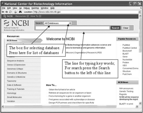
The window provides two Search boxes. For instance, if we need an accession number for stored information about the hexosaminidase A (HEXA) enzyme for the Norway rat, we select ‘Nucleotide’ in the first box pop-up menu (appears after pressing the arrow on the right of the box – see Figure 6.1) and the key words ‘hexosaminidase A Norway rat’ should be typed in the second Search line. The window that is opened is shown in Figure 6.2 (p. 177).
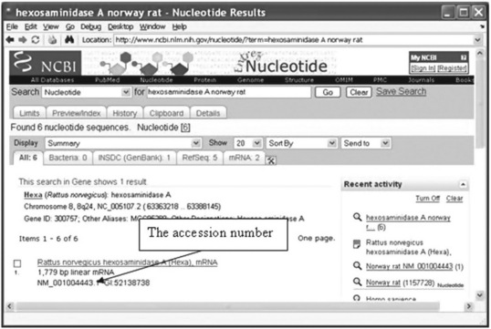
This accession number should be used in the getgenbank command that retrieves sequence information about the Norway rat and transmits it to the S structure:
> > % transmits from database to the S-structure
> > % sequence information about the Norway rat
> > S = getgenbank(‘NM_001004443’)
LocusModificationDate: ‘26-JAN-2010’
Accession: ‘NM_001004443 XM_217144’
Source: ‘Rattus norvegicus (Norwayrat’
To display information contained in one of the fields of the S structure – e.g. in the LocusName and in the SourceOrganism fields – type and enter:
> > display an access number that contains in the LocusName field
> > S. SourceOrganism % display the source organism for this sequence
Eukaryota; Metazoa; Chordata; Craniata; Vertebrata; Euteleostomi; Mammalia; Eutheria; Euarchontoglires; Glires; Rodentia; Sciurognathi; Muroidea; Muridae; Murinae; Rattus.
> > getgenbank(‘NM_001004443’,’ToFile’, ‘Norway_Rat.txt’)
After entering the latter command the same information as in the previous getgenbank example is displayed and saved in the Norway_Rat.txt file generated in the current directory.
The getgenbank command permits retrieval of sequences only from the database:
data = getgenbank(‘Accession_Number’, ‘SequenceOnly’, ‘true’)
For reading files saved as ASCII text files in the GenBank format, the genbankread command is used:
S_data = genbankread(‘file _ name’)
where S_data is a structure with fields corresponding to the GenBank keywords; and file_name is a string with a file name.
An example of this command form usage is:
> > S_data = genbankread (‘Norway_Rat.txt’) % see precede example
> > displays accession number contained in the LocusName field
Some additional commands for database management are shown in Table 6.1.
Table 6.1
Additional commands for database management*
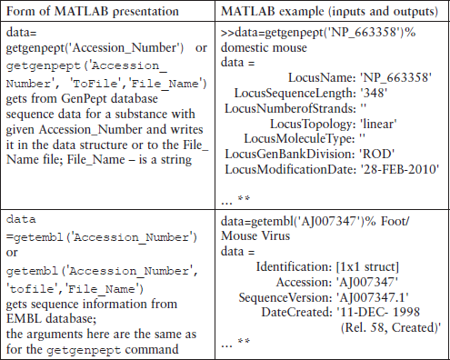
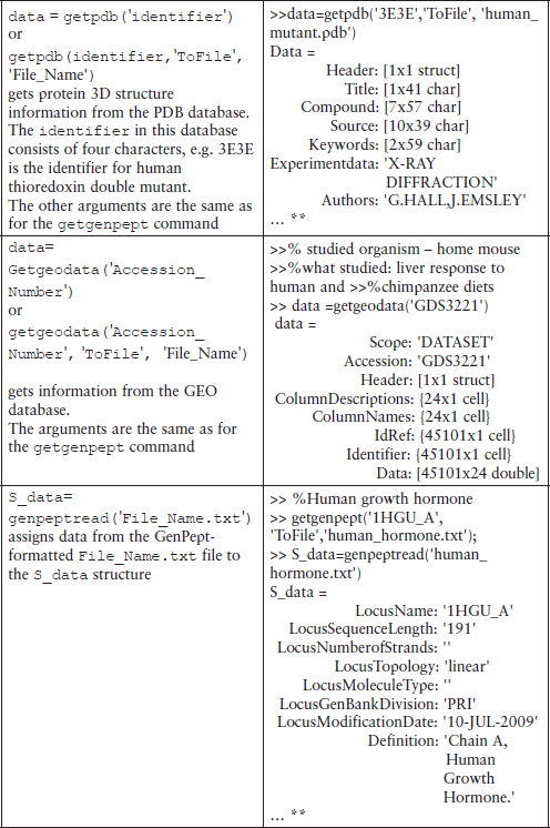
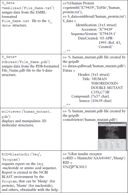
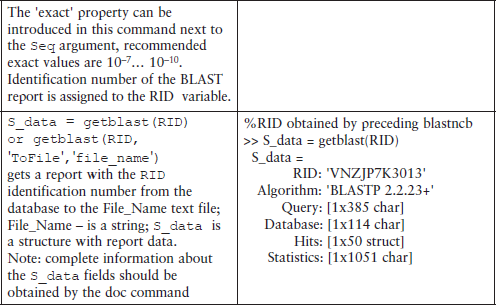
*This table does not contain all possible command forms; for additional information use the help command.
**Shortened.
Each bank access command permits retrieval of a sequence only, which should be done exactly as explained above for the getgenbank command.
6.4 Sequence analysis
Computerized searching and study of nucleotide or amino acid sequence data is termed sequence analysis, which is used for gene identification, detection of inter-gene similarity and gene functions, and search for genecoded proteins. These are realized with commands that fall under three groups - sequence utilities, sequence statistics and sequence alignment.
6.4.1 Sequence utilities and statistics
Utilities
This group of commands serves for manipulation of sequences for more effective use, deeper insight into their characteristics and statistical information.
One command of this group is randseq, frequently used in tests or for explanation of other statistical and analysis commands. It has the form:
Seq_name = randseq(n, ‘alphabet’,’alphabet_name’)
where seq_name is the name of a variable containing the generated string of the letter-code of nucleotides or amino acids; n is a number that specifies the length of the random sequence; ‘alphabet’ is the property specified by the ‘alphabet_name’ value that can be written as ‘dna’, ‘rna’, or ‘amino’ (can also be written as ‘aa’). The ‘dna’ alphabet uses the letters A, C, G and T, the ‘rna’ uses the letters A, C, G and U, the ‘amino’ alphabet uses the letters A, R, N, D, C, Q, E, G, H, I, L, K, M, F, P, S, T, W, Y, V, B, Z and X, and the ‘*’ and ‘-’ symbols.
The ‘dna’ alphabet is a default value; in this case the ‘alphabet’… ‘alphabet_name’ option can be dispensed with.
For example, to generate a protein sequence of 30 letters the following command should be typed and entered in the Command Window:
> > Protein_Seq = randseq(30,’alphabet’,’amino’)
TYNYMRQLVVDVVITNHYSVFATYFSPGFD
Other sequence manipulation commands are those for conversion to sequences using the genetic code. One of these commands is aa2nt, which converts an amino acid sequence to a nucleotide sequence; its simplified form is:
nucleo _seq = aa2nt(amino_seq,’GeneticCode’,code_number,…‘alphabet’, ‘alphabet_name’)
where nucleo_seq is the nucleotide sequence represented by a character string; amino_seq is the string or numeric code specifying the amino acid sequence or the structure with a sequence field containing the amino acid sequence previously retrieved by one of the access or read commands (as described in the preceding subsection); ‘GeneticCode’ is a property specified by the code _number value; and ‘alphabet’ is a property specified by the nucleotide ‘alphabet_name’ string that should be typed as ‘dna’ or ‘rna’. The code_number of the GeneticCode may range from 1 (default value) to 23 and should be chosen from a table obtainable by entering in the Command Window the help aa2nt command. If the ‘dna’ alphabet is used, the ‘alphabet’ option may be dispensed with.
> > nucl_seq1 = aa2nt(‘LifeSciense’,‘alphabet’,‘rna’)
CUCAUUUUUGAGAGUUGCAUUGAGAAUUCUGAA
> > nucl_seq2 = aa2nt(‘LifeSciense’) % default: ‘dna’ alphabet and 1 genetic code
TTAATATTTGAGTCTTGCATTGAGAACAGTGAA
If the converted sequence contains one of ‘*’, ‘-’ or ‘?’, a warning appears:
> > % 2 codes the Vertebrate Mitochondrial
> > nucl_seq = aa2nt(‘BI-SCIENCE’,‘GENETICCODE’,2,‘Alphabet’,’rna’)
Warning: The sequence contains ambiguous characters.
GAUAUU---AGUUGCAUUGAGAACUGUGAA
To perform sequence comparison it is often convenient to transform the nucleotide sequence into a protein sequence, thereby reducing the 64 codons to 20 distinct amino acids. This can be done via the nt2aa command, which has the same form as aa2nt; for example, prot_seq = nt2aa(nucl_seq2) converts the nucl_seq2 nucleotide sequence from one of the preceding examples to the prot_seq protein sequence.
In a gene sequence, non-coding sections may be mixed with exons and determination of a protein-coding sequence can be difficult. To identify the start and stop codons of the protein-coding sequence section (called open reading frame – ORF), you should read the sequence into the workspace with the seqshoworfs command, which defines their positions, assigns the values to a structure with the start and stop fields, and displays the Open Reading Frames window.
Statistical commands
The commands of this group are intended for statistical problems: nucleotide, codon, dimer and amino-acid counts in sequences, molar weight determination, calculation and plotting of nucleotide density changes along the sequence, graphical representation, etc.
As an example, we consider the aacount command that counts, displays and plots the amount of each amino acid in the sequence. Its simplified form is:
amino_s = aacount(amino_seq,‘chart’,chart_value)
where the amino_seq is a letter string or a row vector of integer numbers representing an amino acid sequence, or a structure with a sequence field that contains such a sequence previously constructed by the appropriate command described in Subsection 6.3.3; the ‘chart’ property is specified by the chart_value, and can be ‘pie’ or ‘bar’ depending on the desired graphical representation; the ‘chart’-chart_value option can be dispensed with – in this case the graph is not generated; the amino_s is a structure containing 20 fields for each of the standard amino acids.
Below are versions of the aacount command:
> > % generation of the 25 letter sequence
> > seq = randseq(25,‘alphabet’,’amino’)
> > returns amount of Tryptophan (W) in the seq sequence
> > assigns results to amino-acid and plots
The first command of the example generates a random sequence of the amino acid letter codes and assigns the result to the seq variable. The second aacount command counts the amount of each amino acid in the sequence, assigns it to the appropriate fields of the amino_acid structure and generates the plot shown in Figure 6.3.
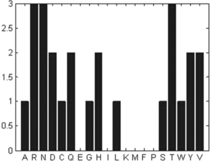
Figure 6.3 Bar chart of amino acid amounts produced by the aacount command for a randomly generated 25-letter sequence.
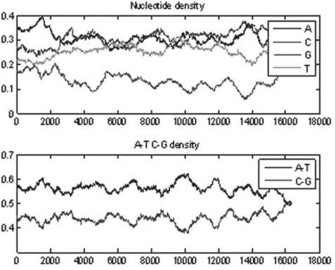
Another command of the statistical group is the ntdensity, which counts and plots the density of the A, C, G and T nucleotides. Its simplest form is:
nucl_dens = ntdensity(nucleotide_seq)
where nucl_dens is a structure with the fields A, C, G and T containing their densities; the nucleotide_seq is a letter string or a row vector of integer numbers representing a nucleotide sequence, or a structure with a sequence field that contains nucleotide sequence previously constructed by an appropriate command described in Subsection 6.3.3.
> > % get data for rhesus macaque
> > macaque = getgenbank(‘NM_001168654’,’sequenceonly’,‘true’);
> > nucl_dens = ntdensity(macaque)
The getgenbank command in this example retrieves the sequence for rhesus macaque semenogelin from the GenBank database and assigns the results to the macaque variable; the ntdensity command counts the A, C, G and T nucleotide density changes along the sequence, assigns them to the appropriate fields of the nucl_dens structure and generates the plots in Figure 6.4.
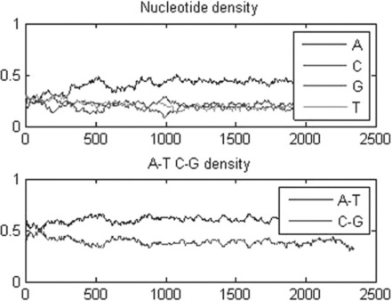
Figure 6.4 A, C, G, T and A, T, C, G nucleotide density plots generated by the ntdensity command for the rhesus macaque semen sequence.
Some additional utility and statistical commands are presented in Table 6.2.
6.4.2 Sequence alignment
The sequence alignment technique is used to search for functional, structural or evolutional similarity between sequences. As sequences are represented by a letter-coded row, the alignment consists of letter-by-letter comparison of two or more sequences.
The Bioinformatics toolbox provides a number of possibilities for alignment of paired and multiple sequences.
Pairwise alignment
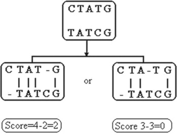
In the process of alignment, gaps can be inserted into the sequences and characters can be inserted and/or deleted. The degree of identity of the sequences is measured by an alignment score criterion. A DNA example is shown in Figure 6.5, with matched characters (vertical bars) graded 1, mismatched characters and inserted gaps by − 1.1 The maximal score means the best alignment.
When two sequences are compared, a matrix is formed in which each row represents a character from one sequence and each column a character from the other; the numbers at a row-column intersection are the similarity score of the row and column character related to this intersection. The path through the maximal score values is the winning path, representing the best alignment. There are PAM, BLOSUM and other widely used scoring matrices for sequence alignment. In multiple alignments distance scores are used; in this case each pairwise score represents the grade of non-identical characters in the compared sequences.
Comparison of sequence alignments achieved via the various scoring systems can be improved by normalizing the scored values and the statistical properties of the system, which makes for non-integer score values. For evaluation of score reliability two statistical indices are often used – probability P and expected value E. A high level of sequence similarity is associated with a high P value (e.g. 90%) and a low E value (e.g. 10- 7), indicating that it is unlikely for the alignment to be randomly successful. The example in Figure 6.5 involves very short sequences, which can be processed manually; real-life biological sequences are significantly longer and require specialized algorithms, classified as global and local. In the first case the goal is total sequence similarity and in the second the goal is to identify regions of similarity within the sequences.
For global alignment the Needleman–Wunsch algorithm is used; this performs by the nwalign command, whose simplest form is
[score,alignment] = nwalign(seq _1,seq _2,’showscore’,true)
where seq_1 and seq_2 are the names of variables containing two amino acids or nucleotide sequences; the ‘showscore’ property with argument true (written without quotes) opens the Figure window displaying the scoring space and the winning path of the alignment. The color of each cell in the scoring space map represents the best score determined over all possible alignments. The winning path is represented by black dots and is shown as the best position of the letter pairs; the color of the lower right cell of the winning path represents the optimal global alignment score, whose numerical value is transmitted to the score variable; score is optimal global score in bits; the alignment is a three-row array which displays in the first and third rows the seq_1 and seq_2 sequences, respectively, and in the second row the ‘I’, ‘:’ or space symbols signing exactly matched (appear in red), mismatched (accepted as related by the scoring matrix, appear in magenta) and non-matched (zero or positive score, appear in black) letters.
In the presented form of nwalign, the BLOSSOM50 (default) scoring matrix is used for amino acids. Its expanded form can use other scoring matrices and some additional scoring and sequence characteristics; for detailed information, type the help nwalign command in the Command Window.
The command can be used without the ‘showscore’ property, in which case only the score value and three rows of the alignment matrix are displayed in the Command Window.
An example for this command is:
> > sequence should contain the letters of the ‘amino’ alphabet
> > s_2 = ‘sefesici’; % the same requirement as for the s_1 >>
[score, alignment] = nwalign(s_1, s_2, ‘showscore’,true)
After entering the latter command the Figure window appears (Figure 6.6) with the scoring space and winning path:
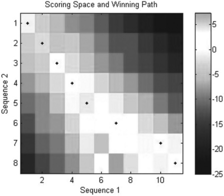
Figure 6.6 Scoring space heat map (colored cells and bar, to the right) and winning path (closed circles) generated with the nwalign command.
To align nucleotide sequences with this command the ‘alphabet’ property with the ‘nt’ argument should be added; for example, the last command in the preceding example can be rewritten as
[score, alignment] = nwalign(s _1, s_ 2, ‘showscore’,true, ‘alphabet’, ‘nt’)
where s_1 and s_2 are assumed here to be nucleotide sequences.
For local alignment the Smith–Waterman algorithm is used. This is realized in the swalign command
and is similar to the previous command:
[score,alignment] = swalign(seq _1,seq _2,’showscore’,true)
All input and output parameters here are the same as for the nwalign command with the only difference that the output values are the results of the local not the global alignment.
An example of this command application is:
> > % s1,s2 are the same as in the nwalign
> > [score, alignment] = swalign(s_1,s_2,’showscore’,true)
The resultant map (Figure 6.7) is:

Figure 6.7 Scoring space heat map (colored cells and bar, to the right) and winning path (closed circles) generated with the swalign command.
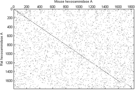
Another graphical representation, often used for comparison of protein sequences, is the dot plot, sometimes called the residue contact map. The compared protein sequences are located along the vertical and horizontal axes, and identical proteins are shaded in black. If the plot clearly shows a diagonal line, the alignment is good. For generation of a dot plot the seqdotplot command is used:
seqdotplot(seq_1,seq_2,window,number)
where seq_1 and seq_2 are nucleotide or amino acid strings or structures with the sequence field obtained from a sequence database; window and number are integer numbers that define the size of a window and the number of characters that should be matched within it. For nucleotide sequences window is often taken as 11 and number as 7.
> > mouseHEXA = getgenbank(‘AK080777’,’sequenceonly’,true);
> > ratHEXA = getgenbank(‘NM_001004443’,’sequenceonly’,true);
> > seqdotplot(mouseHEXA,rathexa,11,7)
Warning: Match matrix has more points than available screen pixels.
Scaling image by factors of 2 in X and 2 in Y
> > xlabel(‘Mouse hexosaminidase A’);
> > ylabel(‘Rat hexosaminidase A’);
In this example the nucleotide sequences for domestic mouse and Norway rat hexosaminidase A are obtained by the getgenbank command. The warning gives here information about the factors used for scaling of the axis. The plot generated by the seqdotplot command is shown in Figure 6.8 (p. 195).
Multiple alignment
Alignment of three or more biological sequences can be done via multiple alignment, which is used for analyses of evolutionary relationships. One of the commands used for this is multialign, which uses the progressive method (the hierarchical or tree method) and has the following simplest form:
aligned_seqs = multialign(sequence_set)
where aligned_seqs is a structure or character array output with the aligned sequences; sequence_set can be a structure or a character array.
Its expanded form may contain the relationships among sequences; by default the command defines distance scores and forms relationships between sequences called the phylogenetic or guide tree.
> > seqs = strvcat(‘CGTTAT’,’TCGTTAC’,’TAGTTGTGC’,’GAGTTAATG’);
The first command of this example assigns to the seqs an array with four sequences containing DNA letters, and the second shows the results of the multiple alignment.
More complicated command forms for scoring matrices, user-given trees, gap-score values and others can be obtained by typing and entering the help multialign command.
For better graphical representation of aligned sequences the showalignment(aligned_seq) command is used. For example, an alignment executed by the > > [Score, Alignment] = nwalign(‘LIFESCIENCE’, ‘SERIES’); can be represented by typing and entering in the Command Window
The Aligned Sequences window appears (Figure 6.9):
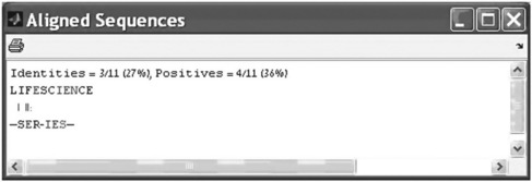
For pairwise alignment the matched and unmatched characters appear respectively in red and magenta.
The graphical representation of multiple alignment (Figure 6.10 shows alignment of four sequences) given in the previous multialign example can be obtained by typing and entering
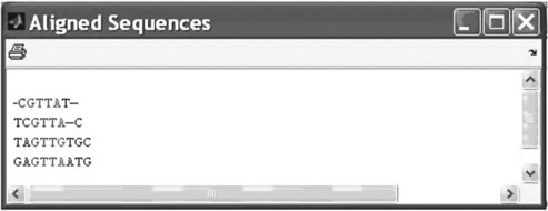
The columns with highly conserved characters are highlighted and appear in red and conserved characters in magenta.
For long sequences (longer than 64 characters) another form of the showalignment command should be used:
showalignment(Alignment, ‘Columns’, Columns_Value)
where Columns_Value of the ‘Columns’ property is the maximal integer number of characters showing in one line; for example, showalignment(Alignment, ‘Columns’, 64) displays up to 64 letters on one line.
Another command that may be used to display multiple alignments is:
where alignment is a structure with the following fields: Sequence, which is obligatory, and Header, which is optional and is used to display the names of species.
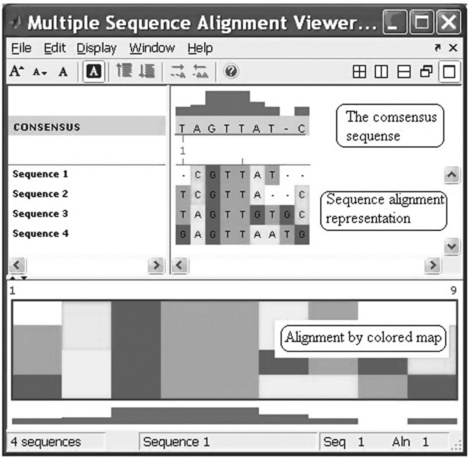
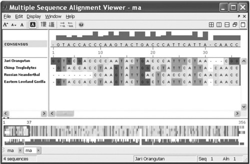
the command opens a viewer that shows the multiple sequence alignment. For example, typing and entering in the Command Window
the Multiple Sequence Alignment Viewer appears with four aligned sequences (Figure 6.11, p. 197).
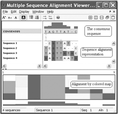
Figure 6.11 Multiple Sequence Alignment Viewer with four aligned sequences generated with the multialignviewer command.
The multialignviewer command was used in this example with the ma variable, which contains the results of the preceding multiple alignment of four short sequences.
With the Multiple Sequence Alignment Viewer you can also interactively adjust a sequence alignment.
Note: Multiple alignment algorithms do not always lead to optimal results and often need some adjustment. More detailed information on this and other subjects of multiple alignments can be obtained in the appropriate sections of the Bioinformatics toolbox user guide.
6.5 Sequence analysis examples
The examples below show how to apply the commands presented above to some problems in sequence statistics and alignment of paired and multiple sequences.
6.5.1 Example of sequence statistics
Problem: Retrieve the sequence information for the western gorilla (Gorilla gorilla) mitochondrion genome from an online database and determine the mono–, di- and trinucleotide contents with sequence statistics commands.
The first step is to determine the access number for this genome. For this we use the web command and explore the NCBI databases. In the Command Window type and enter:
> > web(‘http://www.ncbi.nlm.nih.gov/’)
The NCBI website home page appears in the Web Browser window (Figure 6.1). Then select the ‘Genome’ option in the first ‘Search’ line, type gorilla mitochondrion into the second Search line and press the ‘Search’ button. The following window appears.
The required accession number is NC_001645, which on clicking provides the information shown at the top of p. 200.
The second step consists of retrieving sequence information from the database to the MATLAB® workspace. For this, type in the Command Window:
> > gorilla_mito = getgenbank(‘NC_001645’,’sequenceonly’,true)
GTTTATGTAGCTTACCTCCCCAAAGCAATACACTGAAAATGTTTCGACGGGCTCACATCACCC…
The nucleotide sequence from the GenBank database is assigned to the gorilla_mito variable. Information about its size can be obtained by the whos command (see p. 218):
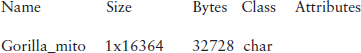

Thus the sequence size is 16,364 characters, equivalent to 32,728 bytes.
With the sequence written in the MATLAB® workspace, we can use the following sequence statistics command:
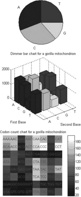
> > figure, basecount(gorilla_mito,’chart’,’pie’)
> > title(‘Nucleotide pie chart for a gorilla mitochondrion’)
> > figure, dimercount(gorilla_mito,’chart’,’bar’)
> > title(‘Dimer bar chart for a gorilla mitochondrion’)
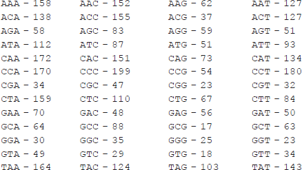
> > codoncount(gorilla_mito,’figure’,true)
![]()
> > title(‘Codon count chart for a gorilla mitochondrion’)
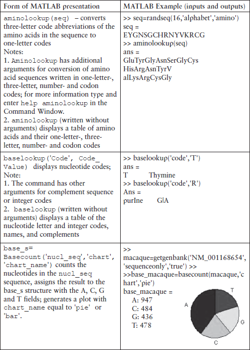
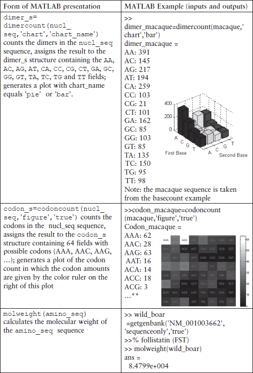
The first command plots the densities of monomers and combined monomers in the Figure window; two commands of the second command line count the nucleotides, display the values counted and show their distribution on the pie plot in the separate Figure window. The title is generated with the third command line; two commands from the fourth command line count the dimers, display the resulting values and generate the bar chart in the separate Figure window. The title is created here with the fifth command line. The final commands count the codons in the first reading frame, display the resulting values and generate the titled graphical table (heat map). The graphs generated are presented below:
6.5.2 Pairwise alignment example
Problem: Use of primates (chimpanzee, gorilla, etc.) as model organisms for studying human diseases is quite expensive because of the various difficulties involved in acquiring specimens. Hence the need for more accessible alternatives. An example is the search for an organism possessing the enzyme hexosaminidase A (HEXA). The procedure described below assumed that:
• the rat genome is a likely candidate,
• the portions of sequences that should be aligned are the third ORF of the human sequence and the first ORF of the rat sequence.
The problem can be solved via an alignment algorithm in the following steps:
• obtain the accession number for the human gene HEXA;
• obtain the accession number for the rat gene HEXA;
• retrieve the human protein coding sequence from a database and save in the MATLAB® workspace;
• retrieve the rat protein coding sequence from a database and save in the MATLAB® workspace;
web(‘http://www.ncbi.nlm.nih.gov/’)
As the first step open the NCBI website by typing and entering in the Command Window:
The NCBI home page appears in the Web Browser window. Now, for example, the Gene option should be selected for the first ‘Search’ box and the Human hexosaminidase A should be typed into the second box.
Press the ‘Search’ button, after which the following window appears (p. 205, top):
As can be seen, the accession number for human (Homo sapiens) HEXA is NM_000520.
Analogously, to obtain the accession number for the Norway rat, select the Nucleotide option in the first box of the Search engine on the NCBI home page and type Norway rat hexosaminidase A in the second box. After pressing the ‘Search’ button we have the following window (p. 205, bottom):
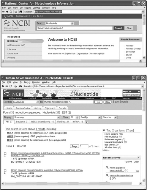
The accession number for brown rat (Rattus norvegicus) HEXA is NC_005107.
The next stage is transferring the nucleotide sequences from the GenBank database to the MATLAB® workspace:
> > hum_hexa = getgenbank(‘NC_006482’,’sequenceonly’,true);
> > rat_hexa = getgenbank(‘NM_001004443’,’sequenceonly’,true);

It is now possible to convert the nucleotide sequences into their amino acid counterparts. In accordance with the problem conditions, the third ORF for the human and the first ORF for the rat should be used. The appropriate commands are
> > hum_protein = nt2aa(hum_ORF,’frame’,3);
> > rat_protein = nt2aa(rat_ORF);
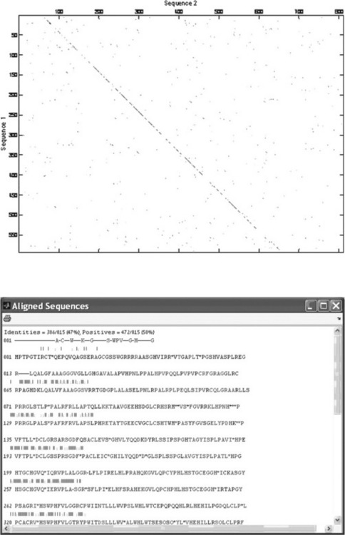
For a visual check of similarity, the dot plot can be used (p. 207, top): > > seqdotplot(rat_protein,hum_protein,4,3)
The diagonal line on the generated plot shows apparently good alignment of the two sequences.
We can now use the Needleman–Wunsch algorithm for global alignment of the two amino acid sequences:
> > [rat_hum_Score, rat_hum_align] = nwalign(rat_protein,hum_protein);
> > for generation of the graphical output
> > showalignment(rat_hum_align)
The resultant Aligning Sequence window (p. 207, bottom) shows that the calculated identity of the studied sequences is 47%.
6.5.3 Multiple alignment example
Problem: To compare the genetic variability, evolution and other relationships among Hominidae, multiple sequence alignment can be used. The task here is to write and save the script file with the name HuminidaeEx.m that is intended to retrieve, align and show results for four Hominidae mitochondrial DNA (D-loop) sequences – orangutan, chimpanzee, Neanderthal and gorilla. The necessary accession numbers are:
Russian Neanderthal – AF254446,
Eastern Lowland Gorilla – AF050738.
The problem will be solved in the following steps:
• Retrieve the sequences from the NCBI database to the Workspace for the mitochondrial DNA (D-loop) of each of the four Hominidae; this can be done with a loop, at each pass of which the accession number in the getgenbank command is changed.
• Align the sequences with the multialign command.
• Show the results in the Multiple Sequence Alignment Viewer by the multialignviewer command.
The script file with the solution of this problem is:
accession_number = [‘AF451964’;’AF176766’;’AF254446’;’AF176731’];
name = strvcat(‘Jari Orangutan’,’Chimp Troglodytes’,…
‘Russian Neanderthal’,’Eastern Lowland Gorilla’);
primate(i).Sequence = getgenbank(accession_number(i,:),’sequenceonly ‘, ‘true’);
primate(i).Header = name(i,:);
The sequences and primate names are contained in the primate structure in the fields named Sequence and Header; these names are required by the multialignviewer command to display the sequences and their
names in the Multiple Sequence Alignment Viewer. After running this file, the window with the four aligned sequences appears:
Retrieval of numerous sequences by the getgenbank command may be time-consuming and without guaranteed success. It is therefore preferable to save previously retrieved information in a file, and retrieve the sequence data from it for subsequent multiple alignments.
6.6 Questions for self-checking and exercises
1. Which of the given commands may be used for global alignment of two sequences: (a) swalign; (b) nwalign; (c) showalignment; (d) aa2nt?
2. The randseq(20) command generates: (a) a random sequence containing 20 letters of the amino acid alphabet; (b) a 20-letter RNA random sequence; (c) a 20-letter DNA random sequence?
3. The dens = ntdensity(seq) command is intended for: (a) counting amino acid densities in the seq sequences and assigning the results to the dens structure; (b) counting the density of the A, C, G and T nucleotides in the seq and assigning the results to the A, C, G, T fields of the dens structure?
4. For conversion of an amino acid sequence into a nucleotide sequence the following command is used: (a) nt2aa; (b) aa2nt; (c) inv; (d) multialign?
5. For counting codons in a nucleotide sequence the following command should be used: (a) basecount; (b) codonbias; (c) dimercount; (d) codoncount?
6. With the MATLAB® Web Browser find in the NCBI GenBank the accession number of the ring-tailed lemur (Lemur catta) clone LB2- 212 N12, retrieve the stored data, save it in the file Lemur.txt, and read the sequence from the appropriate field of the structure stored in this file.
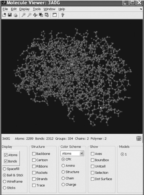
7. Retrieve from the PDB database the stored information about the guinea-pig’s oxyhemoglobin – accession number 3AOG; save the data in a file and display the 3D molecular structure. Write all commands in a script file.
8. Get the nucleotide sequence total data set for the olive baboon (Papio anubis) clone RP41-187H19 stored in EMBL – accession number AC091381; save it in a file, count the nucleotide densities and bases in the sequence, and display the bases in a pie chart. Add the titles ‘Olive baboon clone nucleotide density’ and ‘Olive baboon clone A-T C-G density’ to the appropriate density subplots and the title ‘Nucleotide amounts in the Olive baboon clone’ to the pie chart. Write all commands in a script file.
9. Write a script file that gets the sequence for mouse insulin receptor (accession number NP_034698 in the GenPept database) and use it as a query sequence in the NCBI BLAST search for alignment of this sequence with those of other species (subject sequences) determined by the BLAST search initiated by a MATLAB® command with 1e-7 E value of the ‘expect’ property; place the BLAST report into the Workspace and display in the Command Window the names of the species that were compared with the query sequence; these names are stored in the Hits.Name field.
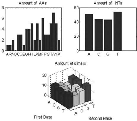
10. Write a script file containing the commands that: (a) generate a random 64-letter amino acid sequence, count the amino acids in it, display the results and generate the bar chart; (b) convert the amino acid sequence into nucleotides, count the nucleotides and dimers in the sequence, and generate the bar charts for nucleotides and dimers. Present all three charts in the same plot; add titles for each chart.
11. From the GenPept database get two protein sequences – for yeast and Escherichia coli, whose accession numbers are 1S1I_C and 1GLA_G, respectively. Write a script file for global pairwise alignment of these sequences, display the score and the aligned sequences in the Command Window, and generate a graph with scoring space and winning path.
12. Write a function file for global pairwise alignment of two protein sequences retrieved from GenBank – score and scoring matrix should be displayed; take as input arguments two strings with accession numbers; calculate and display the scoring space and winning path (in a separate window) and score value (in the Command Window) for two residues: Rhesus macaque (Macaca mulatta) and human cystic fibrosis transmembrane conductance regulator gene, exon 13; the accession numbers for their nucleotide sequences are AF016937 and M55118, respectively.
13. Solve the preceding problem realizing both global and local pairwise sequence alignment in a single function file; introduce the input argument N that allows you to select the desired alignment type: global for N = 1 and local for N ≠ 1.
14. Write a script file with commands that retrieve (from the GenBank database) nucleotide sequences for the mouse (Mus musculus) and human (Homo sapiens) hexosaminidase A genes – accession numbers AK080777 and NM_000520, respectively - convert these sequences into the corresponding amino acid sequences, execute global pairwise alignment, display the scoring space and winning path in a separate window, and display the score value in the Command Window.
15. Get nucleotide sequences from the GenBank database for the cystic fibrosis transmembrane conductance regulator (CFTR) of:
bull (Bos taurus) - accession number NM_174018,
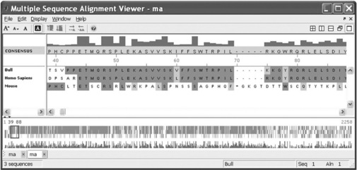
Convert nucleotide into protein sequences; execute multiple alignment and present the results in the Alignment Sequences window. Write all commands in a script file.
6.7 Answers to selected exercises
2.(c) a 20-letter DNA random sequence.
ExperimentData: ‘X–RAY DIFFRACTION’ Authors:
‘ S.ETTI,G.SHANMUGAM,P.KARTHE,K.GUNASEKARAN’
| RevisionDate: | [1x1 struct] |
| Journal: | [1x1 struct] |
| Remark2: | [1x1 struct] |
| Remark3: | [1x1 struct] |
| Remark4: | [2x59 char] |
| Remark100: | [3x59 char] |
| Remark2 0 0: | [49x59 char] |
| Remark2 8 0: | [7x59 char] |
| Remark2 9 0: | [48x59 char] |
| Remark300: | [6x59 char] |
| Remark350: | [27x59 char] |
| Remark4 65: | [11x59 char] |
| Remark4 7 0: | [7x59 char] |
| Remark5 0 0: | [100x59 char] |
| Remark62 0: | [28x59 char] |
| Remark800: | [17x59 char] |
| Remark900: | [7x59 char] |
| dBReferences: | [1x2 struct] |
| SequenceConflicts: | [1x3 struct] |
| Sequence: | [1x2 struct] |
| Heterogen: | [1x4 struct] |
| HeterogenName: | [1x2 struct] |
| HeterogenSynonym: | [1x1 struct] |
| Formula: | [1x3 struct] |
| Helix: | [1x18 struct] |
| Link: | [1x6 struct] |
| Site: | [1x1 struct] |
| Cryst1: | [1x1 struct] |
| OriginX: | [1x3 struct] |
| Scale: | [1x3 struct] |
| Model: | [1x1 struct] |
| Connectivity: | [1x94 struct] |
| Master: | [1x1 struct] |
| SearchuRL: | 3A0G |
12.
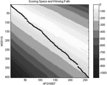
> > score = Ch5_12(‘AF016937’,’M55118’,2)
1Other grading modes are possible, for example 2 for matches and − 1 for mismatches/inserts.