
Continuing our discussion of software reliability models, in this chapter we cover the class of models called the reliability growth models. We first discuss the exponential model; then we concisely describe several notable reliability growth models in the literature; and in later sections we discuss several issues such as model assumptions, criteria for model evaluation, the modeling process, the test compression factor, and estimating the distribution of estimated field defects over time.
In contrast to Rayleigh, which models the defect pattern of the entire development process, reliability growth models are usually based on data from the formal testing phases. Indeed it makes more sense to apply these models during the final testing phase when development is virtually complete, especially when the testing is customer oriented. The rationale is that defect arrival or failure patterns during such testing are good indicators of the product’s reliability when it is used by customers. During such postdevelopment testing, when failures occur and defects are identified and fixed, the software becomes more stable, and reliability grows over time. Therefore models that address such a process are called reliability growth models.
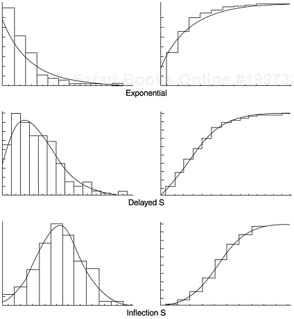
The exponential model is another special case of the Weibull family, with the shape parameter m equal to 1. It is best used for statistical processes that decline monotonically to an asymptote. Its cumulative distribution function (CDF) and probability density function (PDF) are
where c is the scale parameter, t is time, and λ=1/c. Applied to software reliability, λ is referred to as the error detection rate or instantaneous failure rate. In statistical terms it is also called the hazard rate.
Again the preceding formulas represent a standard distribution—the total area under the PDF curve is 1. In actual application, the total number of defects or the total cumulative defect rate K needs to be multiplied to the formulas. K and lambda (λ) are the two parameters for estimation when deriving a specific model from a data set.
The exponential distribution is the simplest and most important distribution in reliability and survival studies. The failure data of much equipment and many processes are well described by the exponential distribution: bank statement and ledger errors, payroll check errors, light bulb failure, automatic calculating machine failure, radar set component failure, and so forth. The exponential distribution plays a role in reliability studies analogous to that of normal distribution in other areas of statistics.
In software reliability the exponential distribution is one of the better known models and is often the basis of many other software reliability growth models. For instance, Misra (1983) used the exponential model to estimate the defect-arrival rates for the shuttle’s ground system software of the National Aeronautics and Space Administration (NASA). The software provided the flight controllers at the Johnson Space Center with processing support to exercise command and control over flight operations. Data from an actual 200-hour flight mission indicate that the model worked very well. Furthermore, the mean value function (CDF) of the Goel-Okumoto (1979) nonhomogeneous Poisson process model (NPPM) is in fact the exponential model.
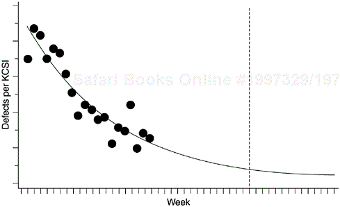
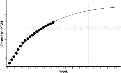
Figures 8.1 and 8.2 show the exponential model applied to the data of one of the AS/400 software products. We have modeled the weekly defect arrival data since the start of system test, when the development work was virtually complete. The system-testing stage uses customer interfaces, tests external requirements, and simulates end-user application environments. The pattern of defect arrivals during this stage, therefore, should be indicative of the latent defect rate when the system is shipped.
Like the Rayleigh model, the exponential model is simple and quick to implement when powerful statistical software is available. For example, it can be implemented via SAS programs similar to the one shown in Figure 7.5 of the previous chapter. Of course, if a high degree of usability and various scenarios are desired, more elaborate software is needed.
Besides programming, the following should be taken into consideration when applying the exponential distribution for reliability projection or estimating the number of software defects. First, as with all types of modeling and estimation, the more accurate and precise the input data, the better the outcome. Data tracking for software reliability estimation is done either in terms of precise CPU execution time or on a calendar-time basis. Normally execution-time tracking is for small projects or special reliability studies; calendar-time tracking is common for commercial development. When calendar-time data are used, a basic assumption for the exponential model is that the testing effort is homogeneous throughout the testing phase. Ohba (1984) notes that the model does not work well for calendar-time data with a nonhomogeneous time distribution of testing effort. Therefore, this assumption must be examined when using the model. For instance, in the example shown in Figures 8.1 and 8.2 the testing effort remained consistently high and homogeneous throughout the system test phase; a separate team of testers worked intensively based on a predetermined test plan. The product was also large (>100 KLOC) and therefore the trend of the defect arrival rates tended to be stable even though no execution-time data were available.
To verify the assumption, indicators of the testing effort, such as the person-hours in testing for each time unit (e.g., day or week), test cases run, or the number of variations executed, are needed. If the testing effort is clearly not homogeneous, some sort of normalization has to be made. Otherwise, models other than the exponential distribution should be considered.
As an example of normalization, let us assume the unit of calendar time is a week and it is clear that the weekly testing effort is not homogeneous. Further assume that weekly data on the number of person-hours in testing are known. Simple adjustments such as the following can reduce artificial fluctuations in the data and can make the model work better:
Accumulate the total person-hours in testing for the entire testing phase and calculate the average number of person-hours in testing per week, n.
Starting from the beginning of testing, calculate the defect rates (or defect count) for each n person-hour units. Allocate the defect rates to the calendar week in sequence. Specifically, allocate the defect rate observed for the first n person-hours of testing to the first week; allocate the defect rate observed for the second n person-hours of testing to the second week, and so forth.
Use the allocated data as weekly input data for the model.
Second, the more data points available, the better the model will perform— assuming there is an adequate fit between the model and the data. The question is: When the test is in progress, how much data is needed for the model to yield reasonably adequate output? Ehrlich and associates (1990) investigated this question using data from AT&T software that was a transmission measurement system for remote testing of special service circuits. They assessed the predictive validity of the exponential model with data at 25%, 50%, 60%, 70%, and 80% into test, and at test completion. They found that at 25% into test the model results were way off. At 50% the results improved considerably but were still not satisfactory. At 60% into test, the exponential model had satisfactory predictive validity. Although it is not clear whether these findings can be generalized, they provide a good reference point for real-time modeling.
The exponential model can be regarded as the basic form of the software reliability growth models. For the past two decades, software reliability modeling has been one of the most active areas in software engineering. More than a hundred models have been proposed in professional journals and at software conferences, each with its own assumptions, applicability, and limitations. Unfortunately, not many models have been tested in practical environments with real data, and even fewer models are in use. From the practical software development point of view, for some models the cost of gathering data is too expensive; some models are not understandable; and some simply do not work when examined. For instance, Elbert and associates (1992) examined seven reliability models with data from a large and complex software system that contained millions of lines of source code. They found that some models gave reasonable results, and others provided unrealistic estimates. Despite a good fit between the model and the data, some models predicted the prob-ability of error detection as a negative value. The range of the estimates of the defects of the system from these models is incredibly wide—from 5 to 6 defects up to 50,000.
Software reliability growth models can be classified into two major classes, depending on the dependent variable of the model. For the time between failures models, the variable under study is the time between failures. This is the earliest class of models proposed for software reliability assessment. It is expected that the failure times will get longer as defects are removed from the software product. A common approach of this class of model is to assume that the time between, say, the (i − 1)st and the ith failures follows a distribution whose parameters are related to the number of latent defects remaining in the product after the (i − 1)st failure. The distribution used is supposed to reflect the improvement in reliability as defects are detected and removed from the product. The parameters of the distribution are to be estimated from the observed values of times between failures. Mean time to next failure is usually the parameter to be estimated for the model.
For the fault count models the variable criterion is the number of faults or failures (or normalized rate) in a specified time interval. The time can be CPU execution time or calendar time such as hour, week, or month. The time interval is fixed a priori and the number of defects or failures observed during the interval is treated as a random variable. As defects are detected and removed from the software, it is expected that the observed number of failures per unit time will decrease. The number of remaining defects or failures is the key parameter to be estimated from this class of models.
The following sections concisely describe several models in each of the two classes. The models were selected based on experience and may or may not be a good representation of the many models available in the literature. We first summarize three time between failures models, followed by three fault count models.
The Jelinski-Moranda (J-M) model is one of the earliest models in software reliability research (Jelinski and Moranda, 1972). It is a time between failures model. It assumes N software faults at the start of testing, failures occur purely at random, and all faults contribute equally to cause a failure during testing. It also assumes the fix time is negligible and that the fix for each failure is perfect. Therefore, the software product’s failure rate improves by the same amount at each fix. The hazard function (the instantaneous failure rate function) at time ti, the time between the (i − 1)st and ith failures, is given
where N is the number of software defects at the beginning of testing and ϕ is a pro-portionality constant. Note that the hazard function is constant between failures but decreases in steps of ϕ following the removal of each fault. Therefore, as each fault is removed, the time between failures is expected to be longer.
The Littlewood (LW) model is similar to the J-M model, except it assumes that different faults have different sizes, thereby contributing unequally to failures (Littlewood, 1981). Larger-sized faults tend to be detected and fixed earlier. As the number of errors is driven down with the progress in test, so is the average error size, causing a law of diminishing return in debugging. The introduction of the error size concept makes the model assumption more realistic. In real-life software operation, the assumption of equal failure rate by all faults can hardly be met, if at all. Latent defects that reside in code paths that rarely get executed by customers’ operational profiles may not be manifested for years.
Littlewood also developed several other models such as the Littlewood non-homogeneous Poisson process (LNHPP) model (Miller, 1986). The LNHPP model is similar to the LW model except that it assumes a continuous change in instantaneous failure rate rather than discrete drops when fixes take place.
The J-M model assumes that the fix time is negligible and that the fix for each failure is perfect. In other words, it assumes perfect debugging. In practice, this is not always the case. In the process of fixing a defect, new defects may be injected. Indeed, defect fix activities are known to be error-prone. During the testing stages, the percentage of defective fixes in large commercial software development organizations may range from 1% or 2% to more than 10%. Goel and Okumoto (1978) proposed an imperfect debugging model to overcome the limitation of the assumption. In this model the hazard function during the interval between the (i − 1)st and the ith failures is given
where N is the number of faults at the start of testing, p is the probability of imperfect debugging, and λ is the failure rate per fault.
The NHPP model (Goel and Okumoto, 1979) is concerned with modeling the number of failures observed in given testing intervals. Goel and Okumoto propose that the cumulative number of failures observed at time t, N(t), can be modeled as a nonhomogeneous Poisson process (NHPP)—as a Poisson process with a time-dependent failure rate. They propose that the time-dependent failure rate follows an exponential distribution. The model is
where
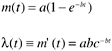
In the model, m(t) is the expected number of failures observed by time t; λ(t) is the failure density; a is the expected number of failures to be observed eventually; and b is the fault detection rate per fault. As seen, m(t) and λ(t) are the cumulative distribution function [F(t)] and the probability density function [f(t)], respectively, of the exponential function discussed in the preceding section. The parameters a and b correspond to K and λ. Therefore, the NHPP model is a straight application of the exponential model. The reason it is called NHPP is perhaps because of the emphasis on the probability distribution of the estimate of the cumulative number of failures at a specific time t, as represented by the first equation. Fitting the model curve from actual data and for projecting the number of faults remaining in the system, is done mainly by means of the mean value, or cumulative distribution function (CDF).
Note that in this model the number of faults to be detected, a, is treated as a random variable whose observed value depends on the test and other environmental factors. This is fundamentally different from models that treat the number of faults to be a fixed unknown constant.
The exponential distribution assumes a pattern of decreasing defect rates or failures. Cases have been observed in which the failure rate first increases and then decreases. Goel (1982) proposed a generalization of the Goel-Okumoto NHPP model by allowing one more parameter in the mean value function and the failure density function. Such a model is called the Goel generalized nonhomogeneous Poisson process model;
where a is the expected number of faults to be eventually detected, and b and c are constants that reflect the quality of testing. This mean value function and failure density function is actually the Weibull distribution, which we discussed in Chapter 7. When the shape parameter m (in the Goel model, it is c) equals 1, the Weibull distribution becomes the exponential distribution; when m is 2, it then becomes the Rayleigh model.
Similar to the NHPP model, in the Musa-Okumoto (M-O) model the observed number of failures by a certain time, τ, is also assumed to be a nonhomogeneous Poisson process (Musa and Okumoto, 1983). However, its mean value function is different. It attempts to consider that later fixes have a smaller effect on the software’s reliability than earlier ones. The logarithmic Poisson process is claimed to be superior for highly nonuniform operational user profiles, where some functions are executed much more frequently than others. Also the process modeled is the number of failures in specified execution-time intervals (instead of calendar time). A systematic approach to convert the results to calendar-time data (Musa et al., 1987) is also provided. The model, therefore, consists of two components—the execution-time component and the calendar-time component.
The mean value function of this model is
where λ is the initial failure intensity, and θ is the rate of reduction in the normalized failure intensity per failure.
With regard to the software defect removal process, Yamada et al. (1983) argue that a testing process consists of not only a defect detection process, but also a defect isolation process. Because of the time needed for failure analysis, significant delay can occur between the time of the first failure observation and the time of reporting. They offer the delayed S-shaped reliability growth model for such a process, in which the observed growth curve of the cumulative number of detected defects is S-shaped. The model is based on the nonhomogeneous Poisson process but with a different mean value function to reflect the delay in failure reporting,
where t is time, λ is the error detection rate, and K is the total number of defects or total cumulative defect rate.
In 1984, Ohba proposed another S-shaped reliability growth model—the inflection S model (Ohba, 1984). The model describes a software failure detection phenomenon with a mutual dependence of detected defects. Specifically, the more failures we detect, the more undetected failures become detectable. This assumption brings a certain realism into software reliability modeling and is a significant improvement over the assumption used by earlier models—the independence of faults in a program. Also based on the nonhomogeneous Poisson process, the model’s mean value function is
where t is time, λ is the error detection rate, i is the inflection factor, and K is the total number of defects or total cumulative defect rate.
The delayed S and inflection S models can be regarded as accounting for the learning period during which testers become familiar with the software at the beginning of a testing period. The learning period is associated with the delayed or inflection patterns as described by the mean value functions. The mean value function (CDF) and the failure density function (PDF) curves of the two models, in comparison with the exponential model, are shown in Figure 8.3. The exponential model assumes that the peak of defect arrival is at the beginning of the system test phase, and continues to decline thereafter; the delayed S model assumes a slightly delayed peak; and the inflection S model assumes a later and sharper peak.
Reliability modeling is an attempt to summarize the complex reality in precise statistical terms. Because the physical process being modeled (the software failure phenomenon) can hardly be expected to be so precise, unambiguous statements of the assumptions are necessary in the development of a model. In applications, the models perform better when the underlying assumptions are met, and vice versa. In other words, the more reasonable the assumptions, the better a model will be. From the preceding summary of several reliability growth models, we can see that earlier models tend to have more restrictive assumptions. More recent models tend to be able to deal with more realistic assumptions. For instance, the J-M model’s five assumptions are:
There are N unknown software faults at the start of testing.
Failures occur randomly—times between failures are independent.
All faults contribute equally to cause a failure.
Fix time is negligible.
Fix is perfect for each failure; there are no new faults introduced during correction.
Together these assumptions are difficult to meet in practical development environments. Although assumption 1 does not seem to pose problems, all the others pose limitations to the model. The Littlewood models, with the concept of error size, overcame the restriction imposed by assumption 3. The Goel-Okumoto imperfect debugging model is an attempt to improve assumptions 4 and 5.
Assumption 2 is used in all time between failures models. It requires that successive failure times be independent of each other. This assumption could be met if successive test cases were chosen randomly. However, the test process is not likely to be random; testing, especially functional testing, is not based on independent test cases. If a critical fault is discovered in a code segment, the tester may intensify the testing of associated code paths and look for other faults. Such activities may mean a shorter time to next failure. Strict adherence to this assumption therefore is not likely. Care should be taken, however, to ensure some degree of independence in data points when using the time between failures models.
The previous assumptions pertain to the time between failures models. In general, assumptions of the time between failures models tend to be more restrictive. Furthermore, time between failures data are more costly to gather and require a higher degree of precision.
The basic assumptions of the fault count model are as follows (Goel, 1985):
Testing intervals are independent of each other.
Testing during intervals is reasonably homogeneous.
Numbers of defects detected during nonoverlapping intervals are independent of each other.
As discussed earlier, the assumption of a homogeneous testing effort is the key to the fault count models. If this assumption is not met, some normalization effort or statistical adjustment should be applied. The other two assumptions are quite reasonable, especially if the model is calendar-time based with wide enough intervals (e.g., weeks).
For both classes of models, the most important underlying assumption is that of effective testing. If the test process is not well planned and test cases are poorly designed, the input data and the model projections will be overly optimistic. If the models are used for comparisons across products, then additional indicators of the effectiveness or coverage of testing should be included for the interpretation of results.
For reliability models, in 1984 a group of experts (Iannino et al., 1984) devised a set of criteria for model assessment and comparison. The criteria are listed as follows, by order of importance as determined by the group:
Predictive validity: The capability of the model to predict failure behavior or the number of defects for a specified time period based on the current data in the model.
Capability: The ability of the model to estimate with satisfactory accuracy quantities needed by software managers, engineers, and users in planning and managing software development projects or controlling change in operational software systems.
Quality of assumptions: The likelihood that the model assumptions can be met, and the assumptions’ plausibility from the viewpoint of logical consistency and software engineering experience.
Applicability: The model’s degree of applicability across different software products (size, structure, functions, etc.).
Simplicity: A model should be simple in three aspects: (1) simple and inexpensive to collect data, (2) simple in concept and does not require extensive mathematical background for software development practitioners to comprehend, and (3) readily implemented by computer programs.
From the practitioner’s point of view and with recent observations of software reliability models, we contend that the most important criteria are predictive validity, simplicity, and quality of assumptions, in that order of importance. Capability and applicability are less significant. As the state of the art is still maturing and striving to improve its most important objective (predictive accuracy), the extra criteria of demanding more functions (capability) for multiple environments (applicability) seems burdensome. Perhaps the accuracy of software reliability models can best be summarized as follows: Some models sometimes give good results, some are almost universally awful, and none can be trusted to be accurate at all times (Brocklehurst and Littlewood, 1992). A model with good predictive validity but poor capability and narrow applicability is certainly superior to one with good capability and wide applicability but with very poor ability to predict.
In contrast to the order of importance determined by the 1984 group, we think that simplicity is much more important, second only to predictive validity. Experts in software reliability models are usually academicians who are well versed in mathematics and statistics. Many modeling concepts and terminologies are outside the discipline of computer science, let alone easy to comprehend and implement by software developers in the industry. As mentioned earlier, some reliability models have not been tested and used in real-life development projects simply because they are not understandable. Simplicity, therefore, is a key element in bridging the gap between the state of the art and the state of practice in software reliability modeling.
The quality of the assumptions is also very important. Early models tend to have restrictive and unrealistic assumptions. More recent models tend to have more realistic assumptions. Better assumptions make the model more convincing and more acceptable by software practitioners; they also lead to better predictive validity.
To model software reliability, the following process or similar procedures should be used.
Examine the data. Study the nature of the data (fault counts versus times between failures), the unit of analysis (CPU hour, calendar day, week, month, etc.), the data tracking system, data reliability, and any relevant aspects of the data. Plot the data points against time in the form of a scatter diagram, analyze the data informally, and gain an insight into the nature of the process being modeled. For example, observe the trend, fluctuations, and any peculiar patterns and try to associate the data patterns with what was happening in the testing process. As another example, sometimes if the unit of time is too granular (e.g., calendar-time in hours of testing), the noise of the data may become too large relative to the underlying system pattern that we try to model. In that case, a larger time unit such as day or week may yield a better model.
Select a model or several models to fit the data based on an understanding of the test process, the data, and the assumptions of the models. The plot in step 1 can provide helpful information for model selection.
Estimate the parameters of the model. Different methods may be required depending on the nature of the data. The statistical techniques (e.g., the maximum likelihood method, the least-squares method, or some other method) and the software tools available for use should be considered.
Obtain the fitted model by substituting the estimates of the parameters into the chosen model. At this stage, you have a specified model for the data set.
Perform a goodness-of-fit test and assess the reasonableness of the model. If the model does not fit, a more reasonable model should be selected with regard to model assumptions and the nature of the data. For example, is the lack of fit due to a few data points that were affected by extraneous factors? Is the time unit too granular so that the noise of the data obscures the underlying trend?
Make reliability predictions based on the fitted model. Assess the reasonableness of the predictions based on other available information—actual performance of a similar product or of a previous release of the same product, subjective assessment by the development team, and so forth.
To illustrate the modeling process with actual data, the following sections give step-by-step details on the example shown in Figures 8.1 and 8.2. Table 8.1 shows the weekly defect rate data.
The data were weekly defect data from the system test, the final phase of the development process. During the test process the software was under formal change con-trol—any defects found are tracked by the electronic problem tracking reports (PTR) and any change to the code must be done through the PTR process, which is enforced by the development support system. Therefore, the data were reliable. The density plot and cumulative plot of the data are shown in Figures 8.1 and 8.2 (ignore temporarily the fitted curves).
Table 8.1. Weekly Defect Arrival Rates and Cumulative Rates
|
Week |
Defects/KLOC Arrival |
Defects/KLOC Cumulative |
|---|---|---|
|
1 |
.353 |
.353 |
|
2 |
.436 |
.789 |
|
3 |
.415 |
1.204 |
|
4 |
.351 |
1.555 |
|
5 |
.380 |
1.935 |
|
6 |
.366 |
2.301 |
|
7 |
.308 |
2.609 |
|
8 |
.254 |
2.863 |
|
9 |
.192 |
3.055 |
|
10 |
.219 |
3.274 |
|
11 |
.202 |
3.476 |
|
12 |
.180 |
3.656 |
|
13 |
.182 |
3.838 |
|
14 |
.110 |
3.948 |
|
15 |
.155 |
4.103 |
|
16 |
.145 |
4.248 |
|
17 |
.221 |
4.469 |
|
18 |
.095 |
4.564 |
|
19 |
.140 |
4.704 |
|
20 |
.126 |
4.830 |
The data indicated an overall decreasing trend (of course, with some noises), therefore the exponential model was chosen. For other products, we had used the delayed S and inflection S models. Also, the assumption of the S models, specifically the delayed reporting of failures due to problem determination and the mutual dependence of defects, seems to describe the development process correctly. However, from the trend of the data we did not observe an increase-then-decrease pattern, so we chose the exponential model. We did try the S models for goodness of fit, but they were not as good as the exponential model in this case.
We used two methods for model estimation. In the first method, we used an SAS program similar to the one shown in Figure 7.5 in Chapter 7, which used a nonlinear regression approach based on the DUD algorithm (Ralston and Jennrich, 1978). The second method relies on the Software Error Tracking Tool (SETT) software developed by Falcetano and Caruso at IBM Kingston (Falcetano and Caruso, 1988). SETT implemented the exponential model and the two S models via the Marquardt non-linear least-squares algorithm. Results of the two methods are very close. From the DUD nonlinear regression methods, we obtained the following values for the two parameters K and λ.
K = 6.597
λ=0.0712
The asymptotic 95% confidence intervals for the two parameters are:
|
Lower |
Upper | |
|---|---|---|
|
K |
5.643 |
7.552 |
|
λ |
0.0553 |
0.0871 |
By fitting the estimated parameters from step 3 into the exponential distribution, we obtained the following specified model
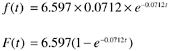
where t is the week number since the start of system test.
We conducted the Kolmogorov-Smirnov goodness-of-fit test (Rohatgi, 1976) between the observed number of defects and the expected number of defects from the model in step 4. The Kolmogorov-Smirnov test is recommended for goodness-of-fit testing for software reliability models (Goel, 1985). The test statistic is as follows:
where n is sample size, F*(x) is the normalized observed cumulative distribution at each time point (normalized means the total is 1), and F(x) is the expected cumulative distribution at each time point, based on the model. In other words, the statistic compares the normalized cumulative distributions of the observed rates and the expected rates from the model at each point, then takes the absolute difference. If the maximum difference, D(n), is less than the established criteria, then the model fits the data adequately.
Table 8.2 shows the calculation of the test. Column (A) is the third column in Table 8.1. Column (B) is the cumulative defect rate from the model. The F*(x) and F(x) columns are the normalization of columns (A) and (B), respectively. The maximum of the last column, |F*(x) − F(x)|, is .02329. The Kolmogorov-Smirnov test statistic for n = 20, and p value = .05 is .294 (Rohatgi, 1976, p. 661, Table 7). Because the D(n) value for our model is .02329, which is less than .294, the test indicates that the model is adequate.
Table 8.2. Weekly Defect Arrival Rates and Cumulative Rates
|
Week |
Observed Defects/KLOC Model Defects/KLOC Cumulative (A) |
Cumulative (B) |
F*(x) |
F(x) |
F*(x) − F(x) |
|---|---|---|---|---|---|
|
1 |
.353 |
.437 |
.07314 |
.09050 |
.01736 |
|
2 |
.789 |
.845 |
.16339 |
.17479 |
.01140 |
|
3 |
1.204 |
1.224 |
.24936 |
.25338 |
.00392 |
|
4 |
1.555 |
1.577 |
.32207 |
.32638 |
.00438 |
|
5 |
1.935 |
1.906 |
.40076 |
.39446 |
.00630 |
|
6 |
2.301 |
2.213 |
.47647 |
.45786 |
.01861 |
|
7 |
2.609 |
2.498 |
.54020 |
.51691 |
.02329 |
|
8 |
2.863 |
2.764 |
.59281 |
.57190 |
.02091 |
|
9 |
3.055 |
3.011 |
.63259 |
.62311 |
.00948 |
|
10 |
3.274 |
3.242 |
.67793 |
.67080 |
.00713 |
|
11 |
3.476 |
3.456 |
.71984 |
.71522 |
.00462 |
|
12 |
3.656 |
3.656 |
.75706 |
.75658 |
.00048 |
|
13 |
3.838 |
3.842 |
.79470 |
.79510 |
.00040 |
|
14 |
3.948 |
4.016 |
.81737 |
.83098 |
.01361 |
|
15 |
4.103 |
4.177 |
.84944 |
.86438 |
.01494 |
|
16 |
4.248 |
4.327 |
.87938 |
.89550 |
.01612 |
|
17 |
4.469 |
4.467 |
.92515 |
.92448 |
.00067 |
|
18 |
4.564 |
4.598 |
.94482 |
.95146 |
.00664 |
|
19 |
4.704 |
4.719 |
.97391 |
.97659 |
.00268 |
|
20 |
4.830 |
4.832 |
1.00000 |
1.00000 |
.00000 |
|
D(n) = .02329 |
We calculated the projected number of defects for the four years following completion of system test. The projection from this model was very close to the estimate from the Rayleigh model and to the actual field defect data.
At IBM Rochester we have been using the reliability modeling techniques for estimating the defect level of software products for some years. We found the Rayleigh, the exponential, and the two S-type models to have good applicability to AS/400’s process and data. We also rely on cross-model reliability to assess the reasonableness of the estimates. Furthermore, historical data are used for model calibration and for adjustment of the estimates. Actual field defect data confirmed the predictive validity of this approach; the differences between actual numbers and estimates are small.
As the example and other cases in the literature illustrate (for example, Misra, 1983; Putnam and Myers, 1992), a fair degree of accuracy to project the remaining number of defects can be achieved by software reliability models, based on testing data. This approach works especially well if the project is large, where defect arrivals tend not to fluctuate much; if the system is not for safety-critical missions; and if environment-specific factors are taken into account when choosing a model. For safety-critical systems, the requirements for reliability and, therefore, for reliability models, are much more stringent.
Even though the projection of the total number of defects (or defect rates) may be reasonably accurate, it does not mean that one can extend the model density curve from the testing phase to the maintenance phase (customer usage) directly. The defect arrival patterns of the two phases may be quite different, especially for commercial projects. During testing the sole purpose is to find and remove defects; test cases are maximized for defect detection, therefore, the number of defect arrivals during testing is usually higher. In contrast, in customers’ applications it takes time to encounter defects—when the applications hit usual scenarios. Therefore, defect arrivals may tend to spread. Such a difference between testing-defect density and field-defect density is called the compression factor. The value of the compression factor varies, depending on the testing environments and the customer usage profiles. It is expected to be larger when the test strategy is based on partition and limit testing and smaller for random testing or customer-environment testing. In the assessment by Elbert and associates (1992) on three large-scale commercial projects, the com-pression factor was 5 for two projects and 30 for a third. For projects that have extensive customer beta tests, models based on the beta test data may be able to extrapolate to the field use phase.
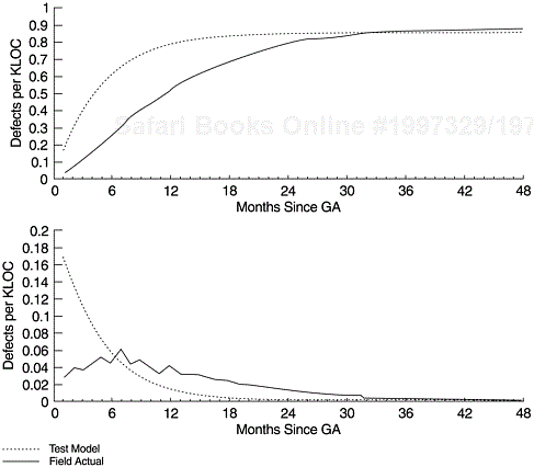
Figure 8.4 shows a real-life example of compression of defect density between testing and initial data from the field. For the upper panel, the upper curve represents the extrapolated cumulative defect rate based on testing data. The lower curve is the actual cumulative field defect rate. Although the points of the two curves at four years in the life of product are close, the upper curve has a much faster buildup rate. The difference is even more drastic in the lower panel, in which the two defect density curves are contrasted. The extrapolated curve based on testing data is front loaded and declines much faster. In vivid contrast, the actual field defect arrival is much more spread out. It even follows a different density pattern (a delayed S or a Rayleigh-like pattern).
Based on the discussions in the previous section, it is apparent that for software maintenance planning, we should (1) use the reliability models to estimate the total number of defects or defect rate only and (2) spread the total number of defects into arrival pattern over time based on historical patterns of field defect arrivals.
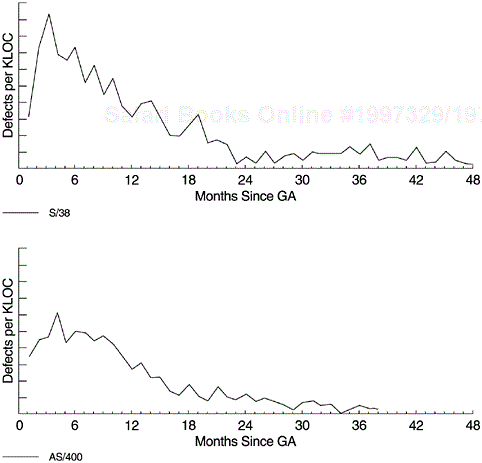
The field defect arrival patterns, in turn, can be modeled by the same process. Our experience with several operating systems indicates that the arrival curves follow the Rayleigh, the exponential, or the S models. Figure 8.5 shows the field defect arrival patterns of a major release of both the System/38 and the AS/400 operating systems. As discussed in Chapter 7, Figure 7.6 shows the field defect arrivals pattern of another IBM system software, which can be modeled by the Rayleigh curve or the Weibull distribution with the shape parameter, m, equal to 1.8.
The field defect arrival pattern may differ for different types of software. For example, in software for large systems it takes longer for latent defects to be detected and reported. The life of field defect arrivals can be longer than three years. For applications software, the arrival distribution is more concentrated and usually last about two years. We call the former the slow ramp-up pattern and the latter the fast ramp-up pattern. Based on a number of products for each category, we derived the distribution curves for both patterns, as shown in Figure 8.6. The areas under the two curves are the same, 100%. Tables 8.3 and 8.4 show the percent distribution by month for the two patterns. Because the defect arrival distribution pattern may depend on the type of software and industry segment, one should establish one’s own pattern based on historical data. If the defect arrival patterns cannot be modeled by a known reliability model, we recommend using a nonparametric method (e.g., 3-point moving average) to smooth the historical data to reveal a pattern and then calculate the percent distribution over time.
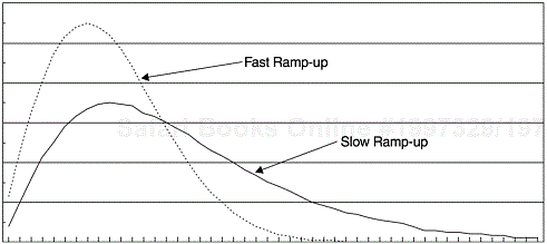
Table 8.3. Monthly Percent Distribution of Field Defect Arrivals—Slow Ramp-up Pattern
|
Month |
% |
Month |
% |
Month |
% |
Month |
% |
|---|---|---|---|---|---|---|---|
|
1 |
0.554 |
13 |
4.505 |
25 |
1.940 |
37 |
0.554 |
|
2 |
1.317 |
14 |
4.366 |
26 |
1.802 |
38 |
0.416 |
|
3 |
2.148 |
15 |
4.158 |
27 |
1.594 |
39 |
0.416 |
|
4 |
2.911 |
16 |
3.950 |
28 |
1.386 |
40 |
0.347 |
|
5 |
3.465 |
17 |
3.742 |
29 |
1.247 |
41 |
0.347 |
|
6 |
4.019 |
18 |
3.465 |
30 |
1.178 |
42 |
0.277 |
|
7 |
4.366 |
19 |
3.188 |
31 |
1.040 |
43 |
0.277 |
|
8 |
4.643 |
20 |
2.980 |
32 |
0.970 |
44 |
0.208 |
|
9 |
4.782 |
21 |
2.772 |
33 |
0.832 |
45 |
0.208 |
|
10 |
4.851 |
22 |
2.495 |
34 |
0.762 |
46 |
0.138 |
|
11 |
4.782 |
23 |
2.287 |
35 |
0.693 |
47 |
0.138 |
|
12 |
4.712 |
24 |
2.079 |
36 |
0.624 |
48 |
0.069 |
|
Year 1 |
42.550 |
Year 2 |
82.537 |
Year 3 |
96.605 |
Year 4 | |
|
Cumulative |
Cumulative |
Cumulative |
Cumulative |
100.000 |
Table 8.4. Monthly Percent Distribution of Field Defect Arrivals—Fast Ramp-up Pattern
|
Month |
% |
Month |
% Month |
% | |
|---|---|---|---|---|---|
|
1 |
1.592 |
13 |
5.398 |
25 |
0.277 |
|
2 |
3.045 |
14 |
4.706 |
26 |
0.208 |
|
3 |
4.429 |
15 |
4.014 |
27 |
0.128 |
|
4 |
5.536 |
16 |
3.391 |
28 |
0.069 |
|
5 |
6.505 |
17 |
2.768 |
29 |
0.069 |
|
6 |
7.128 |
18 |
2.215 |
30 |
0.069 |
|
7 |
7.474 |
19 |
1.730 | ||
|
8 |
7.612 |
20 |
1.384 | ||
|
9 |
7.474 |
21 |
1.038 | ||
|
10 |
7.197 |
22 |
0.761 | ||
|
11 |
6.713 |
23 |
0.554 | ||
|
12 |
6.090 |
24 |
0.415 | ||
|
Year 1 |
70.795 |
Year 2 |
99.169 |
Year 2.5 |
99.999 |
|
Cumulative |
Cumulative |
Cumulative |
The exponential distribution, another special case of the Weibull distribution family, is the simplest and perhaps most widely used distribution in reliability and survival studies. In software, it is best used for modeling the defect arrival pattern at the back end of the development process—for example, the final test phase. When calendar-time (versus execution-time) data are used, a key assumption for the exponential model is that the testing effort is homogeneous throughout the testing phase. If this assumption is not met, normalization of the data with respect to test effort is needed for the model to work well.
In addition to the exponential model, numerous software reliability growth models have been proposed, each with its own assumptions, applicability, and limitations. However, relatively few have been verified in practical environments with industry data, and even fewer are in use. Based on the criteria variable they use, software reliability growth models can be classified into two major classes: time between failures models and fault count models. In this chapter we summarize several well-known models in each class and illustrate the modeling process with a real-life example. From the practitioner’s vantage point, the most important criteria for evaluating and choosing software reliability growth models are predictive validity, simplicity, and quality of assumptions.
Software reliability models are most often used for reliability projection when development work is complete and before the software is shipped to customers. They can also be used to model the failure pattern or the defect arrival pattern in the field and thereby provide valuable input to maintenance planning.