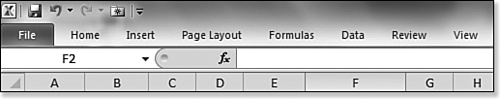
2. The Ribbon Interface and Quick Access Toolbar
If you have upgraded directly to Excel 2010 from Excel 2003 or earlier, you are going through the shock of discovering that the familiar File, Edit, View, Insert, Format, Tools, Data, Window, and Help menus, along with the Standard and Formatting toolbars, are gone from Excel 2010.
In their place, Microsoft introduces the Ribbon.
Using the Ribbon
The Ribbon is composed of seven permanent tabs labeled Home, Insert, Page Layout, Formulas, Data, Review, and View.
Each tab is broken into rectangular groups of related commands. The group shown in Figure 2.1 is the Clipboard group.
Figure 2.1. Detail of the Clipboard group of the Home tab of the Ribbon.
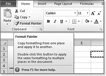
The mantra of the Ribbon is to use Pictures and Words. Many people have seen the little Whisk Broom icon in previous versions of Office but never knew what it did. If you hover over the icon in Excel 2003, the ToolTip tells you that it was the Format Painter, which at least gave you a place to start looking in the Help file if you were really curious.
In Excel 2010, the same icon has the words “Format Painter” next to the icon. When you hover, the ToolTip offers paragraphs explaining what the tool does. The ToolTip offers a little-known trick: You can double-click the Format Painter to copy the formatting to many places. The ToolTip offers a link to the help topic about the Format Painter. All these steps are designed to help more people find and make use of the Format Painter tool.
In Figure 2.1, the Cut icon is a pure command. You click the icon and Excel cuts the selection onto the Clipboard.
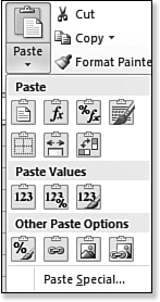
In contrast, the Paste and Copy icons are a new type of element in that each represents a hybrid command. Figure 2.2 is shot with the mouse pointer hovering over the Paste icon. You see that this icon is actually two icons. The top half of the icon is the actual Paste command. The bottom half of the icon is a drop-down menu offering other types of Paste commands (see Figure 2.3).
Figure 2.2. The Paste icon is actually two icons; a Paste command and a Paste drop-down.
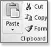
Figure 2.3. Click the bottom of the Paste icon to access more paste options.
Using Dialog Launchers and the 80/20 Rule
The Ribbon is designed to make it easier to discover features that should be used by most people using Excel. It is not designed to hold every command available in Microsoft Excel. In many cases, even the middle-of-the-road Exceller needs to go beyond the commands on the Ribbon.
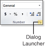
A special symbol in the lower-right corner of many Ribbon groups takes you directly to the dialog box with many more choices than those offered in the Ribbon.
Figure 2.4 shows detail of the Number group of the Home tab. In the lower-right corner is a tiny symbol. The symbol is the top-left corner of a box, with an arrow pointing downward to the right. This symbol is called a dialog launcher.
Figure 2.4. The dialog launcher takes you to additional options.
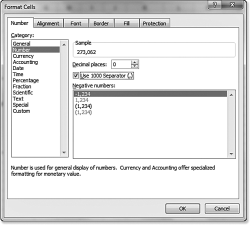
When you click the dialog launcher, you go to a dialog box that often offers many more choices than those available in the Ribbon. In Figure 2.5, you see the Number tab of the Format Cells dialog.
Figure 2.5. Click the dialog launcher to get to the full dialog box with all the choices.
Dialog launchers are not the only way to access dialog boxes. Flyout menus and galleries offer their own way to reach dialog boxes.
Using Flyout Menus and Galleries
The Ribbon introduces two new kinds of controls; visual flyout menus and galleries.
Figure 2.6 shows the visual flyout menu that appears when you open the Conditional Formatting drop-down on the Home tab. You can see that the initial menu continues to offer pictures and words, with words next to the icons for Data Bars, Color Scales, and Icon Sets. When you hover over a selection, a flyout menu appears with more visual choices (see Figure 2.6).
Figure 2.6. The flyout menus continue the theme of offering pictures and words.
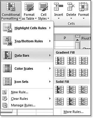
Note the More Rules option at the bottom of the Data Bars menu. The More command occurs at the bottom of many flyout menus. When you see More, you will know that the menu is offering you only a subset of options. Click More to access all the options.
Another new element in the Ribbon is the gallery control. Galleries are used when there are dozens of options from which to choose. The gallery shows you a visual thumbnail of each choice.
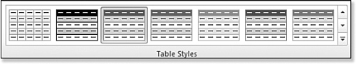
In Figure 2.7, you see the first row of choices in the Table Styles gallery. Notice the three arrows at the right end of the gallery.
Figure 2.7. A gallery control starts by showing one row of thumbnails but offers three arrow controls at the right end.
You can use the up-arrow and down-arrow icons to browse through the gallery one row at a time. Or you can press the third arrow to open the entire gallery and see all the choices, as shown in Figure 2.8.
Figure 2.8. If you open the gallery control, you can scroll through more choices.
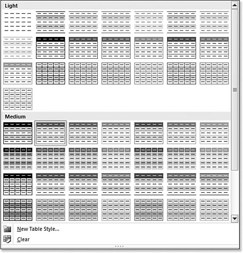
Again, at the bottom of Figure 2.8, you have additional choices for New Table Style. This leads to a dialog box with all the options around table styles.
The Ribbon Is Constantly Changing
Although you start out with Ribbon tabs for File, Home, Insert, Page Layout, Formulas, Data, Review, and View, you constantly see other tabs appearing and disappearing. Further, as you resize your Excel window, the icons change and resize.
Harnessing Contextual Ribbon Tabs
Excel 2010 offers a whole series of commands for dealing with photographs that you insert into your worksheet. However, 90% of the people never bother to dress up their worksheets with clip art or pictures, so there really is no reason to show all the commands for working with photographs in the Ribbon.
There is one persistent command in the Ribbon that deals with pictures. You can use the Picture command on the Insert tab of the Ribbon to insert a picture.
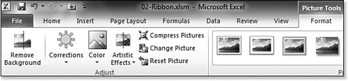
After you use that command to insert a picture, and provided that the picture is selected, a new tab called Picture Tools Format appears. This tab offers a gallery with all sorts of tools for changing the appearance of the picture. See Figure 2.9 for some detail from the Picture Tools Format tab.
Figure 2.9. When a picture is selected, the Picture Tools Format tab is available.
Here is the frustrating thing. As soon as you click outside of the picture, the picture is no longer selected and the Picture Tools Format tab disappears.
If you need to format an object and you cannot find the icons for formatting the object, try clicking the object to see if the contextual tabs appear.
These are the context-sensitive tabs:
• Add-Ins—This tab contains any menu items added through VBA macros or add-ins. This tab appears when an add-in is loaded.
• Background Removal—This tab is new in Excel 2010 and is used to remove the background from a photograph. To access the tab, use the Background Removal icon on the Picture Tools tab.
• Chart Tools—The Chart Tools tab includes three tabs: Design, Layout, and Format. The Design tab provides features to change an entire chart. By the time you get to the Format tab, you are micromanaging small aspects of a chart.
• Drawing Tools—This includes a Format tab for working with shapes. To access the tab, select Insert, Shapes.
• Equation Tools—The Design tab appears when you use the Equation Editor.
• Header & Footer—This tab appears when you edit the header or footer for a page in Page Layout view. To access the tab, you click View, Page Layout View and then click in either the header or footer zone. Note that there is a shortcut to Page Layout View, located to the left of the zoom slider, in the lower-right corner of the screen.
• Ink Tools—This tab contains Pens commands for tablet PCs.
• Picture Tools—This tab is available after you insert clip art or an image and select the illustration.
• Pivot Chart Tools—After you insert a pivot chart, four new tabs are available: Design, Layout, Format, and Analyze. The first three of these tabs are similar to the Chart Tools tabs. The fourth contains the pivot table features.
• PivotTable Tools—This includes two tabs: Options and Design. The major settings appear on the Options tab. Formatting options appear on the Design tab.
• Print Preview Tools—This small tab appears as the only tab when you are in Print Preview mode. Because Print Preview moved to the Backstage view, this tab will be very elusive.
• Slicer Tools—The Options tab appears whenever one of the new Excel 2010 visual filters for pivot tables is selected.
• SmartArt Tools—In Excel 2010, the former business diagrams has been renamed SmartArt. When you are working with organization charts or other SmartArt diagrams, two new tabs are available: Design and Format.
• Sparkline Tools—The Design tab appears whenever the current selection is in a sparkline. Sparklines are tiny, word-sized charts that debuted in Excel 2010.
• Table Tools—The Design tab allows for the formatting of a database in Excel after it has been converted to a table. In Excel 2010, tables replace Excel 2003 lists.
All these contextual tabs come and go as you select and clear certain items in Excel.
Resizing Excel Changes the Ribbon
You need a monitor with a 1440-pixel-wide resolution to see the entirety of the Ribbon. Anytime that you view the Ribbon at a smaller size, Excel starts intelligently collapsing icons on the Ribbon.
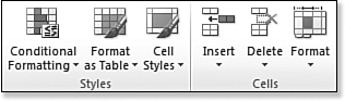
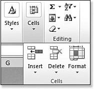
Figure 2.10 shows the Styles and the Cells group of the Home tab at a 1280 resolution. At this resolution, the Cell Styles gallery visible at 1440 resolution has already collapsed into a large drop-down icon.
Figure 2.10. At 1280 resolution, the Styles and Cells groups appear as six large drop-down icons.
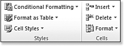
At a smaller resolution, the size of the six icons gets smaller, but you still have words, as shown in Figure 2.11.
Figure 2.11. At smaller resolutions, the icons shrink.
Eventually, those groups shrink into a single drop-down for the entire group, as shown in Figure 2.12.
Figure 2.12. Eventually, the entire group collapses to a single drop-down.
If you continue to shrink the width of the Excel window, the Ribbon disappears altogether, as shown in Figure 2.13.
Figure 2.13. Below 300 pixels of width, Microsoft figures that you are not working in the application anymore and hides the Ribbon entirely.
![]() To see the Ribbon changing when the window is resized, search for Excel In Depth 2 at YouTube.
To see the Ribbon changing when the window is resized, search for Excel In Depth 2 at YouTube.
Solving Common Ribbon Problems
Here are some common complaints about the Ribbon and some advice on how to best deal with these issues.
You Cannot Find a Particular Command on the Ribbon
Here are some tips for working with the Ribbon:
• Start on the Home tab. All the commands on the old Formatting toolbar are here, as well as most of the old Insert and Format menus.
• Pivot tables moved from the Data tab to the Insert tab. They don’t belong here. They belong on the Data tab with all the other commands from the old Data menu.
• The four most popular commands on the Excel 2003 Insert menu are no longer on the Insert tab. Insert Cells, Insert Rows, Insert Columns, and Insert Worksheet are all now found under the Insert drop-down in the Cells group of the Home tab.
• Commands from the old Tools menu are generally found on the Review tab.
• Commands from the old Window menu are generally found on the View tab.
• Macro commands are on a Developer tab of the Ribbon that is hidden by default. See Chapter 4, “Customizing the Ribbon,” for how to bring the Developer tab back.
You Still Cannot Find the Command on the Ribbon
Following are many strategies for finding the command:
• If you remember the old Excel 2003 keyboard accelerators, try typing those. For example, Alt+E+I+J still invokes Edit, Fill, Justify, even though there is no longer an Edit tab on the Ribbon.
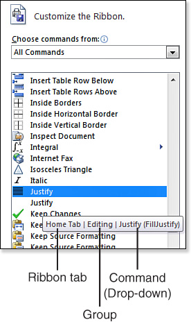
• Right-click the Ribbon and select Customize. In the Customize dialog, select All Commands from the left drop-down. Scroll through the list of all commands until you find the command. Hover over the command. A ToolTip appears, showing you where you can find the command. In Figure 2.14, the Justify command is located on the Home tab, in the Editing Group, under the Fill drop-down.
Figure 2.14. This ToolTip in the Customize dialog shows you where to find a command.
• Download my full-color tip card that maps every old command in the Excel 2003 menu and toolbars to a Ribbon tab. You can access the tip card at http://www.mrexcel.com/excel2007tipcard.html.
• Microsoft has an interactive Ribbon guide that can help you locate an Excel 2003 menu command on the Ribbon. Type Interactive Ribbon guide in any search engine to find the latest incarnation of the Ribbon guide.
Note
![]()
Sometimes, a command truly is not in the Ribbon. If you hover over a command in the Customize dialog and it indicates that it is a command that is not in the Ribbon, you will have to use Customize to add this command to the Quick Access Toolbar or to the Ribbon.
The Ribbon Takes Up Too Many Rows
I don’t want to argue with you, but the new Ribbon only appears to take up a lot of space. It does not take up more space than the Excel 2003 menu, formatting, and standard toolbars (provided you showed those toolbars on two rows).
However, you can minimize the Ribbon using one of these techniques:
Click the Caret icon on the right side of the Ribbon, just to the left of help (see Figure 2.15).
Figure 2.15. Caret icon to minimize the Ribbon.
Right-click the Ribbon and select Minimize the Ribbon.
When the Ribbon is minimized, you see only the words Home, Insert, Page Layout, and so on (see Figure 2.16). After you click a tab, the Ribbon temporarily reappears. When you finish selecting a command, the Ribbon goes back to the minimized size.
Figure 2.16. When the Ribbon is minimized, you see only the tab names.
You Do Not Like Where Something Is Located on the Ribbon
I am with you on this one. Pivot Tables belong on the Data tab, not on the Insert tab. Further, if you could take the left half of the Home tab and combine it with the right half of the Data tab, most people would hardly ever have to leave that one tab.
The great news in Excel 2010 is that you can now customize the Ribbon.
![]() See Chapter 4 to learn more about customizing the Ribbon.
See Chapter 4 to learn more about customizing the Ribbon.
You Cannot See All Your Favorite Commands at Once
A problem with the Ribbon is that only one-seventh of the commands are visible at any given time. You will find yourself moving from one tab to another. The alternative is to use the Quick Access Toolbar.
Using the Quick Access Toolbar
The Quick Access Toolbar is a customizable toolbar. It remains visible, no matter which tab is currently displayed. Because the Quick Access Toolbar is always visible, you can store your most used commands and have them always visible.
There are probably a handful of toolbar buttons that you use constantly. For me, the list would be Sort Ascending, Print, Filter by Selection, Align Right, Open Recent Files, and Decrease Decimal. If you tried to locate these five commands, you would find that they are spread throughout the Ribbon interface.
Luckily, the Quick Access Toolbar comes to the rescue. The Quick Access Toolbar holds up to 90 of your favorite icons. It is always visible on the screen, so you can access its icons without needing to change to a different tab.
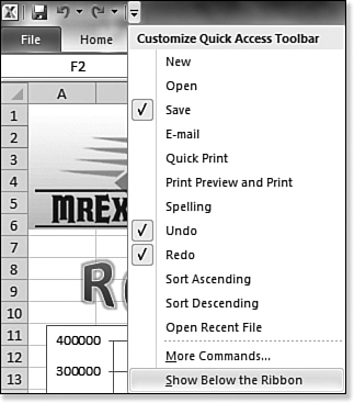
Changing the Location of the Quick Access Toolbar
The Quick Access Toolbar is initially displayed above the left side of the ribbon. Initially, the menu offers Save, Undo, Redo, and Quick Print icons. Figure 2.17 shows the initial location and configuration of the Quick Access Toolbar.
Figure 2.17. The default location of the Quick Access Toolbar is above the Ribbon.
The other option is to display the Quick Access Toolbar immediately below the Ribbon. To do so, click the drop-down arrow at the right edge of the Quick Access Toolbar. Then select Show Below the Ribbon, as shown in Figure 2.18.
Figure 2.18. You can move the Quick Access Toolbar below the Ribbon.
When the Quick Access Toolbar is below the Ribbon, you can use a similar method to move the Quick Access Toolbar back above the Ribbon: Click the drop-down on the right side of the Quick Access Toolbar and select Show Above the Ribbon.
Adding Favorite Commands to the Quick Access Toolbar
The drop-down shown in Figure 2.18 offers 12 popular commands that you might choose to add to the Quick Access Toolbar. Of my six desired icons, three are already available in that list.
When you find a command in the Ribbon that you are likely to use often, you can add the command to the Quick Access Toolbar. To do so, right-click any command in the Ribbon and select Add to Quick Access Toolbar. For example, to add Align Right to the Quick Access Toolbar, follow these steps:
- Access the Home tab.
- Right-click the Align Right icon.
- Select Add to Quick Access Toolbar.
Items added to the Quick Access Toolbar using the right-click method are added to the right side of the Quick Access Toolbar.
Knowing Which Commands Can Be on the Quick Access Toolbar
You can add commands to the Quick Access Toolbar, but you cannot add the contents of many lists on the Ribbon. Figuring out what you can and cannot add to the Quick Access Toolbar requires a bit of experimentation.
For example, consider the Orientation icon in the Alignment group of the Home tab. You can use this icon to angle text counterclockwise. The icon also contains a drop-down that has a total of six commands: Angle Counterclockwise, Angle Clockwise, Vertical Text, Rotate Text Up, Rotate Text Down, and Alignment. If you right-click the Alignment icon and choose to add it to the Quick Access Toolbar, the entire icon, along with the drop-down of six commands, is added.
If you don’t want to add the entire drop-down to the Quick Access Toolbar, you can instead open the drop-down and right-click one of the six items. Just this individual command is added to the Quick Access Toolbar.
However, other drop-downs are not drop-downs of commands. Instead, they may lead to drop-downs with list boxes. For example, consider the font size drop-down. It is possible to add the entire font size drop-down as an icon on the Quick Access Toolbar, but it is not possible to add to the Quick Access Toolbar individual items from the list. You can add the drop-down itself, but you cannot, for example, add to the Quick Access Toolbar an item that changes the font to 16 points.
If you right-click an item in a list and the context menu doesn’t offer the ability to add it to the Quick Access Toolbar, this is probably not a real command.
Removing Commands from the Quick Access Toolbar
You can remove an icon from the Quick Access Toolbar by right-clicking the icon and selecting Remove from Quick Access Toolbar.
You can also remove icons by using the Excel Options dialog, as discussed in the following section.
Customizing the Quick Access Toolbar
You can make minor changes to the Quick Access Toolbar by using the context menus, but you can have far more control over the Quick Access Toolbar if you use the Customize command. You right-click the Quick Access Toolbar and select Customize Quick Access Toolbar to display the Quick Access Toolbar section of the Excel Options dialog, as shown in Figure 2.19.
Figure 2.19. You can completely customize the Quick Access Toolbar using the Excel Options dialog.

The Excel Options dialog offers many features for customizing the Quick Access Toolbar:
You can choose to customize the Quick Access Toolbar for all documents on your computer or just for the current document.
You can add separators between icons to group the icons logically.
You can resequence the order of the icons on the toolbar.
You can access 1,286 commands, including the commands from every tab and commands that are not available in the Ribbon.
You can reset the Quick Access Toolbar to its original default state.
You can move the Quick Access Toolbar to appear above or below the Ribbon.
Using the Excel Options to Customize the Quick Access Toolbar for All Workbooks
In the default state, the Customize Quick Access Toolbar drop-down in the Excel Options dialog is set to For All Documents (Default). This means that any changes you make to the Quick Access Toolbar will apply to all Excel documents opened on this computer.
Initially, the Choose Commands From drop-down shows Popular commands. This drop-down lists every tab, plus two useful selections. If you select All Commands, you get an alphabetical list of every possible command. If you select Commands Not in the Ribbon, you see only the commands that you might have used in Excel 2003, but did not make it to a tab.
To add a new icon to the Quick Access Toolbar for all workbooks, follow these steps:
- Choose the proper command subset from the Choose Commands From drop-down.
- Select the icon in the Choose Commands From list box. You might have to scroll to see the complete list.
- Click the Add button to add the command to the Customize Quick Access Toolbar.
The top choice in each category is a value called <Separator>. You can add this to the Customize Quick Access Toolbar list to create a vertical bar between icons on the Quick Access Toolbar.
Customizing Icons for the Current Workbook Only
Suppose you have 10 icons on your Quick Access Toolbar for all workbooks. If you add additional icons for this workbook only, the icons appear after the 10 icons for all workbooks. To add these additional icons, follow these steps.
- Right-click the Quick Access Toolbar or most places in the Ribbon and select Customize Quick Access Toolbar.
- With the Customize Quick Access Toolbar drop-down set to For All Documents, select the <Separator> icon at the top of the Choose Commands From list box. Click Add to add a vertical line at the end of the “all workbooks” section of the Quick Access Toolbar.
- From the Customize Quick Access Toolbar drop-down, select For (This Workbook Name).
- Use the Choose Commands From drop-down to find particular categories.
- Select an icon in the Customize Quick Access Toolbar list.
- Click the Add button.
- Repeat steps 4–6 as needed.
- Click OK to complete the operation.
When you finish with this process, the Quick Access Toolbar shows the icons that apply to all workbooks, a vertical separator, and then icons that apply only to the current workbook.
Tip
![]()
If you are going to use icons for all workbooks and additional icons for this workbook only, you might want to end the workbook icons with a separator to help identify where the icons for this workbook only begin.
If you have the current workbook open and then switch to another open workbook, the icons assigned to the current workbook are hidden. If you arrange the windows so that you can see many workbooks at the same time, the icons for the current workbook stay visible as long as the workbook is active.
Filling Up the Quick Access Toolbar
The Quick Access Toolbar allows about 90 icons and/or separators. This is more than will fit across the screen on most monitors. If the monitor is not large enough to display all the icons, the first 54 of them are shown onscreen, and the rest are hidden behind a double arrow at the right edge of the Quick Access Toolbar.
Rearranging Icons on the Quick Access Toolbar
You can rearrange icons on the Quick Access Toolbar by using the Excel Options dialog. Select any icon from the Customize Quick Access Toolbar list box and then use the up-arrow or down-arrow buttons on the far right side of the dialog to move the icon up or down.
Resetting the Quick Access Toolbar
If you start a new job and inherit someone else’s computer, you might want to start with a fresh slate of icons on the Quick Access Toolbar. To reset the Quick Access Toolbar to the default configuration, follow these steps:
- With the Customize Quick Access Toolbar drop-down set to For All Documents (Default), click the Reset button at the bottom of the Customize Quick Access Toolbar list box. A warning box asks if you want to reset the list for all workbooks.
- Click OK, and the list returns to the three default icons (Save, Undo, and Repeat).
- With the Customize Quick Access Toolbar drop-down set to For (This Workbook), click the Reset button at the bottom of the Customize Quick Access Toolbar list box. A warning box asks if you want to reset the list for this particular document.
- Click OK, and the list clears.
Note
![]()
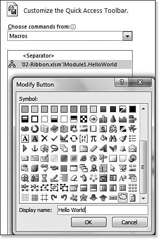
I am not sure why you would choose to use the Print icon for your macros. Considering that you used to have 4,096 choices and now have only 180 choices, this is another area where Excel 2010 does not live up to the legacy versions.
Assigning VBA Macros to Quick Access Toolbar Buttons
Typically, a VBA macro is assigned to a shortcut key. In legacy versions of Excel, it was easy to customize the menu system to add commands to invoke macros. In legacy versions of Excel, more than 4,000 different icons were available for the various custom menu items.
Excel 2010 offers a weak interface for adding custom macros to the Quick Access Toolbar. In the Excel Options dialog is a drop-down called Macros. If you select this group, you see all public macros in all open workbooks. You can select a macro and click Add to add that macro to the Quick Access Toolbar.
Initially, every macro added to the Quick Access Toolbar gets an identical icon. However, you can select an icon in the Customize Quick Access Toolbar list box and click the Modify button. The Modify Button dialog box that appears allows you to choose from 55 available icons for a macro. Most of these buttons are similar to icons that are already popular. For example, the Print icon is fairly well known and has a meaning. In addition to choosing from the 55 icons, you can type any text for a display name, as shown in Figure 2.20. The display name does not appear next to the button. But if you hover your mouse over the icon on the Quick Access Toolbar, you can see the display name in a ToolTip.
Figure 2.20. For macros, you can customize the button image and add a display name on the Quick Access Toolbar.