18. Using Names in Excel
Long before Microsoft introduced tables and formulas like =[@Revenue]–[@ Cost], spreadsheets have offered the ability to assign a name to a cell, range of cells, or formula. The theory is that using a name for a range would be easier to understand when used in a formula. =SUM(MyExpenses) would make formulas more self-documenting than =SUM(Sheet5!AB2:AB99). In Excel 2010, you use the Name Manager interface to assign and use names effectively.
Use the Name Box to Define a Name for a Cell
There are a variety of uses for names in a workbook. A name can be applied to any cell or range. Names are also useful for the following:
• Making formulas easier to understand
• Quick navigation
• Forcing a formula reference to remain absolute, without having to use the dollar sign
• Improving Solver’s report results
• Storing a value that will be used repeatedly, but that might occasionally need to change such as a sales tax rate
• Storing formulas
• Defining a dynamic range
Note
![]()
Excel 2010 offers the new Table functionality, which is described in Chapter 19, “Fabulous Table Intelligence.” Although the Table feature allows you to create formulas using column names, the individual column names and table name are not considered named ranges.
There are various ways to name a cell. The easiest way to define a name for a cell is to use the Name box. To do so, select any cell in your worksheet. To the left of the formula bar is a box with the address of that cell. This box is known as the Name box (see Figure 18.1). The quick way to assign a name is to click inside the Name box and type a name, such as Revenue.
Figure 18.1. The Name box is to the left of the formula bar.
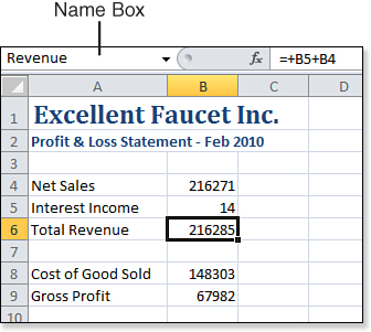
When you press Enter, Excel centers the name in the Name box, which indicates that the name has been assigned. This is your only indication that the name is valid and has been accepted.
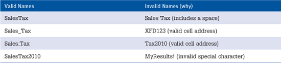
The following are some basic rules for valid names:
• Names can be up to 255 characters long.
• Names cannot contain spaces. However, you can use an underscore or a period in a name. For example, the names Gross_Profit and Gross.Profit are valid.
• Names cannot look like cell addresses.
• Names cannot contain operator characters such as these: +-*/()^&<>=%.
• Names cannot contain special characters such as !“#$’,;:@[]{}`|~.
Table 18.1 provides some examples of valid and invalid names.
Table 18.1. Examples of Valid and Invalid Names
Naming a Cell by Using the Name Dialog
The Formulas tab contains a group called Defined Names. The following example introduces the Name dialog:
- Select a cell that you would like to name. Click the Define Name icon from the Formulas tab. The New Name dialog box appears. In Figure 18.2, Cell B8 is being assigned a name.
Figure 18.2. Choose a cell to be named and then select Define Name from the Formulas tab.
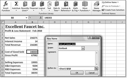
- The New Name box uses IntelliSense to propose a name. Notice that in this particular example, Excel’s IntelliSense was able to ascertain that this cell contains the text Cost of Good Sold. Because that is not a valid name, Excel instead proposed naming the cell Cost_of_Good_Sold. You can either keep that name or override it with a name that you prefer. In this case, override that name with the name COGS.
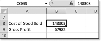
As you can see in Figure 18.3, the name was applied because the Name box now shows COGS instead of B8.
Figure 18.3. After you assign a name, the Name box reflects the new name.
Using the Name Box for Quick Navigation
One advantage of using names is that you can use the drop-down in the Name box to jump to any named cell. This includes cells that might be in distant sections of the worksheet or even on other sheets in the workbook.
If you plan to use the Name box for navigation, assign a name to the upper-left corner of each section of your workbook. The Name box drop-down will then provide a minitable of contents, and people can use the Name box to jump to any section of the workbook.
To illustrate this concept, follow these steps:
- Click the New Sheet icon (next to the right-most sheet tab) to add a new sheet to the workbook.
- On the new sheet, go to a distant cell. Give that cell a name, such as SectionTwo. Return to the original sheet in the workbook.
- Click the Name box’s drop-down arrow to access a list of all names in the workbook, as shown in Figure 18.4.
Figure 18.4. The Name Box drop-down contains a list of all names in the workbook.
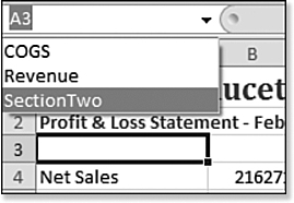
- Choose a name from the list to navigate quickly to that cell, even if it is on another worksheet.
As you can see, named ranges are a great tool for quickly navigating a workbook. Note that names are presented in the Name box alphabetically. If you want the names to appear sequentially, you can add names such as Section1, Section2, Section3, and so on. You can also prefix the section names with letters such as A-Income, B-Costs, C-Expense, D-Tax, E-Income. Then, you can jump to a section by choosing it from the alphabetical list in the Name box. When used in this way, names in Excel are almost like bookmarks in Word.
Using Scope to Allow Duplicate Names in a Workbook
Ideally, you should keep the names unique throughout a workbook. Although it is technically legal to add a name such as SectionOne to both Sheet1 and Sheet2, it is not a good idea. When you define the name on the first sheet, it is defined as a name with workbook-level scope. This means that you can easily navigate to SectionOne from any sheet in the workbook. If you attempt to set up the same name on a second worksheet, that name will have to be set up with worksheet-level scope. Names with worksheet-level scope override the workbook-level scope only on the sheets on which they are defined. For example, suppose you have a workbook with Sheet1, Sheet2, Sheet3, Sheet4, and Sheet5:
• On Sheet2, you use the Name box to assign the name SectionOne to Cell N16.
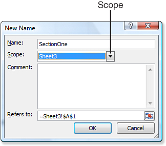
• On Sheet3, you use the New Name dialog to assign the name SectionOne to Cell A1. In the New Name dialog, you need to change the Scope setting from Workbook to Sheet3, as shown in Figure 18.5
Figure 18.5. Change the scope of the duplicate name to apply only on Sheet3.
• If you are on Sheet3 and use the Name box to navigate to SectionOne, you will jump to Cell A1 on Sheet3.
• If you are on any other sheet in the workbook and use the Name box to navigate to SectionOne, you will jump to Cell N16 on Sheet2.
Note
![]()
The names Print_Area and Print_Titles are common worksheet-level names. These names are assigned by Excel after you set certain print settings.
You can see that this can be confusing. In general, you should stick with unique names that can have workbook-level scope. You should switch to using duplicate names with worksheet-level scope only when you have many nearly identical sheets in a workbook.
Using Named Ranges to Simplify Formulas
As introduced at the start of this chapter, the original reason for having named ranges was to simplify formulas. In theory, it is easier to understand a formula such as =(Revenue-Cost)/Revenue.
Be sure to define the names before entering formulas that refer to those cells. When you create a formula using the mouse or arrow key methods, Excel will automatically use the names in the formula.
In the following example, the worksheet in Figure 18.6 has a name of “Revenue” assigned to A6 and a name of “Cost” assigned to A8. Rather than typing =A6-A8 in Cell A9, follow these steps to have Excel create a formula using names.
- Select the cell where the formula should go. In this example, it is Cell A9.
- Type =.
- Using the mouse, click the first cell in your formula. In this case, it is Cell A6.
- Type -.
- Using the mouse, click the next cell in your formula. In this case, it is Cell A8.
- Press Enter.
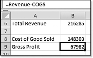
- Move the cell pointer back to the formula cell and look in the formula bar. You can see that Excel has built the formula
=Revenues-COGS, as shown in Figure 18.6. In theory, this formula is self-documenting and easier to understand than=C6-C8.
Figure 18.6. New formulas created after names have been assigned reflect the cell names in the formula.
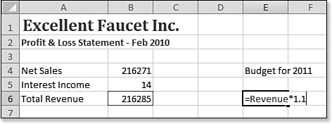
You can also type a formula that uses names directly in a cell. For example, Figure 18.7 shows =Revenue*1.1 entered in Cell E6. When you press Enter, Excel recognizes this formula and multiplies Cell A6 by 1.1.
Figure 18.7. You can type formulas to reference existing cell names.
However, a problem crops up when one of the cells in the formula contains a name—especially if that name is defined strictly for navigational purposes. In this case, Excel creates an absolute reference to that cell. When you copy a formula that contains a name, the copied formula always points to the name. This can lead to unhappy results.
Here is an example to show how easily this can happen.
Figure 18.8 shows Cell A2 named SectionThree so that the name can be used as a bookmark.
Figure 18.8. Cell A2 is named Section Three to aid navigation.
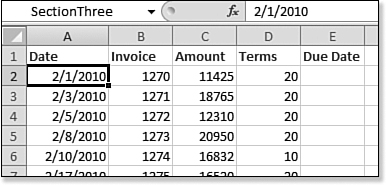
In Cell E2 you enter a formula to calculate a due date. Using the mouse method, you type =, touch Cell A2 with the mouse, type +, and then touch Cell D2 with the mouse. Instead of entering the formula =A2+D2, you end up with the formula =SectionThree+D2.
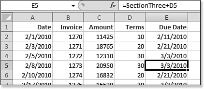
Select Cell E2 and double-click the fill handle to copy the formula down to all rows. Examine the formula in Cell E5. As shown in Figure 18.9, although Cell D2 was correctly changed to Cell D5 in the copied formula, this cell and all the remaining cells in Column E are incorrectly pointing to Cell A2 because it was previously defined as a named range.
Figure 18.9. When you copy this formula, every cell points at Cell A2 because that cell previously had a defined name.
To overcome this problem, use care when entering the original formula: Type =, type A2+, and then touch Cell D2. This overrides Excel’s default behavior of automatically converting relative reference names to preexisting range names.
Retroactively Applying Names to Formulas
When you learn the trick that was discussed in the “Using Named Ranges to Simplify Formulas” section, you might start naming all the input cells in your workbook, hoping that all the preexisting formulas will take on the new names. Unfortunately, this does not work automatically.
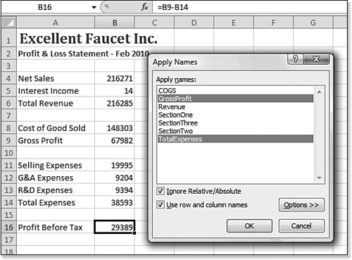
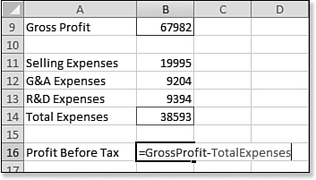
In Figure 18.10, the formula in Cell B16 was entered first. Later, Cells B9 and B14 were given the names GrossProfit and TotalExpenses, respectively. However, the preexisting formula in B16 continues to reflect the cell addresses instead of the names.
Figure 18.10. The legacy formula in Cell B16 does not reflect the new named ranges. Use Name a Range, Apply to display this dialog.
To make the names become part of existing formulas, you have to use the Apply command. To do this, follow these steps:
- On the Formulas tab, select the drop-down next to Define Name and select Apply Names. The Apply Names dialog appears, as shown in Figure 18.10.
- Choose as many names as you want in the Apply Names box. In this example, you should choose at least GrossProfit and TotalExpenses and then click OK. Any existing formulas that point to these named cells change to include the cell names in the formula, as shown in Figure 18.11.
Figure 18.11. After you apply names, existing formulas are rewritten.
![]() To watch a video of retroactively applying names to formulas, search for “Excel In Depth 18” at YouTube.
To watch a video of retroactively applying names to formulas, search for “Excel In Depth 18” at YouTube.
Tip
![]()
If you recently defined the names, those names will be preselected when you open the Apply Names dialog.
Using Names to Refer to Multiple-Cell Ranges
It is possible to define a name that refers to a larger range of cells. For example, you can select C11:C13 in Figure 18.12 and type a name such as Expenses into the Name box.
Figure 18.12. A name can refer to a rectangular range.
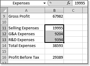
If you later select Expenses from the Name box, your cursor moves to Cell C11, and the entire range is selected. Having a name apply to a range allows formulas such as =Sum(Expenses).
Dealing with Invalid Legacy Naming
To prevent confusion, a valid cell address may not be used as a name. In legacy versions of Excel, this eliminated names from A1 through IV65536.
Excel 2010 has columns named A through Z, AA through ZZ, and AAA through XFD. The same rule applied to Excel 2010 now invalidates names that start with IW through ZZ and AAA through XFD.
You can think of many three-letter names such as Tax2007 and ROI5 that might have been common in Excel 2003. Although those are perfectly legal in Excel 2003, they are no longer valid in Excel 2010 because they duplicate existing cell addresses in Excel2010.
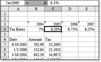
Figure 18.13 shows an Excel 2003 workbook that contains names such as Tax2004, Tax2005, and so on.
Figure 18.13. In Excel 2003, a range named Tax2004 for Cell B4 was perfectly legal because with only 256 columns, there was not a column called Tax.
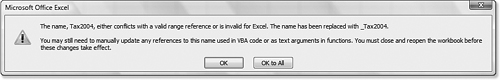
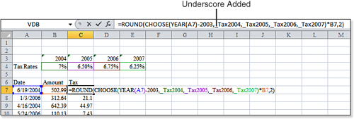
You can open this workbook in Excel 2010. The workbook initially opens in Compatibility mode, with columns only through IV. When you attempt to save the file as an Excel 2010 workbook, Excel warns you of the first named range that must be changed. In Figure 18.14, Tax2004 is being changed to _Tax2004.
Figure 18.14. When you try to save the Excel 2003 workbook as an Excel 2010 file, the established names must be changed.
Excel attempts to warn you about every existing name that must be changed. You can either click OK to each message or skip them by clicking OK to All. Note that after the Save As, the workbook is still in Compatibility mode. Close the workbook and then reopen it to see the new names.
Caution
![]()
Excel is not able to update some formulas. It would be efficient to rewrite the formula in Figure 18.13 as =B7*INDIRECT ("TAX"&YEAR(A7)). During the conversion of names from TAX2004 to _TAX2004, Excel will not update your formula to refer to "_TAX". Formulas such as these will fail after the conversion. You will have to edit the formula manually.
Excel does a great job of updating the names and the formulas that use invalid names. Figure 18.15 shows the Excel 2003 worksheet after it is converted to Excel 2010. Each name now has an underscore at the beginning.
Figure 18.15. Excel correctly updated these references.
Adding Many Names at Once from Existing Labels and Headings
With Excel 2010 you can add many names in a single command, particularly if the names exist as labels or headings adjacent to the cells.
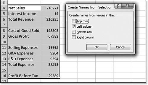
Suppose you have a worksheet with a series of labels in Column A and values in Column B. One example is shown in Figure 18.16. To do a wholesale assignment of names to the cells in Column B, follow these steps:
- Select the range of labels and the cells to which they refer. In this example, this would be A4:B16.
- Select Formulas, Names, Create from Selection. Excel displays the Create Names from Selected Range dialog.
- Because the row labels are in the left column of the selected range, select Left Column and then click OK, as shown in Figure 18.16.
Figure 18.16. When you make this selection, Excel uses the text values in the left column to assign names to all the nonblank cells in Column B of this range.
Excel does a fairly good job of assigning the names. Spaces are replaced with underscores to make the names valid. Figure 18.17 shows the names created as a result of this command. In this example, Cell B4 is assigned the name Net_Sales. Cell C8 is assigned the name Cost_of_Good_Sold. In Row 12, where the label contains an ampersand (&), Excel replaces the ampersand with an underscore, to form the name G_A_Expenses. Although this is not as meaningful as it could be if you wrote the name yourself, it is still pretty good.
Figure 18.17. Excel replaces spaces and ampersands with underscores when creating names from a selection.
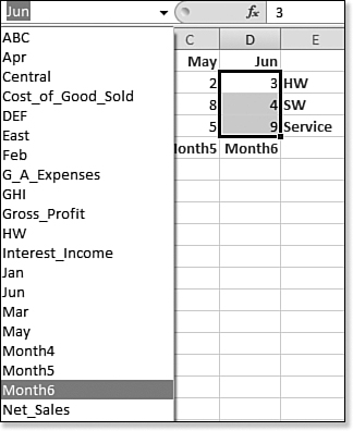
In Excel 2010, you can apply names by using both the row labels and column headings at the same time. In Figure 18.18, the selections in the Create Names from Selected Ranges dialog mean that six new names will be added to the workbook. For example, Jan will refer to B2:B4.
Figure 18.18. In Excel 2010, you can create names based on the row labels and column headers at the same time.

Caution
![]()
If Cell A12 were G & A Expenses, Excel would replace every space and ampersand with an underscore, creating the name G___A_Expenses.
The Create Names from Selected Range dialog is so flexible that it will even let you select all four options at once. If you select all the check boxes in the Create Names from Selected Range dialog and then click OK, 12 new names will be added to the workbook (see Figure 18.18).
Figure 18.19. You can create names based on labels on all four edges of a range. However, it is difficult to imagine a scenario in which you would want to do this.
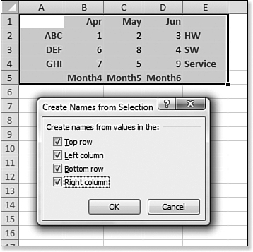
In this example, the name Jun will refer to D2:D4. The name Month6 will also refer to D2:D4. If you select Month6 from the drop-down, Excel selects D2:D4, as shown in Figure 18.20. However, the name in the Name box reflects Jun because that is the first name, alphabetically, that applies to that range.
Figure 18.20. D2:D4 is called both Jun and Month6.
Managing Names
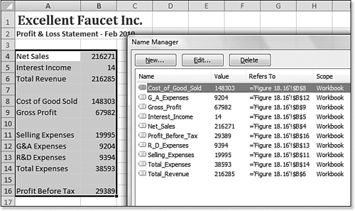
Excel 2007 was a great improvement over legacy Excel versions in terms of managing names. Whereas older versions of Excel used the Insert Names dialog to manage names, Excel 2007 offered the Name Manager dialog, shown in Figure 18.21. To open this dialog, click the Name Manager icon on the Formulas tab.
Figure 18.21. Click Name Manager to display the vastly improved Names Manager dialog.
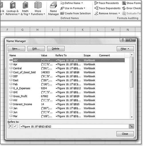
The Name Manager dialog shows the five fields for each name. Initially, certain columns may not be wide enough to show all the text in each column. You can resize the entire dialog by using the triangle in the lower-right corner. You can also resize columns by dragging the vertical bars between the column headings.
Listed below are the columns in the Name Manager dialog:
• Name—Shows the current name.
• Value—Shows the current value. If the Name column refers to a rectangular range, each value in the range is shown in the Value column.
• Refers To—Shows the formula defined for the name. This might be a reference to a cell address, a constant value, or a formula.
• Scope—Indicates whether the name applies to the whole workbook or just to a certain worksheet.
• Comment—Shows any comments you might have typed when you originally defined a name.
Working with the Name Manager dialog is straightforward:
• To create a new name, click the New Name button.
• To delete a name, highlight the name and click Delete Name. However, this should be done with caution. If the name is being used, all the formulas that point to that name change to #NAME? errors.
• To view the cells represented by a certain name, select the name from the Name column of the dialog and then click at the end of the Refers To box. Excel shows you the section of the worksheet behind the dialog.
• To reassign a name to a different set of cells, choose the name from the Name column of the dialog and then click in the Refers To box. On the worksheet, point to the new location for the name. After you select a new location, click the check box to accept the new location. Click the x button to revert to the original location.
• If you click a name from the Name column of the dialog and then click Edit Name, you have an opportunity to add or change the comment to the name or to change the scope.
• When you modify an existing name in the Name column of the dialog, any formulas that specifically reference that name are updated to point to the new cell.
Filtering the Name Manager Dialog
In the upper-right corner of the Name Manager dialog is a button labeled Filter that can be clicked to access many powerful options. If you have defined names that have scope only to a worksheet, you can select Names Scoped to Worksheet to limit the Name Manager dialog to only those names, as shown in Figure 18.22.
Figure 18.22. The Filter button allows you to narrow the scope to certain names.
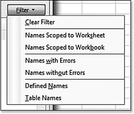
Following are the options in the Filter drop-down:
• Clear Filter—Restores the list to the complete list.
• Names Scoped to Worksheet—Shows all worksheet-level names for the active worksheet and other worksheets.
• Names Scoped to Workbook—Shows all the global names that are scoped to a workbook.
• Names with Errors—Finds all names where the value is a cell error. Often, stray names left behind after copying a worksheet to a new workbook have #REF! errors. You can use the Names with Errors filter to find those names.
• Names Without Errors—Hides any invalid names.
• Defined Names—Specifies the names defined using the techniques described in this chapter. This option removes names defined as a result of creating pivot tables or formatting ranges as tables.
• Table Names—Shows only the values of table names. When you define a range as a table, the entire table is given a name such as Table1.
Using a Name to Simplify an Absolute Reference
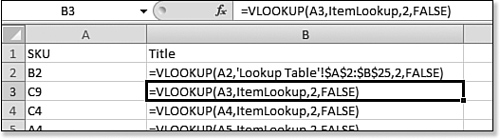
A common scenario is when a formula such as VLOOKUP is used in a data set to look up data on another worksheet. You might enter a VLOOKUP formula in Cell B2 and copy it to hundreds of records. The formula in Cell B2 might be =VLOOKUP(A2,'Lookup Table'!A2:B25,2,False). As you copy this formula to Row 3, the reference in the second argument will incorrectly change to 'Lookup Table'!A3:B26. When you need the reference to always point to A2:B25, you can add dollar signs to the reference: $A$2:$B$25.
If you will be frequently adding VLOOKUP formulas that will point to 'Lookup Table'!$A$2:$B$25, it can get tedious to continually use the syntax. After all, it is a confusing mix of dollar signs, apostrophes, and exclamation points.
To simplify the VLOOKUP formula, give A2:B25 a name such as ItemLookup. Then, the formula simply becomes =VLOOKUP(A2,ItemLookup,2,False). As you copy the formula down, it continues to point to A2:B25 on the Lookup Table worksheet. Figure 18.23 compares the formula without a name in B2 and the formula with a name in B3.
Figure 18.23. The formula in B3 is easier to type because it uses a named range for the lookup table.
Using a Name to Hold a Value
So far, all the names defined in this chapter have referred to a cell or a range of cells. It is possible to assign a constant value to a name by using the New Name dialog. You might do this to hold a value that could possibly change, but would likely rarely change, such as a sales tax rate.
To use a name to hold a value, follow these steps:
- Either click the Name a Range icon or the Name Manager icon and then click Add Names. Both icons are located in the Defined Names group on the Formulas tab. The New Name dialog appears.
- In the Name field of the New Name dialog, type a name such as Sales_Tax.
- In the Refers To box, remove any existing cell reference and type the new value (=6.5%, as shown in Figure 18.24).
Figure 18.24. In the New Name dialog, you can assign a constant value to a name.

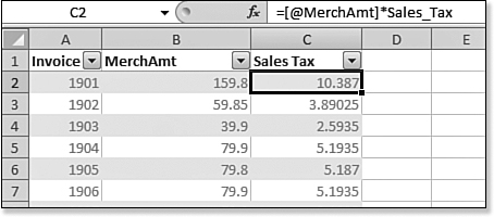
- Write formulas that refer to the new name such as
Sales_Tax. The formula might be something like=C2*Sales_Tax. In Figure 18.25, the range has been defined as a table. Thus, the formula of=[@MerchAmt]*Sales_Taxuses both a table name in square brackets and the defined nameSales_Tax.Figure 18.25. MerchAmt, in square brackets, is a field name in the table. Sales_Tax is a defined name.
Caution
![]()
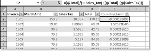
Use care when viewing potentially ambiguous references such as Sales_Tax and [@ Sales Tax] as shown in Figure 18.26. Remember, the name in square brackets is a table name assigned automatically by Excel.
Figure 18.26. With defined names and table column names floating around, ambiguous formulas like this can turn up.
The advantage of using a name to refer to a constant is that if your tax rate changes, you can edit the value defined in the name, and all the formulas in the workbook will recalculate. To edit an existing name, click the Name Manager, click the name, and then select Edit Name.
Assigning a Formula to a Name
Although names are traditionally used to refer to cells or constant values, an interesting use is to use a name to refer to a formula.
Notice the Refers To box in Figure 18.27. Although the value in this figure is a standard name that refers to a single cell, the Refers To box contains = at the beginning, which means this named range is actually a formula.
Figure 18.27. Even a simple named range can be a formula assigned to a name.

As described in the following sections, assigning a formula to a name can be useful in a variety of situations.
Using Basic Named Formulas
A named formula allows you to replace a complicated formula with an easy to remember name. In this basic case, the formula does not contain cell references.
For example, suppose you have discovered a fairly complex formula that would be difficult to remember, such as the formula shown in Figure 18.28.
Figure 18.28. You can assign a complicated formula to a simpler name.
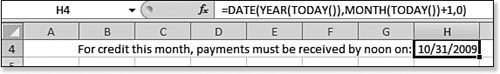
In this case, you could assign the formula =Date(Year(Today()),Month(Today())+1,0) to a name such as MonthEnd, as shown in Figure 18.29
Figure 18.29. After a formula has been assigned to a name, you can use it as you would a constant.

You could then use =MonthEnd in any cell to calculate the end of the current month.
Using Dynamic Named Formulas
An interesting example of a named formula is a reference that dynamically expands as more data is filled down a column.
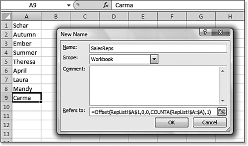
Suppose that you have a list of valid sales reps on a hidden RepList to be used as the list for a data validation drop-down. The list might extend from A1:A9 today, but as new sales reps are hired, the list may expand to A10, A11, A12, and so on.
The OFFSET() function has a parameter that specifies that a range should extend for X rows. If you use COUNTA to return the number of rows, you can create a formula to dynamically expand or contract as cells are filled in or deleted. In theory, you would set up a formula to point to this range: =OFFSET(RepList!A1,0,0,COUNTA(RepList!A:A),0). However, absolute references should be used in the definition. In Figure 18.30, for example, the formula assigned to RepList is =OFFSET(Rep List!$A$1,0,0,COUNTA(RepList!$A:$A),1).
Figure 18.30. This formula can expand to include the number of entries in Column A.
The name automatically expands as new entries are added. To make use of this name in an in-cell drop-down, follow these steps:
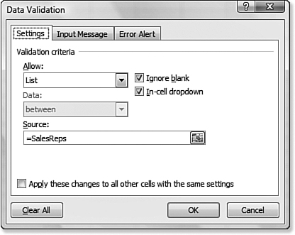
- Select Data, Data Validation.
- Change the Allow drop-down to List.
- In the source box, type =SalesReps.
- Leave the In-cell drop-down box selected.
The completed dialog box is shown in Figure 18.31.
Figure 18.31. You can set up data validation to use a dynamic name.
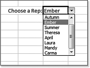
Initially, the cell with validation offers a drop-down that lists the nine current reps, as shown in Figure 18.32.
Figure 18.32. The result of adding data validation to a cell.
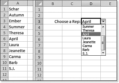
When the list on RepList is edited, the drop-down is automatically updated. For example, in Figure 18.33, you can see that Jeanette replaced Mandy, and two new reps were added. The window on the left shows the new list on RepList, and the window on the right shows the current drop-down list.
Figure 18.33. As the list on RepList changes, the dynamic formula expands to include the new cells in the list.
You can use a similar technique to make a chart series expand as new months are added.
![]() For details on charting, see Chapter 32, “Using Excel Charts.”
For details on charting, see Chapter 32, “Using Excel Charts.”
Using a Named Formula to Point to the Cell Above
In the example shown in Figure 18.33, it was important to make sure that all references were absolute. Although it seems strange, it is possible to make use of a relative reference in a named formula. However, this should be done only if you understand one slightly buggy gotcha and two cautions if you use VBA or share the workbook with someone using Excel 97.
• The gotcha happens in workbooks with multiple worksheets. A relative formula will work fine on the original worksheet, but incorrectly when used on another worksheet. A workaround that starts the reference with an ! solves this problem.
• The first caution is that this method fails if you are using VBA macros and the macro causes the worksheet to calculate.
• The second caution is that this method will crash Excel if the workbook is opened in Excel 97.
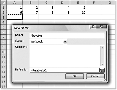
In Figure 18.34, the cell pointer is on the Relative worksheet in Cell A3. The name AboveMe is being defined as pointing to Cell A2. However, in the Refers To box, press F4 three times to remove all the dollar signs from the reference.
Figure 18.34. Defining a relative reference in a named formula.
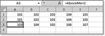
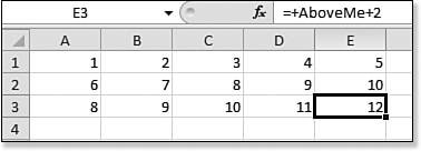
This relative formula initially appears to work perfectly. Cells A3:E3 in Figure 18.35 all contain the formula =AboveMe+2.
Figure 18.35. In this example, the relative reference in the named formula is working fine.
However, if you go to Sheet2 and enter the formula =AboveMe+2 in Cells A3:E3, the formula returns the value from Row 2, but from the Relative sheet instead of the current worksheet. Figure 18.36 shows the answer 8 when you would expect 103.
Figure 18.36. The relative reference in the named formula fails on another sheet.
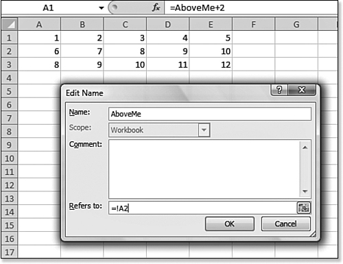
The solution is to edit the name. To do so, remove the reference to Sheet1, leaving a definition of =!A2, as shown in Figure 18.37.
Figure 18.37. Edit the formula to point to =!A2.
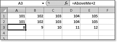
Now, when you close the Name Manager dialog, the formulas work as expected, as shown in Figure 18.38.
Figure 18.38. The relative reference of =!A2 now works as expected.