
12. Using Powerful Functions: Logical, Lookup, and Database Functions
This chapter covers four groups of workhorse functions. If you process spreadsheets of medium complexity, you will turn to logical and lookup functions regularly.
• The logical functions, including the ubiquitous IF function, help make decisions.
• The information functions might be less important than they once were, now that Microsoft has added the IFERROR function, but INFO, CELL, and TYPE still come in handy.
• The lookup functions include the powerful VLOOKUP, MATCH, and INDIRECT functions. These functions are invaluable, particularly when you are doing something in Excel when it would be better to use Access. In addition, let’s face it; with 1.1 million rows in Excel 2010, we will all do more things in Excel that should be done in Access.
• Finally, the database functions provide the DSUM functions. Even though these functions fell out of favor with the introduction of pivot tables, they are a powerful set of functions that are worthwhile to master.
Table 12.1 provides an alphabetical list of all Excel 2010’s logical functions. Detailed examples of these functions are provided later in this chapter.
Table 12.1. Alphabetical List of Logical Functions

Table 12.2 provides an alphabetical list of all Excel 2010’s information functions. Detailed examples of these functions are provided in the remainder of the chapter.
Table 12.2. Alphabetical List of Information Functions

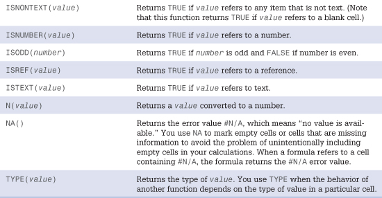
Table 12.3 provides an alphabetical list of all Excel 2010’s lookup functions. Detailed examples of these functions are provided later in this chapter.
Table 12.3. Alphabetical List of Lookup Functions

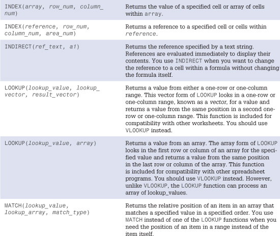
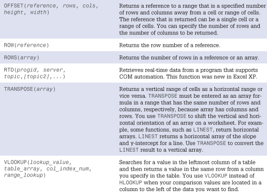
Table 12.4 provides an alphabetical list of all of Excel 2010’s database functions. Detailed examples of these functions are provided later in this chapter.
Table 12.4. Alphabetical List of Database Functions
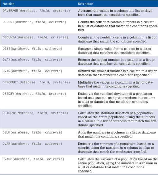
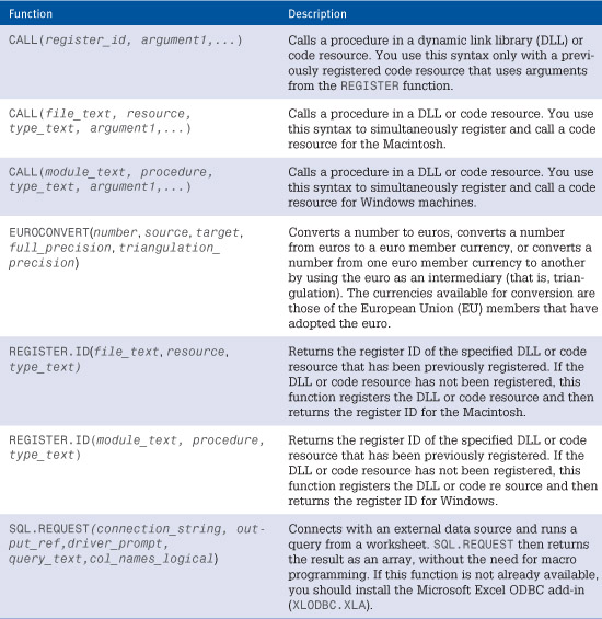
Table 12.5 provides an alphabetical list of all of Excel 2010’s external functions. Detailed examples of these functions are provided later in this chapter.
Table 12.5. Alphabetical List of External Functions
Examples of Logical Functions
With only seven functions, the logical function group is one of the smallest in Excel. The IF function is easy to understand, and enables you to solve a variety of problems.
Using the IF Function to Make a Decision
Many calculations in our lives are not straightforward. Suppose that a manager offers a bonus program if her team meets its goals. Or perhaps a commission plan offers a bonus if a certain profit goal is met. These types of calculations can be solved by using the IF function.
Syntax: IF(logical_test,value_if_true,value_if_false)
There are three arguments in the IF function. The first argument is any logical test that results in a TRUE or FALSE. For example, you might have logical tests such as these:
A2>100
B5="West"
C99<=D99
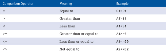
All logical tests involve one of the comparison operators shown in Table 12.6.
Table 12.6. Comparison Operators
The remaining two arguments are the formula or value to use if the logical test is true and the formula or value to use if the logical test is false.
When you read an IF function, you should think of the first comma as the word then and the second comma as the word otherwise. For example, =IF(A2>10,25,0) would be read as “If A2>10, then 25; otherwise, 0.”
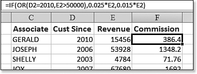
Figure 12.1 calculates a sales commission. The commission rate is 1.5 percent of revenue. However, if the gross profit percentage is 50 percent or higher, the commission rate is 2.5 percent of revenue.
Figure 12.1. In Rows 2, 4, and 5 the commission is 1.5 percent. In Rows 3 and 6 the commission is 2.5 percent.

In this case, the logical test is H2>=50 percent. The formula if that test is true is 0.025*F2. Otherwise, the formula is 0.015*F2. You could build the formula as =IF(H2>=50%,0.025*F2,0.01 5*F2).
Note
![]()
Mathematicians would correctly note that in both the second and third arguments of the formula =IF(H2>=50%,0.025*F2,0.015*F2), you are multiplying by F2. Therefore, you could simplify the formula by using =IF(H 2>=50%,0.025,0.015)*F2.
Using the AND Function to Check for Two or More Conditions
The previous example had one simple condition: If the value in Column H was greater than or equal to 50 percent, the commission rate changed.
However, in many cases you might need to test for two or more conditions. For example, suppose that a retail store manager offers a $25 bonus for every leather jacket sold on Fridays this month. In this case, the logical test requires you to determine whether both conditions are true. You can do this with the AND function.
Syntax
AND(logical1,logical2,...)
The arguments logical1,logical2,... are from 1 to 255 expressions that evaluate to either TRUE or FALSE. The function returns TRUE only if all arguments are TRUE.
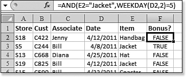
In Figure 12.2, the function in Cell F2 checks whether Cell E2 is a jacket and whether the date in Cell D2 falls on a Friday:
=AND(E2="Jacket",WEEKDAY(D2,2)=5)
Figure 12.2. The AND function is TRUE only when every condition is met.
Using the AND Function to Compare Two Lists
The AND function can handle up to 255 expressions. Each expression can contain a range that might contain many instances of TRUE or FALSE.
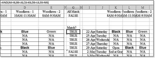
A common issue is figuring out whether two worksheets are identical. In Figure 12.3, Columns A:E contain the original worksheet. After this worksheet was passed among several co-workers, it ended back at your desk. Follow these steps to compare the two worksheets:
- Leave three blank columns—Columns F, G, and H—to the right of your original data.
- Copy the data range of the returned worksheet. Paste this copy, starting in Column I of the original worksheet.
- Add the heading All Match? in Column G.
- Add a formula in Column G to compare whether each of the cells in the original data set matches the cells in the returned data set. Add the formula =
AND(A6=I6,B6=J6,C6=K6,D6=L6,E6=M6)in Cell G6 to compare all five cells in the data set. - Copy the formula down Column G from Cell G6 to match the number of rows in the data set.
- In Cell G2, enter an
ANDformula to test whether all the formulas in Column G areTRUE. Even though this range contains more than 255 cells, it is still valid to use it as one of the expressions in theANDfunction. The formula in G2 is=AND(G6:G999). This is a quick way to find out whether every row is identical without having to scroll through pages of data, looking for a singleFALSEresult. If Cell G2 returnsTRUE, you know that the original and returned worksheets are identical. If Cell G2 returnsFALSE, you know that one or more of the rows were changed. - Select G6:G999. From the Home tab, select Find & Select, Find. The Find and Replace dialog appears.
- In the Find and Replace dialog, type
FALSEinto the Find What box. You must click the Options button and change the Look In drop-down from Formulas to Values to find formulas that result in a value ofFALSE.
Figure 12.3. AND can test whether a large range of logical tests are all TRUE.
Tip
![]()
Instead of using the AND function, you can multiply the conditions. =(A6=I6)*(B6=J6)*(C6=K6)*(D6*L6)*(E6=M6) will return 1 if all the conditions are true and zero if any one of the conditions is false. Alternatively, you can type =AND(A6:E6=I6:M6) and press Ctrl+Shift+Enter to have AND evaluate the array of comparisons.
Using OR to Check Whether Any Conditions Are Met
You might have a situation in which a certain formula is based on meeting one of several conditions. A sales manager may want to reward big orders and orders from new customers. The manager may offer a commission bonus if the order is over $50,000 or if the customer is a new customer this year.
To test whether a particular sale meets either condition, use the OR function. The OR function returns TRUE if any condition is TRUE and returns FALSE if none of the conditions are TRUE.
Syntax
OR(logical1,logical2,...)
The OR function checks whether any of the arguments are TRUE. It returns a FALSE only if all the arguments are FALSE. If any argument is TRUE, the function returns TRUE.
The arguments logical1,logical2,... are 1 to 255 conditions that can evaluate to TRUE or FALSE.
In Figure 12.4, the logical test to see if revenue is over $50,000 is E2>50000. The logical test to see if the customer is new this year is D2=2010. The structure of this OR function is =OR(D2=2010,E2>50000).
Figure 12.4. OR checks whether a record meets at least one of several criteria.
You can use the OR function as the first argument to the IF function to produce the formula shown in Cell F2: =IF(OR(D2=2010,E2>50000),0.025*E2,0.015*E2).
Nesting IF Functions
The IF function offers only two possible formulas. Either the logical test is TRUE and the first formula is used, or the logical test is FALSE and the second formula is used.
Many situations have a series of choices. For example, in a human resources department, annual merit raises may be given based on the employee’s numeric rating in an annual review, in which employees are ranked on a 5-point scale. The rules for setting the raise are as follows:
• 4.5 or higher: 5 percent raise
• 4 or higher: 4.5 percent raise
• 3.25 or higher: 3 percent raise
• 2.5 or higher: 1 percent raise
• Under 2.5: no raise
You can build the IF statement by following these steps:
- Test for the highest condition first. Excel stops testing when the first condition is met. If the first test checks to see if an employee had a rating of higher than 2.5, then anyone from 2.5 to 5 receives a 1 percent raise. In this case, you want to give a 5 percent raise to anyone with a rating of 4.5 or greater. Therefore, the formula starts out as =
IF(B2>=4.5,5%,.Caution

These
IFformulas are hard to read. There is a temptation to use them for situations with very long lists of conditions. Whereas Excel 2003 prevented you from nesting more than seven levels ofIFfunctions, Excel 2007 and later allows you to nest up to 64 IF statements. Before you start nesting that many IF statements, you should consider usingVLOOKUP, which is explained later in this chapter. - There is only one argument left in the current IF function—the argument for
value_if_false. Instead of using a value as the third argument, start a second IF function to be used if the first test isFALSE. This IF function starts outIF(B2>=4,4.5%,. Combine this start of an IF function with the firstIFfunction:=IF(B2>=4.5, 5%,IF(B2>=4,4.5%,. - There are still three possible raise levels and only one argument left in the second IF function. Start a third IF function to be used as the
value_if_falseargument for the second IF function:IF(B2>=3.25,3%,. At this point, if the employee did not rank above 3.25, only two possibilities are left. The employee is either 2.5 and above for a 1 percent raise, or he or she gets no raise. - Create the fourth
IFfunction:IF(B2>=2.5,1%,0). - With the four
IFfunctions, be careful to provide four closing parentheses at the end of the function: =IF(B2>=4.5,5%,IF(B2>=4,4.5%,IF(B2>=3.25,3%,IF(B2>=2.5,1%,0%))))(see Figure 12.5).Figure 12.5. This formula contains four nested
IFfunctions.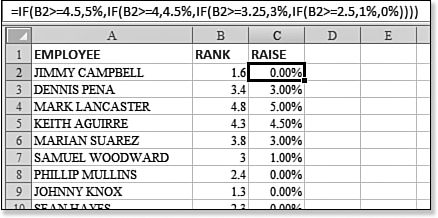
Using the TRUE and FALSE Functions
There are two remaining functions in the logical group, but you should not need to use either of them. If you encounter a function with either the TRUE or FALSE function, you can replace the function with the value TRUE or FALSE. Microsoft added TRUE and FALSE to provide compatibility with other vendors’ spreadsheet programs.
A formula such as =IF(OR(A2>5,B2=0),TRUE(),FALSE()) can be rewritten as =IF(OR(A2>5,B2=0),TRUE,FALSE). If you are trying to return TRUE or FALSE, you can simply use the Boolean expression: =OR(A2>5,B2=0).
Using the NOT Function to Simplify the Use of AND and OR
In the language of Boolean logic, there are typically NAND, NOR, and XOR functions, which stand for Not And, Not Or, and Exclusive Or. To simplify matters, Excel offers the NOT function.
Syntax
NOT(logical)
Quite simply, NOT reverses a logical value. TRUE becomes FALSE, and FALSE becomes TRUE when processed through a NOT function.
For example, suppose you need to find all flights landing outside of Oklahoma. You can build a massive OR statement to find every airport code in the United States. Alternatively, you can build an OR function to find Tulsa and Oklahoma City and then use a NOT function to reverse the result: =NOT(OR(A2="Tulsa",A2="Oklahoma City")).
Using the IFERROR Function to Simplify Error Checking
The IFERROR function, which was introduced in Excel 2007, was added at the request of many customers. To help understand the IFERROR function, you need to understand how error checking was performed during the 22 years before Excel 2007 was released.
Figure 12.6 shows a typical spreadsheet that calculates a ratio of sales to hours. Even though this formula works most of the time, in occasional records, the divisor is zero, and the formula returns a #DIV/0 error.
Figure 12.6. The zero in the divisor in Row 5 causes a division-by-zero error.
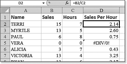
The typical way to deal with this in legacy versions of Excel was to set up an IF function to check whether the divisor was zero: =IF(C5=0,0,B5/C5). If the divisor were zero, the formula returns a zero as the result. Otherwise, the formula performs the calculation.
In legacy versions of Excel, it was typical to use this type of IF formula on thousands of rows of data. The formula is more complex and takes longer to calculate than the new IFERROR function. However, this particular formula is tame compared to some of the formulas needed to check for errors.
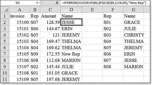
A common error occurs when you use the VLOOKUP function to retrieve a value from a lookup table. In Figure 12.7, the VLOOKUP function in Cell D2 asks Excel to look for the rep number S07 from Cell B2 and find the corresponding name in the lookup table of F2:G9. This works great, returning JESSE from the table. However, a problem arises when the sales rep is not found in the table. In Row 7, rep S09 is new and has not yet been added to the table, so Excel returns the #N/A result.
Figure 12.7. An #N/A error means that the value is not in the lookup table.
If you wanted to avoid #N/A errors, the generally accepted workaround in legacy versions of Excel was to write this horrible formula:
=IF(ISNA(VLOOKUP(B7,$F$2:$G$9,2,FALSE)),"New Rep", VLOOKUP(B7,$F$2:$G$9,2,FALSE))
In English, this formula says to first find the rep name in the lookup table. If the rep is not found and returns the #N/A error, then use some other text, which in this case are the words New Rep. If the rep is found, then perform the lookup again and use that result.
Because VLOOKUP was one of the most time-intensive functions, it was horrible to have Excel perform every VLOOKUP twice in this formula. In a data set with 50,000 records, it could take minutes for the VLOOKUP to complete. Microsoft wisely added the new IFERROR function to handle all these error-checking situations.
Syntax
IFERROR(value,value_if_error)
The advantage of the IFERROR function is that the calculation is evaluated only once. If the calculation results in any type of an error value such as #N/A, #VALUE!, #REF!, #DIV/0!, #NUM!, #NAME?, or #NULL!, Excel returns the alternate value. If the calculation results in any other valid value, whether it is numeric, logical, or text, Excel returns the calculated value.
The formula from the preceding section can be rewritten as =IFERROR(VLOOKUP(B7, $F$2:$G$9,2,FALSE),"New Rep") (see Figure 12.7). This calculation is easier to write and calculates much more quickly than the method required in legacy versions of Excel.
Caution
![]()
If you will be sharing your workbook with people who use legacy versions of Excel, you should avoid using IFERROR. Instead, you should test for the various error conditions as described in the next section.
Examples of Information Functions
Found under the More Function icon, the 17 information functions return eclectic information about any cell. Ten of the 17 functions are called the IS functions because they test for various conditions.
Using the IS Functions to Test for Errors
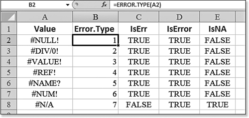
Figure 12.8 shows the results of the following four functions for testing error values:
• ISERROR—This function evaluates whether a calculation or value results in any type of error. If people using only Excel 2007 or later will use your workbooks, you should use the IFERROR function instead of ISERROR. However, if you need to share your workbook with people using legacy versions of Excel, you should use ISERROR, which is usually combined with an IF function. Here is an example: =IF(ISERROR(A2),"Unknown",A2).
• ISERR—This function is similar to ISERROR, except it does not report #N/A errors.
• ISNA—This function specifically tests whether a result returns an #N/A error.
• ERROR.TYPE—This function lets you know specifically what error is being returned. This function returns a value from 1 through 7 to indicate #NULL!, #DIV/0!, #VALUE!, #REF!, #NAME?, #NUM!, and #N/A, respectively. It is possible to write a lengthy formula such as the following to decode these values and provide a friendlier error message:
=IF(NOT(ISERROR(A2)),A2,CHOOSE(ERROR.TYPE(A2),"Null Value Found",
"Division by Zero","Invalid Value","Missing Reference","Undefined Name",
"Numeric Error","Value Not Available"))
Figure 12.8. The results of IS functions for detecting errors.
Note
![]()
Mathematicians in the audience may suggest that you could just as easily use =MOD(A2,2)=0 to figure out whether a number is even. However, unless you are a mathematician, it is far easier to remember =ISEVEN().
Using IS Functions to Test for Types of Values
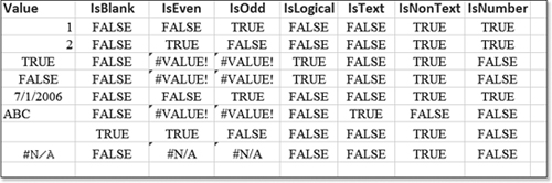
Figure 12.9 shows the results for the seven remaining IS functions. Each of these functions reveals if a value contains a particular type of value:
• ISBLANK—This function returns TRUE only if a cell is completely empty. A cell that contains several spaces is not considered blank. Even a cell that contains a single apostrophe and no spaces is not considered blank by the ISBLANK function. It would have been more appropriate if the folks at Lotus 1-2-3 would have called this the @IsEmpty function, but you are stuck with the bad name now that it has been in use forever.
• ISEVEN—This function indicates if a number is evenly divisible by 2. Note that Cell C8 is an empty cell, which is considered zero and reports as even. Using a date as the value in ISEVEN returns a value, but that value does not make sense. Using text or logical values in the ISEVEN function causes a #VALUE! error.
• ISODD—This function indicates whether a number is not evenly divisible by 2. An empty cell is considered zero and returns FALSE to ISODD. The same limitations listed for ISEVEN apply to ISODD. In addition, if your value contains decimal places, they are ignored by both the ISEVEN and ISODD functions. Numbers such as 1.02, 1.2, 1.5, 1.9, 1.99999999 all return TRUE for the ISODD function.
• ISLOGICAL—This function indicates if the value is either TRUE, FALSE, or an expression that results in TRUE or FALSE.
• ISTEXT—This function returns TRUE if the value contains text. This is good for finding values such as ABC in Cell A16 and for finding cells that look like numbers but are actually stored as text.
• ISNONTEXT—This returns TRUE for anything that is nontext. Numbers, logicals, dates, empty cells, and even error cells return TRUE for ISNONTEXT.
• ISNUMBER—This function returns TRUE for numeric cells and dates. Note that although the empty Cell A8 can be calculated as even in Cell C8, it returns FALSE to ISNUMBER in Cell H8.
Figure 12.9. The results of IS functions for detecting certain types of values.
Note
![]()
Note a very important distinction here: ISLOGICAL does not tell you whether a value is FALSE. It merely indicates that the expression results in one of the valid logical values of TRUE or FALSE.
The functions in this section are nearly always used in conjunction with an IF function. For example, ZIP codes in the United States should always be five digits. This causes problems when someone keys in a ZIP code for certain eastern cities that start with a zero. For example, in Cell C6 of Figure 12.10, the proper way to key a ZIP code for Portland, Maine, is to type an apostrophe and then 04123. Most people forget the apostrophe, and Excel drops the leading zero, as shown in Cell C5.
Figure 12.10. The formula in Column D detects nontext ZIP codes and converts to text with five digits.
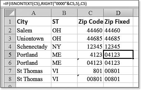
The formula in Column D, =IF(ISNONTEXT(C5),RIGHT("0000"&C5,5),C5), fixes errant ZIP codes in Column C. If the value in Column C is nontext, the program pads the left side of the ZIP code with zeros and then takes the five right-most digits.
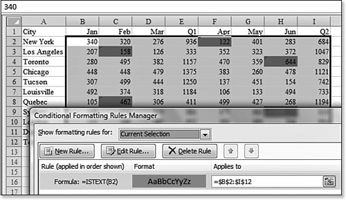
Another use of the IS functions is in the formulas for a conditional formatting rule. In Figure 12.11, a few cells were entered erroneously as text instead of numbers. Setting up a rule to mark any cells where the formula =ISTEXT(B2) is true reveals the cells that need to be updated.
Figure 12.11. An ISTEXT function is used in conditional formatting to mark any numbers erroneously entered as text.
![]() For more information on using formulas as rules for conditional formatting, see Chapter 9, “Controlling Formulas.”
For more information on using formulas as rules for conditional formatting, see Chapter 9, “Controlling Formulas.”
Using the ISREF Function
The ISREF function tests whether a value is a reference.
Syntax
ISREF (value)
ISREF returns TRUE if the value is a valid reference. Initially, this function may seem to be useless. After all, inherently you know that A2 is a valid reference, so you would not have to use a function to test it.
The following formulas return TRUE: =ISREF(A2), =ISREF(XFD1048576), and =ISREF(A2:Z99). The following formulas return FALSE: =ISREF("A2"), =ISREF(99), and =ISREF(2+2).
ISREF is useful in one special circumstance. For example, suppose you have designed a spreadsheet with the named range “ExpenseTotal”. If you are worried that someone might have deleted this particular row, you can check whether ExpenseTotal is still a valid name by using =ISREF(ExpenseTotal). Here’s an example:
=IF(ISREF(ExpenseTotal),ExpenseTotal*2,"Named Range Has Been Deleted")
Using the ISREF Function to Check a Reference
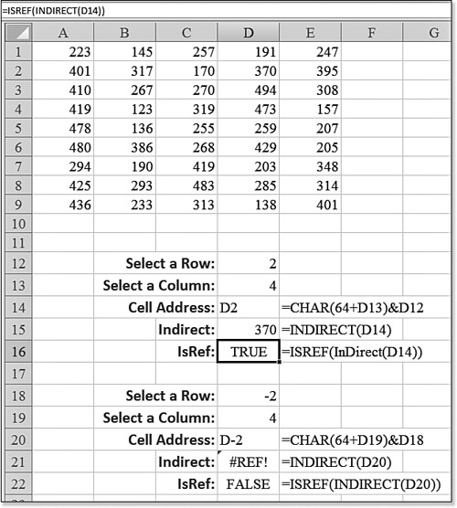
The lookup function INDIRECT allows you to build a cell reference by using a formula. In Figure 12.12, the cell address in Cell D14 is built using a formula to concatenate a column letter with a row number. Cell D15 then uses the INDIRECT function to return the value stored in the cell referenced by the formula in Cell D14. As you can imagine, this process is subject to error. Someone might enter a negative number, as shown in Cell D18. Before using the INDIRECT function, you can check if the reference in Cell D14 is a valid reference by using =ISREF(INDIRECT (D14)).
Figure 12.12. Prevent problems with Indirect by checking ISREF(INDIRECT()) first.
Using the N Function to Add a Comment to a Formula
You can call Excel’s N function a creative use for an obsolete function. Lotus 1-2-3 used to offer an N() function that converted a value as follows:
• N(any number) returned that number.
• N(a date) returned the serial number of the date.
• N(True) returned 1.
• N(False) returned 0.
• N(any error) returned the error.
• N(any text) returned 0.
None of these functions is terribly interesting. You can replicate just about any of them by referring to the value and changing the cell format.
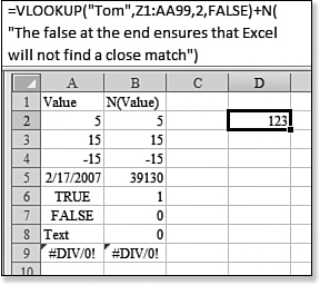
An interesting unintended use of the function is that N(any text) always returns zero. A useful trick is to insert a comment about a long formula by adding the N function to the end of the formula. However, make sure that your comment contains text. Since N(text) is zero, the outcome of the function does not change. When you come back to the formula several months later, you can see the comment in the formula bar (see Figure 12.13).
Figure 12.13. Because N of text is zero, you can store a comment in the N function.
Using the NA Function to Force Charts to Not Plot Missing Data
Suppose that you are in charge of a school’s annual fund drive. Each day, you mark the fundraising total on a worksheet by following these steps:
- In Column A, you enter the results of each day’s collection through 9 days of the fund drive (see Figure 12.14).
Figure 12.14. Using
NAin the chart on the right allows the trendline to ignore future missing data points and project a reasonable ending result.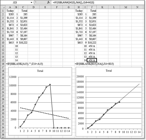
- Enter a formula in Column C to keep track of the total collected throughout the fund drive.
- To avoid making it look like the fund drive collected nothing in Days 10 through 14, enter a formula in Column C to checks whether Column A is blank. If it is, the
IFfunction inserts a null cell in Column C. For example, the formula in Cell C15 is=IF(ISBLANK(A15),"",A15+C14). - Build a line chart based on B1:C15. Add a trendline to the chart to predict future fundraising totals.
- As shown in Columns A:C of Figure 12.14, this technique fails. Even though the totals for Days 10 through 14 are blank, Excel charts those days as zero. The linear trendline predicts that your fundraising will go down, with a projected total of just over $2,000.
- Try the same chart again, but this time use the
NAfunction instead of “” in theIFstatement in step 3. The formula is shown in Cell H16, and the results are in Cell J15. Excel understands thatNAvalues should not be plotted. The trendline is calculated based on only the data points available and projects a total just under $18,000.
In many cases, you are trying to avoid #N/A! errors. However, in the case of charting a calculated column, you might want to have #N/A! to produce the correct look to the chart.
Using the INFO Function to Print Information About a Computer
The remaining information functions tell you some piece of information about a particular cell or about the computer. The INFO function is left over from Lotus 1-2-3. Some of the information it provides was useful only in Lotus. However, a few of the options may be useful to display in an Excel spreadsheet.
Syntax
=INFO(type_text)
The INFO function returns information about the current operating environment.
The following are valid values for the type_text argument:
• Directory—Returns the folder where the current workbook is saved. If the file is not yet saved, returns #N/A.
• NumFile—Returns the number of open files. This is not just open workbooks, but all files open on the system.
• MemAvail—Returns the available memory. This appears to be some old DOS version of the memory available. Even on a system with 128MB of RAM, the total memory reported is about 4MB, so it might be the memory assigned to the partition running Excel.
• MemUsed—Specifies the memory in use by Excel.
• TotMem—Returns the total of the previous two results.
• Origin—Returns the text "$A:" and the absolute cell address of the upper-left cell visible in the current window. The "$A:" prefix is a notation used by Lotus 1-2-3 release 3.0. You might think there could be uses for this result. For example, = INDIRECT(TRIM(MID(INFO ("Origin"),2,50))) returns the value shown in the upper-left corner of the visible window. However, note that beginning with Excel 2007, you can use the scrollbars to change the upper-left cell, and Excel does not recalculate, leaving the Origin result incorrect until you change a cell in Excel.
• OSVersion—Returns the version number of your operating system.
• Recalc—Returns either Manual or Automatic to indicate the current recalculation status. You might provide a hint to the spreadsheet reader with =IF(INFO("Recalc")="Manual","Press F9 to calculate","").
• Release—Specifies the release number of Excel. For Excel 2007, this is 12.0. You might be able to use this information in combination with IF and INDIRECT to correctly build a reference to the entire worksheet.
• System—Returns either mac or pcdos to indicate Macintosh or Windows.
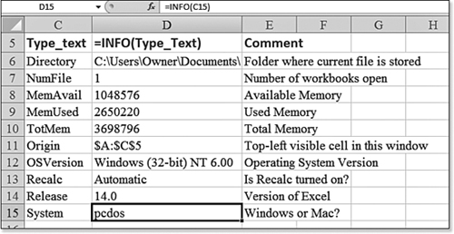
Figure 12.15 shows the results of several variations of the INFO function.
Figure 12.15. A few of the argument values for INFO() still return useful results.
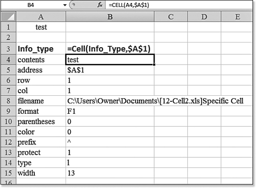
Using the CELL Function
The CELL function can tell you specific information about a specific cell, or it can tell you specific information about the last cell changed in the worksheet.
Again, some of the types of information are a bit dated. For example, the Color argument was written in the day when a cell was either black or possibly red if the value was negative. The Prefix argument is based on when cells could be left-aligned, centered, or right-aligned. Even though Excel has offered several levels of indenting for a decade, the Prefix version of the CELL function does not reveal anything about the indentation level.
Syntax
CELL(info_type,reference)
To use the CELL function, you specify the type of information and optionally a cell reference. If you specify a cell reference, Excel provides information about the cell in the reference. If you leave off the reference, Excel returns information about the last cell changed in the workbook.
The argument info_type is a text value that specifies what type of cell information you want. The following are the possible values of info_type and the corresponding results:
• contents—Returns the value in the upper-left cell in reference.
• address—Returns the address of the first cell in reference, as text. As shown in Cell B5 of Figure 12.16, this is always returned in absolute reference style.
Figure 12.16. The CELL function returns information about a specific cell, in this case, Cell A1.
• row—Returns the row number of the cell in reference.
• col—Returns the column number of the cell in reference.
• filename—Returns the filename as text including the full path of the file that contains reference. If the worksheet that contains reference has not yet been saved, empty text ("") is returned. Interestingly, this argument now also returns the worksheet name if the workbook contains multiple worksheets.
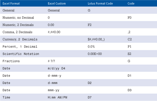
• format—Returns the text value corresponding to the number format of the cell. Returns - at the end of the text value if the cell is formatted in color for negative values. If the cell is formatted with parentheses for positive or all values, () is returned at the end of the text value. The values reported as a format reflect old Lotus 1-2-3 codes. When you format, Excel attempts to convert the current numeric format to an old-style Lotus 1-2-3 formatting code. Table 12.7 shows some examples.
Table 12.7. Custom Codes in Excel and Lotus 1-2-3
• parentheses—Returns 1 if the cell is formatted with parentheses for positive or all values; otherwise, returns 0.
• color—Returns 1 if the cell is formatted in color for negative values; otherwise, returns 0.
• prefix—Returns the text value corresponding to the “label prefix” of the cell as follows:
• Returns a single quotation mark (') if the cell contains left-aligned text.
• Returns double quotation mark (") if the cell contains right-aligned text.
• Returns a caret (^) if the cell contains centered text.
• Returns a backslash () if the cell contains fill-aligned text.
• Returns an empty text ("") if the cell contains anything else.
• protect—Returns 0 if the cell is not locked and 1 if the cell is locked. Remember that by default, all Excel cells start with their locked property set to TRUE. The locked property is taken into account only if protection is enabled. This argument for the CELL function reports a 1 even if protection is not turned on.
Caution
![]()
Be careful with this: It is now possible to change column widths without causing Excel to calculate. You might have to press F9 to have the result of this formula change.
• type—Returns the text value corresponding to the type of data in the cell as follows:
• Returns b for blank if the cell is empty.
• Returns l for label if the cell contains a text constant.
• Returns v for value if the cell contains anything else.
• width—Returns the column width of the cell, rounded to an integer. Each unit of column width is equal to the width of one character in the default font size.
• reference—Is an optional cell reference. If reference is omitted, CELL returns the information about the last changed cell.
Refer back to Figure 12.16, which shows every CELL option for a specific cell: Cell A1.
For additional examples, see Excel Help for the CELL function.
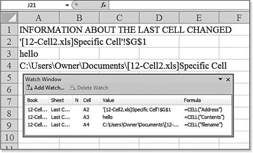
Using CELL to Track the Last Cell Changed
If you leave off the second argument of the CELL function, Excel returns the information about the last cell changed in the workbook.
Follow these steps to create an interesting watch window of the last cells changed:
- In an out-of-the-way spot, enter the formula
=CELL("address"). - Just below this formula, enter the formula
=CELL("Contents"). - Just below that formula, enter the formula
=CELL("filename"). - Select all three of these cells.
- From the Formulas tab, select the Watch Window icon. The Watch Window dialog appears.
- Click the Add Watch button in the Watch Window dialog.
- Because initially, the default file widths are not wide enough to show the complete value, drag the vertical bars between the headings in the watch window so that you can see the complete Value and Formula columns. The other columns for Book, Sheet, and Cell can be made smaller.
The result, as shown in Figure 12.17, is a floating window that always reveals the last changed cell address and contents.
Figure 12.17. The watch window always shows the last cell changed and the value of that cell. Note that as in this case, the last changed cell might be on another worksheet.
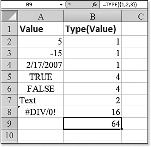
Using TYPE to Determine Type of Cell Value
The final information function is the TYPE function. You use =TYPE(value) to determine whether a value is a number, text, logical, an error value, or an array. Note that dates are treated as numbers.
Syntax
=TYPE(value)
The TYPE function returns a numeric code that tells you about the type of value.
The TYPE function returns the following values:
• 1—For a numeric or date type
• 2—For a text type
• 4—For a logical type
• 16—For an error type
• 64—An array type
Figure 12.18 shows the results for various values in the TYPE function.
Figure 12.18. The TYPE function returns what type of value is specified as an argument.
Examples of Lookup and Reference Functions
The Lookup & Reference icon contains 18 functions. The all-star of this group is the venerable VLOOKUP function, which is one of the most powerful and most used functions in Excel. As database people point out, a lot of work done in Excel should probably be done in Access. The VLOOKUP function allows you to perform the equivalent of a join operation in a database.
This lookup and reference group also includes several functions that seem useless when considered alone. However, when combined, they allow for some very powerful manipulations of data. The examples in the following sections reveal details on how to use the lookup functions and how to combine them to create powerful results.
Using the CHOOSE Function for Simple Lookups
Most lookup functions require you to set up a lookup table in a range on the worksheet. However, the CHOOSE function allows you to specify up to 254 choices right in the syntax of the function. The formula that requires the lookup should be able to calculate an integer from 1 to 254 in order to use the CHOOSE function.
Syntax
CHOOSE(index_num,value1,value2,...)
The CHOOSE value chooses a value from a list of values, based on an index number.
The CHOOSE function takes the following arguments:
• index_num—This specifies which value argument is selected. index_num must be a number between 1 and 254 or a formula or reference to a cell containing a number between 1 and 254:
• If index_num is 1, CHOOSE returns value1; if it is 2, CHOOSE returns value2; and so on.
• If index_num is a decimal, it is rounded down to the next lowest integer before being used.
• If index_num is less than 1 or greater than the number of the last value in the list, CHOOSE returns a #VALUE! error.
• value1,value2,...—These are 1 to 254 value arguments from which CHOOSE selects a value or an action to perform based on index_num. The arguments can be numbers, cell references, defined names, formulas, functions, or text.
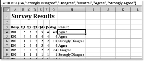
The example in Figure 12.19 shows survey data from a number of respondents. Columns B:F indicate their responses on five measures of your service. Column G calculates an average that ranges from 1 to 5. Say that you want to add words to Column H to characterize the overall rating from the respondent. The following formula is used in Cell H4:
=CHOOSE(G4,"Strongly Disagree","Disagree","Neutral","Agree","Strongly Agree")
Figure 12.19. CHOOSE is great for simple choices where the index number is between 1 and 254.
Using VLOOKUP with TRUE to Find a Value Based on a Range
VLOOKUP stands for vertical lookup. This function behaves differently, depending on the fourth parameter. This section describes using VLOOKUP where you need to choose a value based on a table that contains ranges.
Suppose that you have a list of students and their scores on a test. The school grading scale is based on these ranges:
• 92–100 is an A.
• 85–91 is a B.
• 70–85 is a C.
• 65–69 is a D.
• Below 65 is an F.
Follow these steps to set up a VLOOKUP for this scenario:
- Because in this version of
VLOOKUPyou do not have to list every possible grade, build a table showing the scores where the grading scale changes from one grade to the next. - Although the published grading scale starts with the higher values, your lookup table must be sorted in ascending sequence. This requires a bit of translation as you set up the table. Although the grading scale says below 65 is an F, you need to set up the table to show that an F corresponds to any grade at 0 or above. Therefore, in Cell E2 enter 0, and in Cell F2, enter F.
- Continue building the grading scale in successive rows of Columns E and F. Anything above a 65 is given a D. Anything above 70 is given a C. Note that this is somewhat counterintuitive because it is the opposite order that you would use if you were building a grading scale using nested
IFfunctions. - Ensure that the numeric values are the leftmost column in your lookup table. In Figure 12.20, the lookup table range is E2:F6. When you use
VLOOKUP, Excel searches the first column of the lookup table for the appropriate score.Figure 12.20. The
VLOOKUPformula in Column C finds the correct grade from the table in Columns E and F.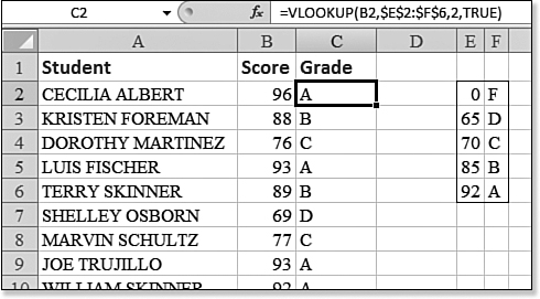
- When using this version of
VLOOKUPwith ranges, sort the list in ascending order. If you are not sure of the proper order, use the Sort command from the Home tab to sort the table. - Because the first argument in the
VLOOKUPfunction is the student’s score, in Cell C2, enter=VLOOKUP(B2,. - Because the next argument is the range of the lookup table, be sure to press the F4 key after typing
E2:F6to change to an absolute reference of$E$2:$F$6. - Ensure that the third argument specifies which column of the lookup table should be returned. Because the letter grade is in the second column of E2:F6, use 2 for the third argument.
- Ensure that the final argument is either
TRUEor simply omitted. This tells Excel that you are using the sorted range variety of lookup. - After you enter the formula in Cell C2, again select Cell C2 and double-click the fill handle to copy the formula down to all students.
Using VLOOKUP with FALSE to Find an Exact Value
In some situations, you do not want VLOOKUP to return a value based on a close match. Instead, you want Excel to find the exact match in the lookup table.
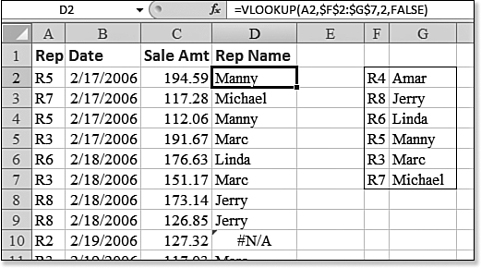
Figure 12.21 shows a table of sales. The original table had just Columns A through C: Rep#, Date, and Sale Amount. Although a data analyst might have all the rep numbers memorized, the manager who is going to see the report prefers to have the rep names on the report.
Figure 12.21. In this case, VLOOKUP needs to find the exact rep number from the table in Columns E and F.
To fill in the rep names from a lookup table, you follow these steps:
- In Columns F and G, enter a table of rep numbers and rep names. Note that it is not important that this table be sorted by the rep number field. It is fine that the table is alphabetical.
- Use
FALSEas the fourth parameter inVLOOKUP. You need to do this because close matches are not acceptable here. If something was sold by a new rep with number R9, you do not want to give credit to the name associated with R8 just because it is a close match. Either Excel finds an exact match and returns the result, or Excel does not give you a result. - For Cell D2, you want Excel to use the rep number in A2, so in Cell D2, enter
=VLOOKUP(A2,. - The lookup table is in
F2:G7, so typeF2:G7and then press the F4 key to make the reference absolute. This allows you to copy the formula in step 7. After pressing F4, type a comma. - In the lookup table, the rep name is in Column 2 of the table, so type
2to specify that you want to return the second column of the lookup table. - Finish the function with
FALSE). Press Ctrl+Enter to accept the formula and keep the cursor in Cell D2. - Double-click the fill handle to copy the formula down to all the rows.
VLOOKUPis a very time-intensive calculation. Having thousands ofVLOOKUPformulas significantly affects your recalculation times. In this particular case, you have successfully added rep names. It would be appropriate to convert these live formulas to their current values. Therefore, press Ctrl+C to copy. Then, from the Home tab, select Paste, Paste Values to convert the formulas to values.- Look through the results. If a sale was credited to a new rep who is not in the table, the name appears as
#N/A. Manually fix these records, if needed.
To recap, the two versions of the VLOOKUP formula behave very differently. VLOOKUP with FALSE as the fourth parameter looks for an exact match, whereas VLOOKUP with TRUE as the fourth parameter looks for the closest (lower) match. In the TRUE version, the lookup table must be sorted. In the FALSE version, the table can be in any sequence. In every case, the key field must be in the left column of the lookup table.
Syntax
VLOOKUP(lookup_value,table_array,col_index_num,range_lookup)
VLOOKUP searches for a value in the leftmost column of a table and then returns a value in the same row from a column you specify in the table. The VLOOKUP function takes the following arguments:
• lookup_value—This is the value to be found in the first column of the table. lookup_value can be a value, reference, or text string.
• table_array—This is the table of information in which data is looked up. You can use a reference to a range such as E2:F9 or a range name such as RepTable.
• col_index_num—This is the column number in table_array from which the matching value must be returned. A col_index_num value of 1 returns the value in the first column in table_array; a col_index_num value of 2 returns the value in the second column in table_array, and so on. If col_index_num is less than 1, VLOOKUP returns the #VALUE! error value; if col_index_num is greater than the number of columns in table_array, VLOOKUP returns the #REF! error value.
• range_lookup—This is a logical value that specifies whether VLOOKUP should find an exact match or an approximate match. If it is TRUE or omitted, an approximate match is returned. In other words, if an exact match is not found, the next largest value that is less than lookup_value is returned. If it is FALSE, VLOOKUP finds an exact match. If one is not found, the error value #N/A is returned. If VLOOKUP cannot find lookup_value and if range_lookup is TRUE, it uses the largest value that is less than or equal to lookup_value. If lookup_value is smaller than the smallest value in the first column of table_array, VLOOKUP returns an #N/A error. If VLOOKUP cannot find lookup_value, and range_lookup is FALSE, VLOOKUP returns an #N/A error.
Using VLOOKUP to Match Two Lists
If Excel is used throughout your company, you undoubtedly have many lists in Excel. People use Excel to track everything. How many times are you faced with a situation in which you have two versions of a list and you need to match them up?
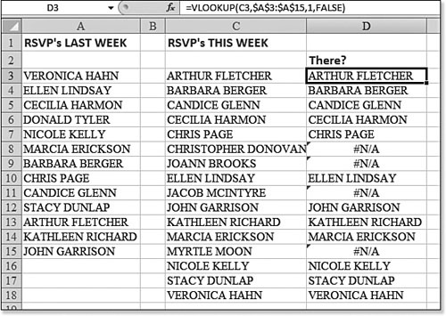
In Figure 12.22, the worksheet has two simple lists. Column A shows last week’s version of who was coming to an event. Column C shows this week’s version of who is coming to an event. Follow these steps if you want to find out quickly if anyone is new:
- Add the heading There? to Cell D2.
- Because the formula in Cell D3 should look at the value in Cell C3 to see if that person is in the original list in Column A, start the formula with
=VLOOKUP(C3,$A$3:$A$15,. - Because your only choice for the column number is to return the first column from the original list, finish the function with
1,FALSE). Then press Ctrl+Enter to accept the formula and stay in Cell D3. - Double-click the fill handle to copy the formula down to all rows.
For any cells where Column D contains a name, it means that the person was on the RSVP list from last week. If the result of the VLOOKUP is #N/A, you know that this person is new since the previous week.
Tip
![]()
If you study the data in Figure 12.22, you will see that three more names are in the Column C list than in the Column A list, yet four people were reported as being new this week. This means that one of the people from last week has dropped off the list. To quickly find who dropped off the list, use the formula =VLOOKUP (A3,$C$3:$C$18,1,FALSE) in B3:B15 to find that Donald Tyler has dropped off the list.
Note that you can also use MATCH to solve this problem.
Figure 12.22. An #N/A error as the result of VLOOKUP tells you that the person is new to the list.
Using COLUMN to Assist with VLOOKUP When Filling a Wide Table
This section discusses some special considerations to keep in mind when you have to retrieve many columns from a table. If you think carefully about the first formula, you can copy the first formula to the entire table quickly.
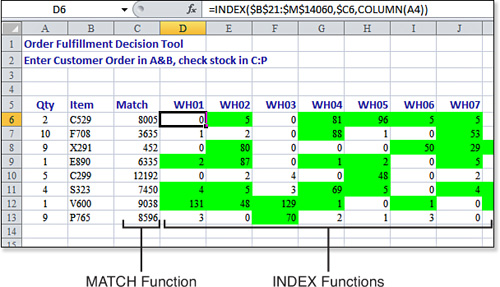
Figure 12.23 shows a table of several hundred SKUs, starting in Row 21. For each SKU, the table contains the inventory of that product on hand in the 12 regional warehouses. Range A6:B13 contains a customer order for various SKUs. You want to build a table to help visualize which warehouse has most of the items in stock. If you find one warehouse that has all the inventory, you can minimize order shipping costs by shipping the entire order from that particular warehouse.
Figure 12.23. The COLUMN function in Row 4 ensures that you can enter the VLOOKUP formula once and copy it to the entire rectangular range.
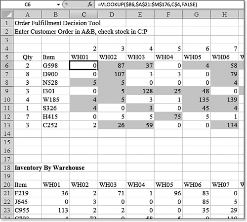
To solve this problem, follow these steps:
- Copy the range of warehouse names from B20:M20 to C5:N5.
- Think about the third argument in the
VLOOKUPfunction. For the formula in Column C, you want to return the second column from the table. For the formula in Column D, you want to return the third column. If you actually enter the 2 in the formula in Column C, then after copying the formula over to D:N, you have to edit the third argument repeatedly. - Create a range above your table, perhaps in Row 4, that contains the numbers 2 through 13. You can then use cells in this row when building the third argument in the formula. In Cell C4, enter the function
=COLUMN(B2). Because Column B is the second column, this formula returns 2. - Select Cell C4. Drag the fill handle to the right to copy the formula over through Column N. The Cell B2 reference is relative, resulting in the formula returning the numbers 2, 3, 4, and so on.
- In Cell C6, enter
=VLOOKUP(B6.When you later copy this formula, you always want the formula to point to Column B, but you want to allow the formula to point to Rows 7, 8, and so on. If you press the F4 key three times, the reference changes to$B6. Type a comma. - Type
A21:M176. Press F4 to change this reference to$A$21:$M$176. Type a comma. - For the third argument, you want to point to the number 2 in Cell C4. You always want this part of the formula to point to Row 4, and you want to allow the column letter to change as the formula is copied to the right. Press the F4 key twice to change the reference to
C$4. - Finish the formula with
,FALSE). Press Ctrl+Enter to accept the formula and stay in Cell C4. - Optionally, add a conditional format to Cell C4 to highlight the cell if this formula is true:
=C6>=$A6. - Double-click the fill handle to copy the formula to
C4:C13. - Drag the fill handle from the corner of
C13to the right until you have filled in the formula in the range ofC:N.
The result is a table that shows the current inventory for each item, by warehouse. If you added the conditional formatting in step 9, you can quickly see which warehouses can fulfill most of the order.
Although having the COLUMN function in Row 4 allows you to visually understand the example better, you can eliminate Row 4 and rewrite the formula in Cell C6 as =VLOOKUP($B6,$A$21:$M$176, COLUMN(B1),FALSE).
Syntax
COLUMN(reference)
The COLUMN function returns the column number of a given reference. This function takes the argument reference, which is the cell or range of cells for which you want the column number. If reference is omitted, it is assumed to be the reference of the cell in which the COLUMN function appears.
If reference is a range of cells, and if COLUMN is entered as a horizontal array, COLUMN returns the column numbers of reference as a horizontal array. In this case, reference cannot refer to multiple areas.
Using HLOOKUP for Horizontal Lookup Tables
HLOOKUP stands for horizontal lookup. This function is similar to VLOOKUP.
HLOOKUP operates in two distinct manners, based on the fourth parameter. If the fourth parameter is the value FALSE, then HLOOKUP is looking for an exact match in the top row of the table. This is fine when you are looking up product codes, customer numbers, or any other discrete bits of information.
However, if the fourth parameter is the value TRUE or is omitted, HLOOKUP is treating the first row of the table as a sorted range of values. Excel looks for the closest lower value than the one you specified. This is fine when you are trying to determine in which range a value belongs.
Syntax
HLOOKUP(lookup_value,table_array,row_index_num,range_lookup)
The HLOOKUP function searches for a value in the top row of a table. When the value is found, HLOOKUP returns a value from a particular row in the column. This function takes the following arguments:
• lookup_value—This is a value to be found in the first row of the table. lookup_value can be a value, a reference, or a text string.
• table_array—This is a table of information in which data is looked up. You use a reference to a range or a range name. The values in the first row of table_array can be text, numbers, or logical values. If range_lookup is TRUE, the values in the first row of table_array must be placed in ascending order such as ..., -2, -1, 0, 1, 2,...; A–Z; or FALSE, TRUE. Otherwise, HLOOKUP may not give the correct value. If range_lookup is FALSE, table_array does not need to be sorted. The search is not case-sensitive: Uppercase and lowercase text are equivalent.
• row_index_num—This is the row number in table_array from which the matching value is returned. A row_index_num of 1 returns the first row value in table_array, a row_index_num of 2 returns the second row value in table_array, and so on. If row_index_num is less than 1, HLOOKUP returns a #VALUE! error; if row_index_num is greater than the number of rows in table_array, HLOOKUP returns a #REF! error.
• range_lookup—This is a logical value that specifies whether you want HLOOKUP to find an exact match or an approximate match. If it is TRUE or omitted, an approximate match is returned. In other words, if an exact match is not found, the next largest value that is less than lookup_value is returned. If it is FALSE, HLOOKUP finds an exact match. If one is not found, the error #N/A is returned.
Even though you are probably familiar with sorting a list from top to bottom, most people rarely sort a list from left to right. If you are using the TRUE version of HLOOKUP, make sure that your table is sorted from left to right by the top row. To sort data from left to right, follow these steps:
- Select your range of data. In Figure 12.24, this is G3:L8.
Figure 12.24. The table in F:L is horizontal, so you use the
HLOOKUPfunction.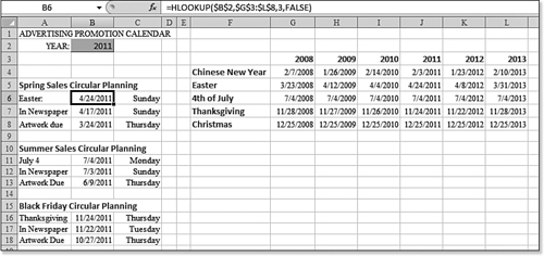
- From the Home tab, select the Sort & Filter drop-down. The Sort dialog appears.
- In the Sort dialog, click the Options button. The Sort Options dialog appears.
- In the Sort Options dialog, select Sort Left to Right. Click OK to close the Sort Options dialog.
- In the Sort dialog, choose to sort by Row 3. Click OK to sort.
Figure 12.24 shows a tool used by the advertising department of a retail store. The store runs annual promotions for certain holidays. The table in F3:L8 tells the days for holidays in each of several years.
The advertising manager knows that the store wants to run a sale circular the Sunday before the holiday and that the art department needs the material 24 days before the ad is to run. By changing the year in Cell B2, the advertising manager can create a new schedule for each year. To help the advertising manager, follow these steps:
- Ensure that the formula for each holiday starts as
=HLOOKUP($B$2,. This tells Excel to use the year found in Cell B2 as the value to look up. - Ensure that the lookup table is in
$G$3:$L$8. Excel looks through the first row of this table to find the matching year. - When the matching column is found, you want Excel to return the date for Easter. Although this is in Row 5 of the worksheet, it is in the third row of the table, so ensure that the third parameter for the function is 3.
- Your years are already sorted left to right, but if you use a value of
TRUEfor the fourth parameter, this causes problems in the year 2014, so make the fourth parameterFALSE. Ensure that the formula in Cell B6 is=HLOOKUP($B$2,$G$3:$L$8,3,FALSE). - Copy this formula to Cell B11 and edit the formula to change the third parameter from
3to4.
Using the MATCH Function to Locate the Position of a Matching Value
At first glance, MATCH seems like a function that would rarely be useful. MATCH returns the relative position of an item in a range that matches a specified value in a specified order. You use MATCH instead of one of the lookup functions when you need the position of an item in a range instead of the item itself.
Suppose that your manager asks, “Can you tell me on which row I would find this value?” The manager wants to know the value or some piece of data on that record. However, the manager rarely wants to know that XYZ is found on the 111th relative row within the Range A99:A11432.
MATCH comes in handy in several instances. In the first instance, consider a situation in which you are using VLOOKUP to find whether an item is in a list. In this case, you do not care what value is returned. You are either interested in seeing if a valid value is returned, meaning that the entry is in the old list, or if an #N/A is returned, meaning that the entry is new. In this case, using MATCH is a slightly faster way to achieve the same result.
Another handy way to use MATCH is in conjunction with the INDEX function. MATCH has two features that make it more versatile than VLOOKUP.MATCH allows for wildcard matches. MATCH also allows for a search based on an exact match, based on the number just below the value, or based on a value greater than or equal to the lookup value. This third option is not available in the VLOOKUP or HLOOKUP functions.
Syntax
MATCH(lookup_value,lookup_array,match_type)
The MATCH function returns the relative position of an item in a column of values. It is useful for determining if a certain value exists in a list.
The MATCH function takes the following arguments:
• lookup_value—This is the value you use to find the value you want in a table. lookup_value can be a value, which is a number, text, or logical value or a cell reference to a number, text, or logical value.
• lookup_array—This is a contiguous range of cells that contains possible lookup values. lookup_array can be an array or an array reference.
• match_type—This is the number -1, 0, or 1. Note that you can use TRUE instead of 1 and FALSE instead of 0. match_type specifies how Microsoft Excel matches lookup_value with values in lookup_array. If match_type is 1, MATCH finds the largest value that is less than or equal to lookup_value. lookup_array must be placed in ascending order, such as ... -2, -1, 0, 1, 2,...; A–Z; or FALSE, TRUE. If match_type is 0, MATCH finds the first value that is exactly equal to lookup_value. lookup_array can be in any order. If match_type is -1, MATCH finds the smallest value that is greater than or equal to lookup_value. lookup_array must be placed in descending order, such as TRUE, FALSE; Z–A; or ...2, 1, 0, -1, -2,.... If match_type is omitted, it is assumed to be 1.
MATCH returns the position of the matched value within lookup_array, not the value itself. For example, MATCH("b",{"a","b","c"},0) returns 2, the relative position of b within the array {"a","b","c"}.
MATCH does not distinguish between uppercase and lowercase letters when matching text values.
If MATCH is unsuccessful in finding a match, it returns an #N/A error.
If match_type is 0 and lookup_value is text, lookup_value can contain the wildcard characters asterisk (*) and question mark (?). An asterisk matches any sequence of characters; a question mark matches any single character.
Using MATCH to Compare Two Lists
You may face situations in which you have two versions of a list, and you need to match them up.
In Figure 12.25, the worksheet has two simple lists. Column A shows last week’s list. Column C shows this week’s version of the list. You want to find out quickly which items are new. Here’s how you do it:
- Add the heading There? to Cell D2.
- Because the formula in Cell D3 looks at the value in Cell C3 to see if that value is in the original list in Column A, start the formula with
=MATCH(C3,$A$3:$A$11,. - Because you want an exact match, use 0 as the third parameter. Finish the function with
a ). Press Ctrl+Enter to accept the formula and stay in Cell C3. - Double-click the fill handle to copy the formula down to all rows.
Figure 12.25. MATCH operates slightly more quickly than VLOOKUP and achieves the same result in this special case where you are trying to figure out whether a value is in another list.

For any cells where Column D contains a number, it means that the entry was on the original list from last week. If the result of MATCH is #N/A, you know that this item is new since the previous week.
Using INDEX and MATCH for a Left Lookup
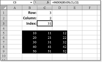
INDEX is another function that does not immediately seem to have many great uses. In its basic form, INDEX returns the cell from a particular row and column of a rectangular range.
As shown in Figure 12.26, using =INDEX(B5:D9,3,2) seems like a needlessly complicated way to refer to Cell C7.
Figure 12.26. On its own, INDEX is not a particularly useful function.
However, in the previous section you learned about a function that searches through a range and tells you the position of the match within the range. Finding the position of a match is not very useful. However, finding the position of a match is very useful when used inside of the INDEX function.
In Figure 12.27, a customer number is entered in Cell A1. The customer lookup table appears in Columns F, G, and H. The main problem is that the customer table does not have the customer number on the left side.
Figure 12.27. This combination of INDEX and MATCH allows you to look up data that is to the left of a key field.
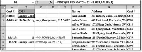
In many cases, you would copy Column H to Column E and use Column E as the key of the table. However, the table in F:H is likely to be repopulated every day from a web query or an OLAP query. Therefore, it might become monotonous to move the data after every refresh. The solution is to use a combination of INDEX and MATCH. Here’s what you do:
- Use the formula
=MATCH(B1,H2:H89,0)to search through Column H to find the row with the customer number that matches the one in Cell B1. In this case, C593 is in Row 12, which is the 11th row of the table. - Be sure to use exactly the same shape range as the first argument in the INDEX function:
=INDE X(F2:F89,WhichRow,WhichColumn)searches through the customer names in Column F. - For the second parameter of the
INDEXfunction, specify the relative row number. This information was provided by theMATCHfunction in step 1. - Ensure that the third parameter of the
INDEXfunction is the relative column number. Because the Range F2:F89 has only one column, this is either 1 or it can simply be omitted. - Putting the formula together, the formula in Cell B2 is
=INDEX(F2:F89,MATCH(B1,H 2:H89,0),1).
Syntax
INDEX(array,row_num,[column_num])
The INDEX function will return the value at the intersection of a particular row and column within a range.
The INDEX function takes the following arguments:
• array—This is a range of cells or an array constant. If array contains only one row or column, the corresponding row_num or column_num argument is optional. If array has more than one row and more than one column, and if only row_num or column_num is used, INDEX returns an array of the entire row or column in array.
• row_num—This selects the row in array from which to return a value. If row_num is omitted, then column_num is required.
• column_num—This selects the column in array from which to return a value. If column_num is omitted, then row_num is required.
If both the row_num and column_num arguments are used, INDEX returns the value in the cell at the intersection of row_num and column_num.
If you set row_num or column_num to 0, INDEX returns the array of values for the entire column or row, respectively. To use values returned as an array, you use the INDEX function as an array formula in a horizontal range of cells for a row and in a vertical range of cells for a column. To enter an array formula, you press Ctrl+Shift+Enter.
row_num and column_num must point to a cell within array; otherwise, INDEX returns a #REF! error.
Using MATCH and INDEX to Fill a Wide Table
The lookup functions VLOOKUP, HLOOKUP, and MATCH can be very processor-intensive when the lookup table contains hundreds of thousands of rows.
Back in Figure 12.23, Excel had to do 96 VLOOKUP functions. However, after Excel figured out the position of Item G598 in the lookup table for Cell C6, it had to go back through exactly the same steps for Cell D6, E6, F6, G6, and so on. You made Excel find exactly the same item 12 times, which is a very slow process.
If the recalculation times are taking too long, you should consider using one MATCH per row to find the relative row number and then using 12 speedy INDEX functions to fill in the values in that row. Figure 12.28 illustrates a problem where you can use this trick. In this case, the list of inventory items is 14,000 rows. Here’s what you do:
- Copy the range of warehouse names from B20:M20 to D5:O5.
- In Cell C6, enter
=MATCH(B6,$A$21:$A$14060,0). This formula finds an exact match for C529. The answer 8005 means that product C529 is on the 8,005th relative row of the lookup range. - Copy the formula in Cell C6 to C6:C13.
- As you build the
INDEXfunction, be careful that the array range encompasses the same rows used in theMATCHfunction. Start the formula in Cell D6 as=INDEX($B$21:$M$14060. Make sure to press F4 to make this reference absolute. - Make the next argument the relative row number within the lookup range. This is the value from Column C, so use
$C6. If you typeC6and then press the F4 key three times, Excel adds the dollar sign before theCinC6. - Add the final argument, the column number. For the first warehouse, this would be Column 1. However, rather than typing a 1 for the formula, use
COLUMN(A1). This allows you to copy the formula to the rest of the range. Finish the formula with a parenthesis. The final formula is=IND EX($B$21:$M$14060,$C6,COLUMN(A4)). Note that it is not important if you useCOLUMN(A1), COLUMN(A4),orCOLUMN(A10000). All of those will return the number 1. - Optionally, add a conditional format to Cell D6 to highlight the cell if this formula evaluates to
TRUE: =D6>=$A6. - Copy the formula from Cell D6 to D6:O13.
Figure 12.28. This performs eight relatively slow MATCH functions and then 96 relatively fast INDEX functions.
Performing Many Lookups with LOOKUP
Even Excel Help tells you to avoid the old LOOKUP function. However, LOOKUP can do one useful trick that VLOOKUP and HLOOKUP cannot do—it can process many lookups in one single array formula. LOOKUP can also deal with a lookup range that is vertical and a return range that is horizontal, or vice-versa.
The next section looks at the common use of LOOKUP and how it contrasts with VLOOKUP or HLOOKUP.
Syntax
LOOKUP(lookup_value, array)
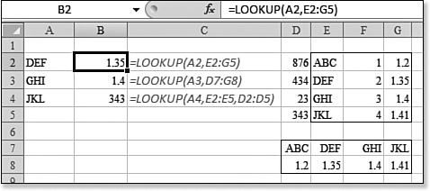
In this case, LOOKUP is acting similar to VLOOKUP or HLOOKUP. Excel examines the height and width of the array. If the array has more rows than columns, Excel assumes you are doing a VLOOKUP and looks through the first column of the array for the lookup value. If the array has more columns than rows, Excel assumes you are doing an HLOOKUP and looks through the first row of the array for the lookup value.
In this syntax of LOOKUP, Excel always returns the value from the last column or row of the array. In Figure 12.29, the formula in B2 is returning a value from Cell G3. Because the array is described as E2:G5, Excel automatically returns a value from the final column of E2:G5. Because the array is four rows and three columns, Excel assumes you want the equivalent of VLOOKUP instead of HLOOKUP. In Cell B3, the lookup array is D7:G8. Because this array is wider than it is tall, Cell B3 does the equivalent of an HLOOKUP.
Figure 12.29. The quirky LOOKUP function decided to do a VLOOKUP or HLOOKUP depending on the shape of the lookup array.
In addition, LOOKUP always performs a range lookup, similar to leaving off the FALSE as the fourth parameter of VLOOKUP or HLOOKUP. For this reason, your lookup array must always be sorted.
If you do not want to return a value from the last column of the array, you can specify two vectors in the alternative form of the syntax discussed in the next section.
Syntax
LOOKUP(lookup_value, lookup_vector, result_vector)
In this version of the LOOKUP function, you specify vectors that are either one row tall or one column wide. This version allows you to do a lookup similar to VLOOKUP where the result field is to the left of the key field. In Cell B4 of Figure 12.29, the result vector is to the left of the lookup vector.
So far, everything about LOOKUP can be accomplished using VLOOKUP, HLOOKUP, or INDEX and MATCH. However, a useful trick makes LOOKUP better than those other functions: You can ask Excel to look up many values at one time, provided that you do the following:
- Press Ctrl+Shift+Enter to accept the formula..
- Enclose the
LOOKUPin a wrapper function such asSUMto summarize all the results from the function.
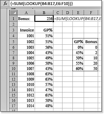
In Figure 12.30, a series of invoices appear in Rows 4 through 17. A GP% (gross profit percentage) is associated with each invoice. The sales rep will earn a bonus depending on the GP% of each invoice as shown in E6:F10. Instead of calculating a bonus for each row, you can calculate a bonus for all the rows at once. The formula in B1 of Figure 12.30 specifies an array of B4:B17 as the lookup value. This causes Excel to perform the LOOKUP 14 times, once for each value in the Range B4:B17. The formula wraps the LOOKUP results in a SUM function to add up all the bonus results. To calculate correctly, you must hold down Ctrl+Shift while pressing Enter after typing this formula.
Figure 12.30. Unlike VLOOKUP and HLOOKUP, the aging LOOKUP function can process many lookups in a single array formula.
Using Functions to Describe the Shape of a Contiguous Reference
Four functions can be used to identify the location and shape of a contiguous range:
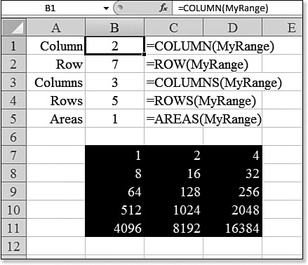
• COLUMN(reference)—This returns the column number of the upper-left corner of a reference, using numbers from 1 to 16,384. If reference is omitted, the function returns the column number of the cell where the formula is entered.
• ROW(reference)—This returns the row number of the upper-left corner of the reference, using numbers from 1 to 1,045,876. If reference is omitted, the function returns the row number of the cell where the formula is entered.
• COLUMNS(reference)—This returns the number of columns in a reference. In this case, reference must be a single contiguous range.
• ROWS(reference)—This returns the number of rows in a reference. Again, reference must be a single contiguous range.
Figure 12.31 displays the ROW, COLUMN, ROWS, and COLUMNS functions of a named range. The range occupies the black cells in B7:D11.
Figure 12.31. These functions describe the location and shape of a range.
Using AREAS and INDEX to Describe a Range with More Than One Area
All the functions listed in the preceding section fail if the reference describes a noncontiguous range. However, you can check for that condition by using the AREAS function.
Syntax
AREAS(reference)
This function returns the number of contiguous ranges in a reference. The argument reference usually refers to a named range.
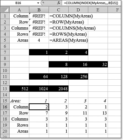
In Figure 12.32, MyAreas is a defined name that describes the cells in black. In Rows 1 through 4, all the traditional functions fail with #REF! errors because the reference contains more than one contiguous range.
Figure 12.32. To describe a reference with multiple contiguous ranges, you have to use the reference form of the INDEX function.
Syntax
INDEX(reference,row_num,column_num,area_num)
If you need to determine the location and shape of each contiguous range, do so one area at a time. A second syntax for the INDEX function returns a reference to one specific area of a reference. This syntax includes the following arguments:
• reference—Reference to one or more cell ranges. If you are entering a nonadjacent range for the reference, enclose the reference in parentheses. If each area in reference contains only one row or column, the row_num or column_num argument, respectively, is optional. For example, for a single row reference, you use INDEX(reference,column_num).
• row_num—The number of the row in reference from which to return a reference.
• column_num—The number of the column in reference from which to return a reference.
• area_num—Selects a range in reference from which to return the intersection of row_num and column_num. The first area selected or entered is numbered 1, the second is 2, and so on. If area_num is omitted, INDEX uses area 1. For example, if reference describes the Cells (A1:B4,D1:E4,G1:H4), then area_num 1 is the Range A1:B4, area_num 2 is the Range D1:E4, and area_num 3 is the Range G1:H4.
After reference and area_num have selected a particular range, row_num and column_num select a particular cell: row_num 1 is the first row in the range, column_num 1 is the first column, and so on. The reference returned by INDEX is the intersection of row_num and column_num.
If you set row_num or column_num to 0, INDEX returns the reference for the entire column or row, respectively.
row_num, column_num, and area_num must point to a cell within reference; otherwise, INDEX returns a #REF! error. If row_num and column_num are omitted, INDEX returns the area in reference specified by area_num.
The result of the INDEX function is a reference, and it is interpreted as such by other formulas. Depending on the formula, the return value of INDEX may be used as a reference or as avalue. For example, the formula CELL("width",INDEX(A1:B2,1,2)) is equivalent to CELL("width",B1). The CELL function uses the return value of INDEX as a cell reference. On the other hand, a formula such as 2*INDEX(A1:B2,1,2) translates the return value of INDEX into the number in Cell B1.
Using this version of INDEX, you can build formulas that work on one particular area in a named range. Here’s how you do it:
- In B15:E15, enter the numbers 1 through 4. These correspond to the four areas in
MyAreas. - When you build the
INDEXfunction, you want Excel to return a reference to the entire rows and columns of the first area of the range, so use=INDEX(MyAreas,,,1)to return such a reference. - Instead of using
1for theareasargument ofINDEX, use=INDEX(MyAreas,,,B$15). - Enter the formula
=COLUMN(INDEX(MyAreas,,,B$15))in Cell B16 to define the starting column of area 1 ofMyAreas. - Copy the formula from step 4 to B17:B20. Edit each function to change
COLUMNtoROW,COLUMNS,ROWS, andAREAS. - Copy B17:B20 to Columns C, D, and E.
The result, as shown in Figure 12.32, includes four sets of formulas in B16:E20 that completely describe the four areas of the named range MyAreas.
Using Numbers with OFFSET to Describe a Range
The language of Excel is numbers. There are functions that count the number of entries in a range. There are functions that can tell you the numeric position of a looked-up value. You may know that a particular value is found in Row 20, but what if you want to perform calculations on other cells in Row 20?
The OFFSET function handles this very situation. You can use OFFSET to describe a range using mostly numbers. OFFSET is flexible: It can describe a single cell, or it can describe a rectangular range.
Although INDEX can return a single cell from a rectangular range, it has limitations. If you specify C5:Z99 as the range for an INDEX function, you can select only cells below and/or to the right of C5. The OFFSET function can move up and down or left and right from the starting cell, which is C5.
Syntax
OFFSET(reference,rows,cols,height,width)
The OFFSET function returns a reference to a range that is a given number of rows and columns from a given reference.
The OFFSET function takes the following arguments:
• reference—This is the reference from which you want to base the offset. reference must be a reference to a cell or range of adjacent cells; otherwise, OFFSET returns a #VALUE! error.
• rows—This is the number of rows, up or down, that you want the upper-left cell to refer to. Using 5 as the rows argument, for example, specifies that the upper-left cell in the reference is five rows below reference. Rows can be positive, which means below the starting reference, or negative, which means above the starting reference.
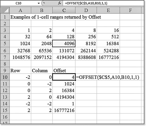
• cols—This is the number of columns to the left or right that you want the upper-left cell of the result to refer to. For example, using 5 as the cols argument specifies that the upper-left cell in the reference is five columns to the right of reference. cols can be positive, which means to the right of the starting reference, or negative, which means to the left of the starting reference. If rows and cols offset reference over the edge of the worksheet, OFFSET returns a #REF! error. Figure 12.33 demonstrates various combinations of rows and cols from a starting cell of Cell C5.
Figure 12.33. These OFFSET functions return a single cell that is a certain number of rows and columns away from Cell C5.
• height—This is the height, in number of rows that you want the returned reference to be. Height must be a positive number.
• width—This is the width, in number of columns that you want the returned reference to be. Width must be a positive number. If height or width is omitted, Excel assumes it is the same height or width as reference.
OFFSET allows you to specify a reference. It does not move any cell. It does not change the selection. It is just a numeric way to describe a reference. OFFSET can be used in any function that is expecting a reference argument.
Excel Help provides a trivial example of =SUM(OFFSET(C2,1,2,3,1)), which sums E3:E5. However, this example is silly because no one would ever write such a formula! If you were to write such a formula, you would just write =SUM(E3:E5) instead. The power of OFFSET comes when at least one of the four numeric arguments is calculated by the COUNT function or a lookup function.
In Figure 12.34, you can use COUNT(A5:A99) to count how many entries are in Column A. If you assume that there are no blanks in the range of data, you can use the COUNT result as the height argument in OFFSET to describe the range of numbers. Here’s what you do:
- There is nothing magic about the reference, so write it as
=OFFSET(A5,. - Do not move the starting position any rows or columns from Cell A5. The starting position is A5, so you always use 0 and 0 for rows and columns. Therefore, the formula is now
=OFFSET(A5,0,0,. - If you want to include only the number of entries in the list, use
COUNT(A5:A999)as the height of the range. The formula is now=OFFSET(A5,0,0,COUNT(A5:A999),. - The width is one column, so make the function
=OFFSET(A5,0,0,COUNT(A5:A999),1). - Use your
OFFSETfunction anywhere that you would normally specify a reference. You can use=SUM(OFFSET(A5,0,0,COUNT(A5:A999),1))or specify that formula as the series in a chart. This creates a dynamic chart that grows or shrinks as the number of entries changes.
Figure 12.34. Every argument except height is hard-coded in these functions. The height argument comes from a COUNT function to allow the range to expand as more entries are added.

For a more complex example of OFFSET, examine Figure 12.35, which shows several yearly tables starting in Cell C8. Each month of the table contains from one to five entries. The person using this spreadsheet will select a year and a month from Cells E1 and E2. The goal is to find information about the entries for that particular month and year. Here’s how you do it:
- Have the formula in Cell I1 find the starting row for the particular year, using the
MATCHfunction shown in Cell J1. - Have the formula in Cell I2 find the column for the chosen month, using the
MATCHfunction shown in Cell J2. - Build the
OFFSETfunction to describe the range for that month and year. You know that it starts in the row in I1 and thecolumnin I2. If you make thereferenceCell A1, then Row 15 is 14 rows below A1. Therefore, use=OFFSET(A1,I1-1,. - The starting column is in Cell I2. Column 8 is seven columns to the right of A1. Therefore, you now use
=OFFSET(A1,I1-1,I2-1. - The structure of the worksheet allows for up to five entries per month, arranged down a row. Thus,
heightis5andwidthis1. Use the following formula to describe the possible range for the month:=OFFSET(A1,I1-1,I2-1,5,1). This is good enough to use forMIN,MAX,SUM, and so on. - To chart the data, figure out the exact height. Use the
=COUNT(OFFSET(A1,I1-1,I2-1,5,1))formula in Cell I3 to count the number of entries for the month. - Use the formula
=OFFSET(A1,I1-1,I2-1,I3,1)to describe the exact month. Add additional formulas in I4:I6 to figure out the minimum, maximum, and sum of those cells.
Figure 12.35. Even with a poorly designed database spreadsheet, various combinations of OFFSET can locate and total cells for a specific month.
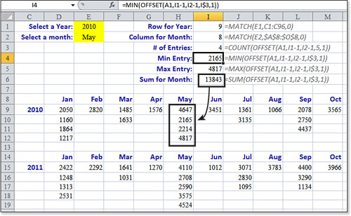
The OFFSET function initially seems intimidating, especially in light of the example you just walked through. Remember that for useful results from OFFSET, you usually replace one or more of the final four arguments with a calculation.
Using ADDRESS to Find the Address for Any Cell
If someone asks you for the cell address for the cell in Row 5, Column 5, you could probably come up with E5 quickly. What if someone asks you for the cell address of the cell in Row 26, Column 26? This is Z26. Again, you should come up with this if you know there are 26 letters in the alphabet.
If someone asks you to calculate the address of Row 2 and Column 30, you have to divide 30 by 26 to learn that the result is 1 with a remainder of 4. This could lead you to conclude the cell address is the first letter of the alphabet—A—and the fourth letter of the alphabet—D—to come up with AD2.
This type of calculation becomes far more complex with 16,384 columns. For example, how would you calculate the address for Row 2 of Column 14123?
Fortunately, Excel provides the ADDRESS function to convert any intersection of row and column number to an address. =ADDRESS(2,14123) returns the text of $TWE$2.
Syntax
ADDRESS(row_num,column_num,abs_num,a1,sheet_text)
The default version of ADDRESS returns the cell address as an absolute address with both dollar signs. There are optional parameters to control this behavior:
• row_num—This is the row number to use in the cell reference.
• column_num—This is the column number to use in the cell reference.
• abs_num—This specifies the type of reference to return. If it is 1 or omitted, the returned address has both dollar signs and is absolute. If it is 2, the row is held absolute, but the column is relative. If it is 3, the row is relative and the column is absolute. If it is 4, the address is relative, with no dollar signs.
• a1—This is a logical value that specifies the A1 or R1C1 reference style. If a1 is TRUE or omitted, ADDRESS returns an A1-style reference; if it is FALSE, ADDRESS returns an R1C1-style reference.
• sheet_text—This is text that specifies the name of the worksheet to be used as the external reference. If sheet_text is omitted, no sheet name is used.
Figure 12.36 shows eight ways to describe one cell, depending on the various combinations of absolute and A1 arguments.
Figure 12.36. ADDRESS can return a cell address in A1 or R1C1 style.
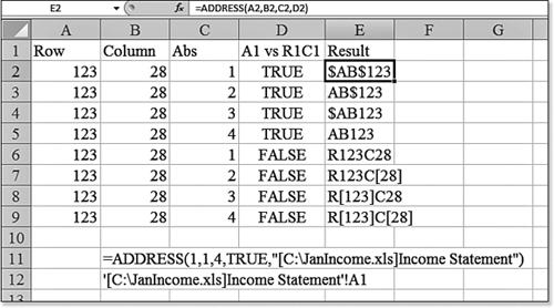
The sheet_text argument is interesting. It is difficult to remember the arcane rules for when to use apostrophes and where the exclamation point needs to go in an address. If you specify sheet_text as the name of a worksheet or use the style [book_name]SheetName, Excel builds the proper reference. Cell B11 in Figure 12.36 shows the result from an ADDRESS function that builds a reference to another workbook.
Using INDIRECT to Build and Evaluate Cell References On-the-Fly
The INDIRECT function is deceivingly powerful. Consider this trivial example: In Cell A1, enter the text B2. In Cell B2, enter a number. In cell C3, enter the formula, =INDIRECT(A1). Excel will return the number that you entered in cell B2 in cell C3. The INDIRECT function looks in cell A1 and expects to find something that is a valid cell or range reference. It then looks in that address to return the answer for the function.
The reference text can be any text that you can string together using various text functions. This allows you to create complex references that dynamically point to other sheets or to other open workbooks.
The reference text can also be a range name. You could have a validation list box where someone selects a value from a list. If you have predefined a named range that corresponds to each possible entry on the list, INDIRECT can point to the various named ranges on-the-fly.
When you use traditional formulas, even absolute formulas, there is a chance that someone might insert rows or columns that will move the reference. If you need a formula to always point to Cell J10, no matter how someone rearranges the worksheet, you can use =INDIRECT("J10") to handle this.
Syntax
INDIRECT(ref_text,a1)
The INDIRECT function returns the reference specified by a text string.
The INDIRECT function takes the following arguments:
• ref_text—This is a reference to a cell that contains an A1-style reference, an R1C1-style reference, a name defined as a reference, or a reference to a cell as a text string. If ref_text is not a valid cell reference, INDIRECT returns a #REF! error. If ref_text refers to an external workbook, the other workbook must be open. If the source workbook is not open, INDIRECT returns a #REF! error.
• a1—This is a logical value that specifies what type of reference is contained in the cell ref_text. If a1 is TRUE or omitted, ref_text is interpreted as an A1-style reference. If a1 is FALSE, ref_text is interpreted as an R1C1-style reference.
Figure 12.37 is a monthly worksheet in a workbook that has 12 similar sheets. In each worksheet, the data headings are in Row 6, and the invoices appear for some number of rows, starting in Row 7. Each worksheet has a total for the month in Cell D2.
Figure 12.37. You can add a year-to-date formula to all sheets.
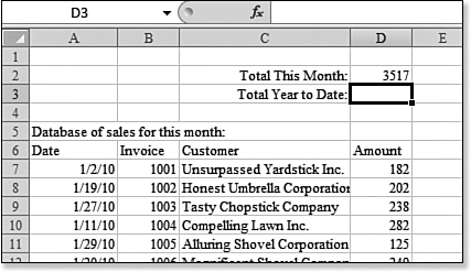
In this example, you want to add a year-to-date total in Cell D3 on each worksheet. This is fairly difficult to do without VBA. Many VBA books include a user-defined function to describe the previous sheet in a workbook. However, this function will fail if you send the workbook to someone who disables macros or her computer. Instead, you can solve this problem with clever use of text functions and the INDIRECT function. To do so, follow these steps:
- Select the Jan worksheet.
- Shift+click the Dec worksheet to put all 12 sheets in Group mode.
- In Cell A1, enter the formula =A7. This adds the first date as a title for the worksheet.
- Format Cell A1 with the custom format
mmmm, yyyy. This causes the date to appear as January, 2010. - Right-click the Jan tab name and select Ungroup Sheets.
- Enter
=D2as the year-to-date formula in Cell D3 of the Jan tab. - On the Feb worksheet, build a text formula that returns the name of the previous month. The quest becomes how to build a formula that looks like
=Jan!D3. - Jan is a three-letter abbreviation for any date in the month of January. Therefore, enter a January date in a cell and format the cell with the custom number format mmm, so that the result is the word
Jan. - The
TEXTfunction takes a number or date and displays it using a specific custom number format, so on the February sheet, use=TEXT(A1,"mmm"), which results in the valueFeb. This is close. If you can find a way to get the name of the previous month, the problem will be solved. - The value in Cell A1 is a live date. You can use date math to calculate a different date, such as the date one month earlier. Use the
DATE(year,month,day)function to return a date in the previous month. For the year parameter, useYEAR(A1). For the month parameter, useMONTH(A1)–1. For the day parameter, useDAY(A1). The formula=DATE(YEAR(A1),MONTH(A1)–1,1)returns a date that is the first of the previous month. - Combining steps 9 and 10 into a single formula, use
=TEXT(DATE(YEAR(A1),MONTH(A1)–1,1),"MMM")to return the value ofJanon the Feb worksheet,Febon the March worksheet, and so on. - Use the generic formula
=TEXT(DATE(YEAR(A1),MONTH(A1)–1,1),"MMM")&"!D3"to build the reference. - Select the Feb worksheet. Shift+click the Dec worksheet to place these 11 worksheets in Group mode. In Cell D3, enter this formula:
=INDIRECT(TEXT(DATE(YEAR(A1),MONTH(A1)–1,1),"mmm")&"!D3")+D2. - Right-click any sheet tab and select Ungroup to take the workbook out of Group mode.
The result, as shown in Figure 12.38, is a formula on the last 11 worksheets that automatically pulls the year-to-date total from the previous worksheet and adds it to the current worksheet total.
Figure 12.38. Cell D4 dynamically builds a text formula to reference the previous sheet, and then INDIRECT evaluates the formula.
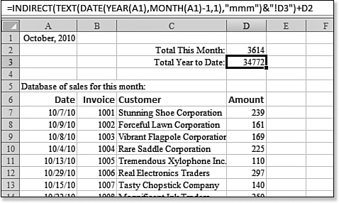
Using the HYPERLINK Function to Quickly Add Hyperlinks
Excel enables you to add a hyperlink by using the Excel interface. On the Insert tab, select the Hyperlink icon. Next, you specify text to appear in the cell and the underlying address. Building links in this way is easy, but it is tedious to build them one at a time. If you have hundreds of links to add, you can add them quickly by using the HYPERLINK function.
Syntax
HYPERLINK(link_location,friendly_name)
The HYPERLINK function creates a shortcut that opens a document stored on your hard drive, a network server, or on the Internet.
The HYPERLINK function takes the following arguments:
• link_location—This is the URL address on the Internet. It could also be a path, filename, and location in another file. For example, you could link to "[C:filesJan2007. xls]!Sheet1!A15". Note that link_location can be a text string enclosed in quotes or a cell that contains the link.
• friendly_name—This is the underlined text or numeric value that is displayed in the cell. friendly_name is displayed in blue and is underlined. If friendly_name is omitted, the cell displays the link_location value as the jump text. friendly_name can be a value, a text string, a name, or a cell that contains the jump text or value. If friendly_name returns an error (for example, #VALUE!), the cell displays the error instead of the jumptext.
Note
![]()
Note that Excel does not check whether the link location is valid at the time you created the link. If the link is not valid when someone clicks it, the person encounters an error.
Tip
![]()
It is difficult to select a cell that contains a HYPERLINK function. If you click the cell, Excel attempts to follow the hyperlink. Instead, you should click a cell near the cell and then use the arrow keys to move into the cell.
Figure 12.39 shows a list of web pages in Column A. Column B contains the titles of those web pages. To quickly build a table of hyperlinks, you use =HYPERLINK(A2,B2) in Cell C2 and copy the formula down the column. After the hyperlinks are created, you can copy Column C and use Paste Values on Column C. You are then free to delete Columns A and B.
Figure 12.39. The formulas in Column C allow you to create hundreds of hyperlinks in seconds.
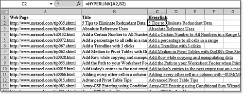
Using the TRANSPOSE Function to Formulaically Turn Data
With many people using Excel in a company, there are bound to be different usage styles from person to person. Some people build their worksheets horizontally, and other people build their worksheets vertically. For example, in Figure 12.40, the monthly totals stretch horizontally across Row 80. However, for some reason, you need these figures to be arranged going vertically down from Cell B84.
Figure 12.40. Turning C80:N80 into a vertical range is called transposing the data.
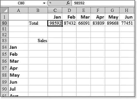
The typical method is to copy C80:N80 and then use Home, Paste, Transpose. This copies a snapshot of the totals in Row 80 to a column of data.
This is fine if you only need a snapshot of the totals. However, what if you want to see the totals continually updated in Column B? Excel provides the TRANSPOSE function for such situations.
Because the function returns several answers, you need to use special care when entering the formula. Here’s how:
- Note that C80:N80 contains 12 cells.
- Select an identical number of cells starting in B84. Select B84:B95.
- Even though you have 12 cells selected, type the formula
=TRANSPOSE(C80:N80)as if you had only one cell selected. - To tell Excel that this is a special type of formula called an
array formula, hold down Ctrl+Shift while you press Enter.
Excel shows the formula surrounded by curly braces in the formula bar. This is one single formula entered in 12 cells. Therefore, you cannot delete or change one cell in the range. If you want to change the formula, you need to delete all 12 cells in B84:B95 in a single command.
Figure 12.41 shows a TRANSPOSE function that occupies 12 cells.
Figure 12.41. One TRANSPOSE function occupies 12 cells, from B84:B95.
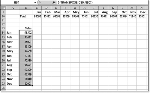
Syntax
TRANSPOSE(array)
The TRANSPOSE function transposes a vertical range into a horizontal array, or vice versa.
The argument array is an array or a range of cells on a worksheet that you want to transpose. The transposition of an array is accomplished by using the first row of the array as the first column of the new array, the second row of the array as the second column of the new array, and so on.
Using the RTD Function and COM Add-ins to Retrieve Real-Time Data
Third-party applications are available to send streaming real-time data to an Excel spreadsheet. They became very popular with stock day traders back in the late 1990s. If you have one of these COM add-ins installed on your system, you can set up a formula to retrieve real-time data from the COM add-in by using the RTD function. If you have such a COM add-in installed, the vendor of the add-in should provide sample workbooks with RTD functions already in place.
Syntax
RTD(progid,server,topic1,[topic2],...)
The RTD function returns real-time data from a program that supports COM automation.
The RTD function takes the following arguments:
• progid—This is the name of the Program ID of a registered COM automation add-in that has been installed on the local computer. You need to enclose the name in quotation marks.
• server—This is name of the server where the add-in should be run. If there is no server and the program is run locally, leave this argument blank.
• topic1, topic2,...—These are 1 to 28 parameters that together represent a unique piece of real-time data.
Using GETPIVOTDATA to Retrieve One Cell from a Pivot Table
You might turn to this book to find out how to use most of the functions. However, for the GETPIVOTDATA function, you are likely to turn to this book to find out why the function is being automatically generated for them.
Suppose that you have a pivot table on a worksheet. You should click outside the pivot table. Next, you type an equal sign and then with the mouse, click one of the cells in the data area of the pivot table. Although you might expect this to generate a formula such as =E9, instead, Excel puts in the formula =GETPIVOTDATA("Sales",$B$5,"Customer","Astonishing Glass Company","Region","West"), as shown in Figure 12.42.
Figure 12.42. Excel inserts this strange function in the worksheet.
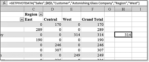
This function is annoying. As you copy the formula down to more rows, the function keeps retrieving sales to Astonishing Glass in the West region. By default, Excel is generating this function instead of a simple formula such as =E9. This happens whether you use the mouse or the arrow keys to specify the cell in the formula.
To avoid this behavior, you can type the entire formula by manually typing it on the keyboard. Typing =E9 in a cell forces Excel to create a relative reference to Cell E9. You are then free to copy the formula to other cells.
There is also a way to turn off this behavior permanently:
- Select a cell inside an active pivot table.
- The Pivot Table Tools tabs appears. Select the Options tab. From the PivotTable group, select the Options drop-down and then select the Generate GetPivotData icon (see Figure 12.43). The behavior turns off.
Figure 12.43. You can disable the
GETPIVOTDATAfunction option.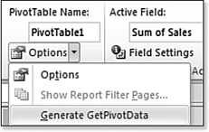
- Enter formulas by using the mouse, arrow keys, or keyboard without generating the
GETPIVOTDATAfunction.
Microsoft made GETPIVOTDATA the default behavior because the function is pretty cool. Now that you have learned how to turn off the behavior, you might want to understand exactly how it works in case you ever need to use the function.
Syntax
GETPIVOTDATA(data_field,pivot_table,field1,item1,field2,item2,...)
The GETPIVOTDATA function returns data stored in a pivot table report. You can use GETPIVOTDATA to retrieve summary data from a pivot table report, provided that the summary data is visible in the report. This function takes the following arguments:
• data_field—This is the name, enclosed in quotation marks, for the data field that contains the data you want to retrieve.
• pivot_table—This is a reference to any cell, range of cells, or named range of cells in a pivot table report. This information is used to determine which pivot table report contains the data you want to retrieve.
• field1, item1, field2, item2,...—These are 1 to 14 pairs of field names and item names that describe the data you want to retrieve. The pairs can be in any order. Field names and names for items other than dates and numbers are enclosed in quotation marks. For OLAP pivot table reports, items can contain the source name of the dimension as well as the source name of the item.
Calculated fields or items and custom calculations are included in GETPIVOTDATA calculations.
If pivot_table is a range that includes two or more pivot table reports, data is retrieved from whichever report was created in the range most recently.
If the field and item arguments describe a single cell, the value of that cell is returned, regardless of whether it is a string, a number, an error, and so on.
If an item contains a date, the value must be expressed as a serial number or populated by using the DATE function so that the value is retained if the spreadsheet is opened in a different locale. For example, an item referring to the date March 5, 1999, could be entered as 36224 or DATE(1999,3,5). Times can be entered as decimal values or by using the TIME function.
If pivot_table is not a range in which a pivot table report is found, GETPIVOTDATA returns #REF!. If the arguments do not describe a visible field, or if they include a page field that is not displayed, GETPIVOTDATA returns #REF!.
Examples of Database Functions
If you were a serious data analyst in the 1980s and the early 1990s, you would have been enamored with the database functions. I personally used @DSUM every hour of my work life for many years. It was one of the most powerful weapons in any spreadsheet arsenal. Combined with a data table, the DSUM, DMIN, DMAX, and DAVERAGE functions got a serious workout when users performed data analysis in a spreadsheet.
Then, in 1993, Microsoft Excel added the pivot table to the Data menu in Excel. Pivot tables changed everything. Those powerful database functions seemed tired and worn out. Since that day in 1993, I had never used DSUM again until I created the example described in the following section. As far as I knew, the database functions had been living in a cave in South Carolina.
Maybe it is like the nostalgia of finding a box of photos of an old girlfriend, but I realize that the database functions are still pretty powerful. Customers whined enough to have Microsoft add AVERAGEIF to the COUNTIF and SUMIF arsenal. This was unnecessary: Customers could have done this easily by setting up a small criteria range and using DAVERAGE.
Eleven of the 12 database functions are similar. DSUM, DAVERAGE, DCOUNT, DCOUNTA, DMAX, DMIN, DPRODUCT, DSTDEV, DSTDEVP, DVAR, and DVARP all perform the equivalent operation of their non-D equivalents, but they allow for complex criteria to include records that meet certain criteria.
To save you the hassle of looking up the confusing few, DCOUNT counts numeric cells, and DCOUNTA counts nonblank cells. DSTDEV and DVAR calculate the standard deviation and variance of a sample of a population. DSTDEVP and DVARP calculate the standard deviation and variance of the entire population. The 12th database function, DGET, has the same arguments, but it acts a bit differently, as explained later in this chapter.
Using DSUM to Conditionally Sum Records from a Database
There are three arguments to every database function. It is very easy to get your first DSUM working. The criteria argument is the one that offers vast flexibility. The following section explains the syntax for DSUM. The syntax for the other 11 database functions is identical tothis.
Syntax
DSUM(database,field,criteria)
The DSUM function will add records from one field in a data set, provided that the records meet some criteria that you specify.
The DSUM function takes the following arguments:
• database—This is the range of cells that make up the list or database, including the heading row. A database is a list of related data in which rows of related information are records and columns of data are fields. In Figure 12.44, the database is the 5,000 rows of data located at A23:I5024.
Figure 12.44. A simple criteria range specifies to limit DSUM to only records for Best Paint Inc. as a customer.
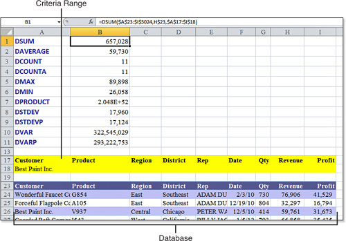
• field—This indicates which column is used in the function. You have three options when specifying a field:
• You can point to the cell with the field name such as H23 for Revenue.
• You can include the word Revenue as the field argument.
• You can use the number 8 to indicate that Revenue is the eighth field in the database.
• criteria—This is the range of cells that contains the conditions specified. You can use any range for the criteria argument. The criteria range typically includes at least one column label and at least one cell below the column label for specifying a condition for the column. You can also use the computed criteria discussed in “Using the Miracle Version of the Criteria Range” later in this chapter. Learning how to create powerful criteria ranges allows you to unlock the powerful potential of the database functions. Several examples are provided in the following sections.
Note
![]()
To conserve space, the remaining examples in the following sections show only the DSUM result. You can compare the various results to the $657,028 of revenue for the current example.
Creating a Simple Criteria Range for Database Functions
Although a criteria range needs only one field heading from the database, it is just as easy to copy the entire set of headings to a blank section of the worksheet. In Figure 12.44, for example, the headings in A17:I17, along with at least one additional row, create a criteria range.
In Figure 12.44, you see results of the 11 database functions for a simple criteria where the customer is Best Paint Inc. Each formula specifies a database of $A$23:$I$5024. The field is H23, which is the heading for Revenue. The criteria range is A17:I18. In this example, the criteria range could have easily been A17:A18, but the A17:I18 form allows you to enter future criteria without respecifying the criteria range.
Using a Blank Criteria Range to Return All Records
This is a trivial example, but if the second row of the criteria range is completely blank, the database function returns the total of all rows in the data set. As shown in Figure 12.45, this is $256 million. This is equivalent to using the SUM function.
Figure 12.45. If the second row of the criteria is blank, the result reflects all rows.
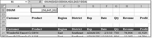
Using AND to Join Criteria
Many people using SUMIF in Excel 2003 and earlier are likely to want to know how to conditionally sum based on two conditions. This is simple to do with DSUM. If two criteria are placed on the same row of the criteria range, they are joined by an AND. In Figure 12.46, forexample, the $123,275 is the sum of records where the customer is Best Paint and the product is V937.
Figure 12.46. When two criterion are on the same line, they are joined by an AND function; rows must meet both criteria to be included in the DSUM.
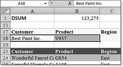
Using OR to Join Criteria
When two criteria are placed on separate rows of the criteria range, they are joined by an OR function. In Figure 12.47, the $2.1 million represents records for either Improved Radio Traders or Best Paint.
Figure 12.47. When two criteria are on different rows, they are joined by an OR function; rows can meet either criteria to be included in the DSUM.
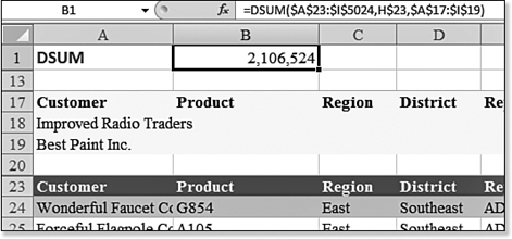
You can use OR to join criteria from different fields. The criteria range in Figure 12.48 shows a Region value of West joined by an OR with a District value of Texas. This pulls a superset of all the West records plus just the Texas records which happen to fall in the central region.
Figure 12.48. The criteria to be joined with OR can be in separate columns.
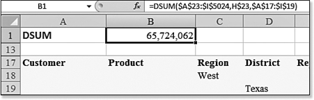
Using Dates or Numbers as Criteria
The example in Figure 12.49 finds records with a date in 2015 and with revenue under $50,000. This data set does not contain any records from 2016, so you only need to check for items beyond 2014. The criteria in F18 for the date could have used any of these formats:
>12/31/2014
>=1/1/2015
>31-Dec-2014
Figure 12.49. Using dates or numbers in criteria.
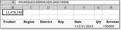
Using the Miracle Version of a Criteria Range
Using the criteria ranges in the preceding examples, you could easily build any complex criteria with multiple AND or OR operators.
However, this could get complex. Imagine if you wanted to pull all the records for five specific customers and five specific products. You would have to build a criteria range that is 26 rows tall. Basically, the first row is the headings for customer and product. The second row indicates that you want to see records for Customer1 and Product1. The third row indicates that you want to see records for Customer1 and Product2. The fourth row indicates that you want to see records for Customer1 and Product3. The seventh row indicates Customer2 and Product1. The 26th row indicates Customer5 and Product5.
If you need to pull the records for seven customers and seven products from five districts, your criteria range would grow to 246 rows tall and will probably never finish calculating.
There is a miraculous version of the criteria range that completely avoids this problem. Here’s how it works:
• The criteria range consists of a range that is two cells tall and one or more cells wide.
• Contrary to instructions in Excel help, the top cell of the criteria range cannot contain a field heading. The top cell must be blank or contain anything which does not match the database header row. For example, you could put a heading of “Computed Criteria.”
• The second row in the criteria range can contain any formula that evaluates to TRUE or FALSE. This formula must point to cells in the first data row of the database. The formula can be as complex as you wish, with AND, OR, VLOOKUP, NOT, and MATCH; it can contain any combination of functions.
For a simple example, suppose you want to find records that match 1 of 15 customers. You copy the customers to K24:K38. In the second row of the criteria field, write the formula =NOT(ISNA(MATCH (A24,$K$24:$K$38,0))). This formula does a MATCH on the first customer in the database to see if it is in the list in K. The ISNA and NOT functions make sure that the criteria cell returns a TRUE when the customer is 1 of the 15 customers.
Very quickly and without complaint, Excel compares the 5,000 rows of your database with this complex formula, and the DSUM produces the correct value, as shown in Figure 12.50.
Figure 12.50. The formula version of the criteria range is rare but incredibly powerful.
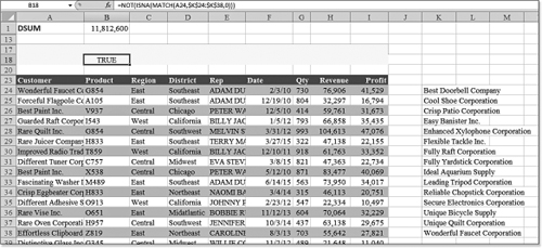
![]() To watch a video of DSUM with this criteria range, search for “Excel In Depth 12” at YouTube.
To watch a video of DSUM with this criteria range, search for “Excel In Depth 12” at YouTube.
Using the DGET Function
The DGET function returns a single cell from a database. The problem is that this function is picky. If your criteria range matches zero records, DGET returns a #VALUE error. If your criteria range returns more than one row, DGET returns a #NUM! error.
To have DGET work, you need to write a criteria record that causes one and only one row to be evaluated as TRUE.
Syntax
DGET(database,field,criteria)
The DGET function returns a single cell matching criteria from a data set.
The DGET function takes the following arguments:
• database—This is the range of cells that make up the list or database. A database is a list of related data in which rows of related information are records and columns of data are fields. The first row of the list contains labels for each column.
• field—This indicates which column is used in the function. Field can be given as text, with the column label enclosed between double quotation marks, such as "Age" or "Yield", or as a number that represents the position of the column within the list (for example, 1 for the first column, 2 for the second column, and so on).
• criteria—This is the range of cells that contains the conditions you specify. You can use any range for the criteria argument, as long as it includes at least one column label and at least one cell below the column label for specifying a condition for the column.
Excel in Practice: Using DSUM with a Data Table
If you do not want to use a pivot table, you can do a crosstab analysis by using a combination of the DSUM function and the Data Table command. The Data Table command works best when a problem is set up with two variables. In the DSUM function, you might have two variables defined in the criteria range.
To set up a two-variable table using the DSUM function, follow these steps:
- Ensure that the upper-left corner of the table is a formula that relies on at least two variables. In Figure 12.51, Cell B1 contains a
DSUMthat relies on the criteria ranges in A17:I18.Figure 12.51. The Data Table dialog requires two cells.
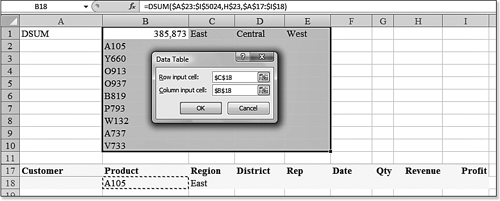
- Down the left side of the table, arrange a list of values that should be substituted for one variable. In this example, the column contains a list of products that will eventually be substituted into Cell B18.
- Across the top row of the table, arrange a list of values that should be substituted for the other variable. In this example, the row contains a list of regions that will eventually be substituted into Cell C18.
- Select the range for the table. This selection should include the formula as the upper-left corner cell. It should also include the column and row of headings.
- From the Data tab, select What-if Analysis, Data Table. The Data Table dialog appears, asking for twocells.
- For the row input cell, enter the cell where the regions should be substituted. In this case, it is Cell C18 in the criteria range.
- For the Column input cell, enter the cell where the values down the left column will be substituted. In this case, it is Cell B18 in the criteria range. The complete dialog box should look as shown in Figure 12.52.
Figure 12.52. The resulting table provides a crosstab analysis similar to that in a pivot table.
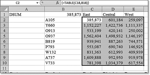
The result is a crosstab analysis that shows the DSUM for every combination of product and region. Excel actually creates a TABLE array function to produce the answers. This is a live formula: If you change the product names or regions, the cells inside the table recalculate.