3
State‐Space Models for Identification
3.1 Introduction
State‐space models are easily generalized to multichannel, nonstationary, and nonlinear processes [1–23]. They are very popular for model‐based signal processing primarily because most physical phenomena modeled by mathematical relations naturally occur in state‐space form (see [15] for details). With this motivation in mind, let us proceed to investigate the state‐space representation in a more general form to at least “touch” on its inherent richness. We start with continuous‐time systems and then proceed to the sampled‐data system that evolves from digitization followed by the purely discrete‐time representation – the primary focus of this text.
3.2 Continuous‐Time State‐Space Models
We begin by formally defining the concept of state [1]
. The state of a system at time ![]() is the “minimum” set of variables (state variables) along with the input sufficient to uniquely specify the dynamic system behavior for all
is the “minimum” set of variables (state variables) along with the input sufficient to uniquely specify the dynamic system behavior for all ![]() over the interval
over the interval ![]() . The state vector is the collection of state variables into a single vector. The idea of a minimal set of state variables is critical, and all techniques to define them must ensure that the smallest number of “independent” states have been defined in order to avoid possible violation of some important system theoretic properties [2,3]. In short, one can think of states mathematically as simply converting an
. The state vector is the collection of state variables into a single vector. The idea of a minimal set of state variables is critical, and all techniques to define them must ensure that the smallest number of “independent” states have been defined in order to avoid possible violation of some important system theoretic properties [2,3]. In short, one can think of states mathematically as simply converting an ![]() th‐order differential equation into a set of
th‐order differential equation into a set of ![]() ‐first‐order equations – each of which is a state variable. From a systems perspective, the states are the internal variables that may not be measured directly, but provide the critical information about system performance. For instance, measuring only the input/output voltages or currents of an integrated circuit board with a million embedded (internal) transistors – the internal voltages/currents would be the unmeasured states of this system.
‐first‐order equations – each of which is a state variable. From a systems perspective, the states are the internal variables that may not be measured directly, but provide the critical information about system performance. For instance, measuring only the input/output voltages or currents of an integrated circuit board with a million embedded (internal) transistors – the internal voltages/currents would be the unmeasured states of this system.
Let us consider a general deterministic formulation of a nonlinear dynamic system including the output (measurement) model in state‐space form (continuous‐time)1

for ![]() ,
, ![]() , and
, and ![]() the respective
the respective ![]() ‐state,
‐state, ![]() ‐output, and
‐output, and ![]() ‐input vectors with corresponding system (process), input, measurement (output), and feedthrough functions. The
‐input vectors with corresponding system (process), input, measurement (output), and feedthrough functions. The ![]() ‐dimensional system and input functions are defined by
‐dimensional system and input functions are defined by ![]() and
and ![]() , while the
, while the ![]() ‐dimensional output and feedthrough functions are given by
‐dimensional output and feedthrough functions are given by ![]() and
and ![]() .
.
In order to specify the solution of the ![]() th‐order differential equations completely, we must specify the above‐noted functions along with a set of
th‐order differential equations completely, we must specify the above‐noted functions along with a set of ![]() ‐initial conditions at time
‐initial conditions at time ![]() and the input for all
and the input for all ![]() . Here
. Here ![]() is the dimension of the “minimal” set of state variables.
is the dimension of the “minimal” set of state variables.
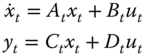
If we constrain the state‐space representation to be linear in the states, then we obtain the generic continuous‐time, linear, time‐varying state‐space model given by
where ![]() ,
, ![]() ,
, ![]() and the respective system, input, output, and feedthrough matrices are:
and the respective system, input, output, and feedthrough matrices are: ![]() ,
, ![]() ,
, ![]() , and
, and ![]() .
.
An interesting property of the state‐space representation is to realize that these models represent a complete generic form for almost any physical system. That is, if we have an RLC circuit or a mass‐damper‐spring (MCK) mechanical system, their dynamics are governed by the identical set of differential equations – only their coefficients differ. Of course, the physical meaning of the states is different, but this is the idea behind state‐space – many physical systems can be captured by this generic form of differential equations, even though the systems are physically different.
Systems theory, which is essentially the study of dynamic systems, is based on the study of state‐space models and is rich with theoretical results exposing the underlying properties of the system under investigation. This is one of the major reasons why state‐space models are employed in signal processing, especially when the system is multivariable, having multiple inputs and multiple outputs (MIMO). Next we develop the relationship between the state‐space representation and input/output relations – the transfer function.
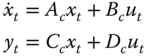
For this development, we constrain the state‐space representation above to be a linear time‐invariant (LTI) state‐space model given by
where ![]() ,
, ![]() ,
, ![]() , and
, and ![]() their time invariant counterparts with the subscript, “
their time invariant counterparts with the subscript, “![]() ,” annotating continuous‐time matrices.
,” annotating continuous‐time matrices.
This LTI model corresponds the constant coefficient differential equation solutions, which can be solved using Laplace transforms. Taking the Laplace transform2 of these equations and solving for ![]() , we have that
, we have that
where ![]() is the identity matrix. The corresponding output is
is the identity matrix. The corresponding output is
From the definition of transfer function (zero initial conditions), we have the desired result

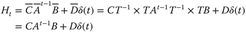
Taking the inverse Laplace transform of this equation gives us the corresponding impulse response matrix of the LTI‐system as [1]
So we see that the state‐space representation enables us to express the input–output relations in terms of the internal variables or states. Note also that this is a multivariable representation compared to the usual single‐input‐single‐output (SISO) (scalar) systems models that frequently appear in the signal processing literature.
Now that we have the multivariable transfer function representation of our LTI system, we can solve the state equations directly using inverse transforms to obtain the time‐domain solutions. First, we simplify the notation by defining the Laplace transform of the state transition matrix or the so‐called resolvent matrix of systems theory [ 1 , 3 ] as
with
Therefore, the state transition matrix is a critical component in the solution of the state equations of an LTI system given by
and we can rewrite the transfer function matrix as
with the corresponding state‐input transfer matrix given by
Taking the inverse Laplace transformation gives the time‐domain solution
or

with the corresponding output solution

Revisiting the continuous‐time system of Eq. 3.12 and substituting the matrix exponential for the state transition matrix gives the LTI solution as
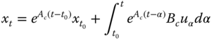
and the corresponding measurement system
In general, the continuous state transition matrix satisfies the following properties: [ 1 , 2 ]
 is uniquely defined for
  (Unique)
 (Identity)
 satisfies the matrix differential equation:
(3.16)
satisfies the matrix differential equation:
(3.16)
 (Semi‐Group)
 (Inverse)
Thus, the transition matrix plays a pivotal role in LTI systems theory for the analysis and prediction of the response of LTI and time‐varying systems [2]
. For instance, the poles of an LTI govern important properties such as stability and response time. The poles are the roots of the characteristic (polynomial) equation of ![]() , which are found by solving for the roots of the determinant of the resolvent, that is,
, which are found by solving for the roots of the determinant of the resolvent, that is,
Stability is determined by assuring that all of the poles lie within the left half of the ![]() ‐plane. Next we consider the sampled‐data state‐space representation.
‐plane. Next we consider the sampled‐data state‐space representation.
3.3 Sampled‐Data State‐Space Models
Sampling a continuous‐time system is commonplace with the advent of high‐speed analog‐to‐digital converters (ADC) and modern computers. A sampled‐data system lies somewhere between the continuous analog domain (physical system) and the purely discrete domain (stock market prices). Since we are strictly sampling a continuous‐time process, we must ensure that all of its properties are preserved. The well‐known Nyquist sampling theorem precisely expresses the required conditions (twice the highest frequency) to achieve “perfect” reconstruction of the process from its samples [15] .
Thus, if we have a physical system governed by continuous‐time dynamics and we “sample” it at given time instants, then a sampled‐data model can be obtained directly from the solution of the continuous‐time state‐space model. That is, we know from Section 3.2 that

where ![]() is the continuous‐time state transition matrix that satisfies the matrix differential equation of Eq. 3.16, that is,
is the continuous‐time state transition matrix that satisfies the matrix differential equation of Eq. 3.16, that is,
Sampling this system such that ![]() over the interval
over the interval ![]() , then we have the corresponding sampling interval defined by
, then we have the corresponding sampling interval defined by ![]() . Note this representation need not necessarily be equally‐spaced – another important property of the state‐space representation. Thus, the sampled solution becomes
. Note this representation need not necessarily be equally‐spaced – another important property of the state‐space representation. Thus, the sampled solution becomes

and therefore from the differential equation of Eq. 3.16 , we have the solution

where ![]() is the sampled‐data state transition matrix – the critical component in the solution of the state equations enabling us to calculate state evolution in time. Note that for an LTI sampled‐data system, the state‐transition matrix is
is the sampled‐data state transition matrix – the critical component in the solution of the state equations enabling us to calculate state evolution in time. Note that for an LTI sampled‐data system, the state‐transition matrix is ![]() where
where ![]() is the sampled‐data system (process) matrix.
is the sampled‐data system (process) matrix.
If we further assume that the input excitation is piecewise constant (![]() ) over the interval
) over the interval ![]() , then it can be removed from under the superposition integral in Eq. 3.18 to give
, then it can be removed from under the superposition integral in Eq. 3.18 to give

Under this assumption, we can define the sampled‐data input transmission matrix as

and therefore the sampled‐data state‐space system with equally or unequally sampled data is given by

Computationally, sampled‐data systems pose no particular problems when care is taken, especially since reasonable approximation and numerical integration methods exist [19]. This completes the discussion of sampled‐data systems and approximations. Next we consider the discrete‐time systems.
3.4 Discrete‐Time State‐Space Models
Discrete state‐space models, the focus of subspace identification, evolve in two distinct ways: naturally from the problem or from sampling a continuous‐time dynamical system. An example of a natural discrete system is the dynamics of balancing our own checkbook. Here the state is the evolving balance given the past balance and the amount of the previous check. There is “no information” between time samples, so this model represents a discrete‐time system that evolves naturally from the underlying problem. On the other hand, if we have a physical system governed by continuous‐time dynamics, then we “sample” it at given time instants. So we see that discrete‐time dynamical systems can evolve from a wide variety of problems both naturally (checkbook) or physically (circuit). In this text, we are primarily interested in physical systems (physics‐based models), so we will concentrate on sampled systems reducing them to a discrete‐time state‐space model.
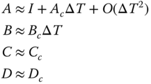
We can use a first‐difference approximation and apply it to the general LTI continuous‐time state‐space model of Eq. 3.2 to obtain a discrete‐time system, that is,

Solving for ![]() , we obtain
, we obtain

Recognizing that the first‐difference approximation is equivalent to a first‐order Taylor series approximation of ![]() gives the discrete system, input, output, and feedthrough matrices as
gives the discrete system, input, output, and feedthrough matrices as
The discrete, linear, time‐varying state‐space representation is given by the system or process model as
and the corresponding discrete output or measurement model as
where ![]() are the respective
are the respective ![]() ‐state,
‐state, ![]() ‐input,
‐input, ![]() ‐output and
‐output and ![]() are the (
are the (![]() )‐system, (
)‐system, (![]() )‐input, (
)‐input, (![]() )‐output, and (
)‐output, and (![]() )‐feedthrough matrices.
)‐feedthrough matrices.
The state‐space representation for (LTI), discrete systems is characterized by constant system, input, output, and feedthrough matrices, that is,
![]()
and is given by the LTI system

The discrete system representation replaces the Laplace transform with the ![]() ‐transform defined by the transform pair:
‐transform defined by the transform pair:

Time‐invariant state‐space discrete systems can also be represented in input/output or transfer function form using the ![]() ‐transform to give
‐transform to give

where recall “adj” is the matrix adjoint (transpose of the cofactor matrix) and “det” is the matrix determinant.
We define the characteristic equation or characteristic polynomial of the ![]() ‐dimensional system matrix
‐dimensional system matrix ![]() as
as
with roots corresponding to the poles of the underlying system that are also obtained from the eigenvalues of ![]() defined by
defined by

for ![]() is the
is the ![]() th system pole.
th system pole.
Taking inverse ![]() ‐transforms of Eq. 3.29, we obtain the discrete impulse (or pulse) response matrix as
‐transforms of Eq. 3.29, we obtain the discrete impulse (or pulse) response matrix as
for ![]() the Kronecker delta function.
the Kronecker delta function.
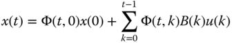
The solution to the state‐difference equations can easily be derived by induction [3] and is given by

where ![]() is the discrete‐time state‐transition matrix. For time‐varying systems, it can be shown (by induction) that the state‐transition matrix satisfies
is the discrete‐time state‐transition matrix. For time‐varying systems, it can be shown (by induction) that the state‐transition matrix satisfies
while for time‐invariant systems the state‐transition matrix is given by
The discrete state‐transition matrix possesses properties analogous to its continuous‐time counterpart, that is,
 is uniquely defined (Unique)
 (Identity)
 satisfies the matrix difference equation:
(3.34)
satisfies the matrix difference equation:
(3.34)
 (Semi‐Group)
 (Inverse)
3.4.1 Linear Discrete Time‐Invariant Systems
In this section, we concentrate on the discrete LTI system that is an integral component of the subspace identification techniques to follow. Here we develop a compact vector–matrix form of the system input/output relations that will prove useful in subsequent developments.
For a discrete LTI system, we have that the state transition matrix becomes

The discrete LTI solution of Eq. 3.33 is therefore
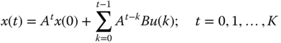
with the measurement or output system given by

Expanding this relation further over ![]() ‐samples and collecting terms, we obtain
‐samples and collecting terms, we obtain

where ![]() is the observability matrix and
is the observability matrix and ![]() is a Toeplitz matrix [15]
.
is a Toeplitz matrix [15]
.
Shifting these relations in time (![]() ) yields
) yields

leading to the vector input/output relation
Catenating these ![]() ‐vectors (
‐vectors (![]() ) of Eq. 3.39 to create a batch‐data (block Hankel) matrix over the
) of Eq. 3.39 to create a batch‐data (block Hankel) matrix over the ![]() ‐samples, we can obtain the “data equation,” that is, defining the block matrices as
‐samples, we can obtain the “data equation,” that is, defining the block matrices as


and, therefore, we have the vector–matrix data equation that relates the system model to the data (input and output matrices)
This expression represents the fundamental relationship for the input–state–output of an LTI state‐space system. Next we discuss some of the pertinent system theoretic results that will enable us to comprehend much of the subspace realization algorithms to follow.
3.4.2 Discrete Systems Theory
In this section we investigate the discrete state‐space model from a systems theoretic viewpoint. There are certain properties that a dynamic system must possess in order to assure a consistent representation of the dynamics under investigation. For instance, it can be shown [2] that a necessary requirement of a measurement system is that it is observable, that is, measurements of available variables or parameters of interest provide enough information to reconstruct the internal variables or states.
Mathematically, a system is said to be completely observable, if for any initial state, say ![]() , in the state‐space, there exists a finite
, in the state‐space, there exists a finite ![]() such that knowledge of the input
such that knowledge of the input ![]() and the output
and the output ![]() is sufficient to specify
is sufficient to specify ![]() uniquely. Recall that the linear state‐space representation of a discrete system is defined by the following set of equations:
uniquely. Recall that the linear state‐space representation of a discrete system is defined by the following set of equations:
with the corresponding measurement system or output defined by
Using this representation, the simplest example of an observable system is one in which each state is measured directly, therefore, and the measurement matrix ![]() is a
is a ![]() matrix. In order to reconstruct
matrix. In order to reconstruct ![]() from its measurements
from its measurements ![]() , then from the measurement system model,
, then from the measurement system model, ![]() must be invertible. In this case, the system is said to be completely observable; however, if
must be invertible. In this case, the system is said to be completely observable; however, if ![]() is not invertible, then the system is said to be unobservable.
is not invertible, then the system is said to be unobservable.
The next level of complexity involves the solution to this same problem when ![]() is a
is a ![]() matrix, then a pseudo‐inverse must be performed instead [ 1
, 2
]. In the general case, the solution gets more involved because we are not just interested in reconstructing
matrix, then a pseudo‐inverse must be performed instead [ 1
, 2
]. In the general case, the solution gets more involved because we are not just interested in reconstructing ![]() , but
, but ![]() over all finite values of
over all finite values of ![]() ; therefore, we must include the state model, that is, the dynamics as well.
; therefore, we must include the state model, that is, the dynamics as well.
With this motivation in mind, we now formally define the concept of observability. The solution to the state representation is governed by the state‐transition matrix, ![]() , where recall that the solution of the state equation is [3]
, where recall that the solution of the state equation is [3]
Therefore, premultiplying by the measurement matrix, the output relations are

or rearranging we define

The problem is to solve this resulting equation for the initial state; therefore, multiplying both sides by ![]() , we can infer the solution from the relation
, we can infer the solution from the relation
Thus, the observability question now becomes under what conditions can this equation uniquely be solved for ![]() ? Equivalently, we are asking if the null space of
? Equivalently, we are asking if the null space of ![]() is
is ![]() . It has been shown [ 2
,4] that the following
. It has been shown [ 2
,4] that the following ![]() observability Gramian has the identical null space, that is,
observability Gramian has the identical null space, that is,

which is equivalent to determining that ![]() is nonsingular or rank
is nonsingular or rank ![]() .
.
Further assuming that the system is LTI then over a finite time interval for ![]() for
for ![]() leads to the
leads to the ![]() observability matrix [4]
given by
observability matrix [4]
given by
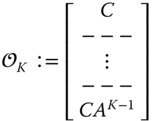
Therefore, a necessary and sufficient condition for a system to be completely observable is that the rank of ![]() or
or ![]() must be
must be ![]() . Thus, for the LTI case, checking that all of the measurements contain the essential information to reconstruct the states reduces to checking the rank of the observability matrix. Although this is a useful mathematical concept, it is primarily used as a rule of thumb in the analysis of complicated measurement systems.
. Thus, for the LTI case, checking that all of the measurements contain the essential information to reconstruct the states reduces to checking the rank of the observability matrix. Although this is a useful mathematical concept, it is primarily used as a rule of thumb in the analysis of complicated measurement systems.
Analogous to the system theoretic property of observability is that of controllability, which is concerned with the effect of the input on the states of the dynamic system. A discrete system is said to be completely controllable if for any ![]() ,
, ![]() , there exists an input sequence,
, there exists an input sequence, ![]() such that the solution to the state equations with initial condition
such that the solution to the state equations with initial condition ![]() is
is ![]() for some finite
for some finite ![]() . Following the same approach as for observability, we obtain that the controllability Gramian defined by
. Following the same approach as for observability, we obtain that the controllability Gramian defined by
is nonsingular or ![]()
Again for the LTI system, then over a finite time interval for ![]() for
for ![]() the
the ![]() controllability matrix defined by
controllability matrix defined by
must satisfy the rank condition, ![]() to be completely controllable [4]
.
to be completely controllable [4]
.
If we continue with the LTI system description, we know from ![]() ‐transform theory that the discrete transfer function can be represented by an infinite power series [4]
, that is,
‐transform theory that the discrete transfer function can be represented by an infinite power series [4]
, that is,
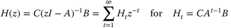
where ![]() is the
is the ![]() unit impulse response matrix with
unit impulse response matrix with ![]() . Here
. Here ![]() is defined as the Markov sequence with the corresponding set of Markov parameters given by the embedded system
is defined as the Markov sequence with the corresponding set of Markov parameters given by the embedded system ![]() .
.
If the MIMO transfer function matrix is available, then the impulse response (matrix) sequence ![]() can be determined simply by long division of each matrix component
can be determined simply by long division of each matrix component ![]() transfer function, that is,
transfer function, that is, ![]() . Consider the following example to illustrate this calculation that will prove useful in the classical realization theory of Chapter 6.
. Consider the following example to illustrate this calculation that will prove useful in the classical realization theory of Chapter 6.
We know from the Cayley–Hamilton theorem of linear algebra that an ![]() ‐dimensional matrix satisfies its own characteristic equation [4]
‐dimensional matrix satisfies its own characteristic equation [4]
Therefore, pre‐ and postmultiplying this relation by the measurement and input transmission matrices ![]() and
and ![]() , respectively, it follows that the Markov parameters satisfy the recursion for the
, respectively, it follows that the Markov parameters satisfy the recursion for the ![]() ‐degree
‐degree ![]()

This result will have critical realizability conditions subsequently in Chapter 6.
The problem of determining the internal description ![]() from the external description (
from the external description (![]() or
or ![]() ) of Eq. 3.32 is called the realization problem. Out of all possible realizations,
) of Eq. 3.32 is called the realization problem. Out of all possible realizations, ![]() having the same Markov parameters, those of smallest dimension are defined as minimal realizations. Thus, the dimension of the minimal realization is identical to the degree of the characteristic polynomial (actually the minimal polynomial for multivariable systems) or equivalently the degree of the transfer function (number of system poles).
having the same Markov parameters, those of smallest dimension are defined as minimal realizations. Thus, the dimension of the minimal realization is identical to the degree of the characteristic polynomial (actually the minimal polynomial for multivariable systems) or equivalently the degree of the transfer function (number of system poles).
In order to develop these relations, we define the ![]() Hankel matrix by
Hankel matrix by
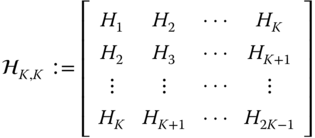
Suppose the dimension of the system is ![]() , then the Hankel matrix could be constructed such that
, then the Hankel matrix could be constructed such that ![]() using
using ![]() impulse response matrices. Knowledge of the order
impulse response matrices. Knowledge of the order ![]() indicates the minimum number of terms required to exactly “match” the Markov sequence and extract the Markov parameters. Also the
indicates the minimum number of terms required to exactly “match” the Markov sequence and extract the Markov parameters. Also the ![]() is the dimension of the minimal realization. If we did not know the dimension of the system, then we would let (in theory)
is the dimension of the minimal realization. If we did not know the dimension of the system, then we would let (in theory) ![]() and determine the rank of
and determine the rank of ![]() . Therefore, the minimal dimension of an “unknown” system is the rank of the Hankel matrix.
. Therefore, the minimal dimension of an “unknown” system is the rank of the Hankel matrix.
In order for a system to be minimal, it must be completely controllable and completely observable [4] . This can be seen from the fact that the Hankel matrix factors as
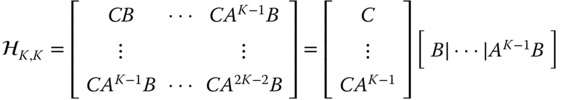
or simply
From this factorization, it follows that the ![]() . Therefore, we see that the properties of controllability and observability are carefully woven into that of minimality and testing the rank of the Hankel matrix yields the dimensionality of the underlying dynamic system. This fact will prove crucial when we “identify” a system,
. Therefore, we see that the properties of controllability and observability are carefully woven into that of minimality and testing the rank of the Hankel matrix yields the dimensionality of the underlying dynamic system. This fact will prove crucial when we “identify” a system, ![]() , from noisy measurement data. We shall discuss realization theory in more detail in Chapter 6 using these results.
, from noisy measurement data. We shall discuss realization theory in more detail in Chapter 6 using these results.
3.4.3 Equivalent Linear Systems
Equivalent systems are based on the concept that there are an infinite number of state‐space systems that possess “identical” input/output responses. In the state‐space, this is termed a set of coordinates; that is, we can change the state vectors describing a system by a similarity transformation such that the system matrices ![]() are transformed to a different set of coordinates by the transformation matrix
are transformed to a different set of coordinates by the transformation matrix ![]() [ 1
–5], that is,
[ 1
–5], that is,
where we have
yields an “equivalent” system from an input/output perspective, that is, the transfer functions are identical

as well as the corresponding impulse response matrices
There does exist unique representations of state‐space systems termed “canonical forms,” which we will see in Section 3.7 for SISO systems as well as for MIMO systems discussed subsequently in Chapter 6. In fact, much of control theory is based on designing controllers in a modal coordinate system with a diagonal system or modal matrix ![]() and then transforming the modal system back to the physical coordinates using the inverse transform
and then transforming the modal system back to the physical coordinates using the inverse transform ![]() [4]
.
[4]
.
3.4.4 Stable Linear Systems
Stability of a linear system can also be cast in conjunction with the properties of controllability and observability [ 4
–10]. For a homogeneous, discrete system, it has been shown that asymptotic stability follows directly from the eigenvalues of the system matrix expressed as ![]() . These eigenvalues must lie within the unit circle or equivalently
. These eigenvalues must lie within the unit circle or equivalently ![]() .
.
Besides determining eigenvalues of ![]() or equivalently factoring the characteristic equation to extract the system poles, another way to evaluate this condition follows directly from Lyapunov stability theory [9, 10
] that incorporates observability.
or equivalently factoring the characteristic equation to extract the system poles, another way to evaluate this condition follows directly from Lyapunov stability theory [9, 10
] that incorporates observability.
An observable system is stable if and only if the Lyapunov equation
has a unique positive definite solution, ![]() . The proof is available in [9]
or [10]
. As we shall see, this is an important property that will appear in subspace identification theory when extracting a so‐called balanced realization as well as a unique stochastic realization [10]
.
. The proof is available in [9]
or [10]
. As we shall see, this is an important property that will appear in subspace identification theory when extracting a so‐called balanced realization as well as a unique stochastic realization [10]
.
This completes the section on discrete systems theory. It should be noted that all of the properties discussed in this section exist for continuous‐time systems as well (see [2] for details).
3.5 Gauss–Markov State‐Space Models
In this section, we extend the state‐space representation to incorporate random inputs or noise sources along with random initial conditions. The discrete‐time Gauss–Markov model will be applied extensively throughout this text.
3.5.1 Discrete‐Time Gauss–Markov Models
Here we investigate the case when random inputs are applied to a discrete state‐space system with random initial conditions. If the excitation is a random signal, then the state is also random. Restricting the input to be deterministic ![]() and the noise to be zero‐mean, white, Gaussian
and the noise to be zero‐mean, white, Gaussian ![]() , the Gauss–Markov model evolves as
, the Gauss–Markov model evolves as
where ![]() and
and ![]()
The solution to the Gauss–Markov equations can easily be obtained by induction to give

which is Markov depending only on the previous state. Since ![]() is just a linear transformation of Gaussian processes, it is also Gaussian. Thus, we can represent a Gauss–Markov process easily employing the state‐space models.
is just a linear transformation of Gaussian processes, it is also Gaussian. Thus, we can represent a Gauss–Markov process easily employing the state‐space models.
When the measurement model is also included, we have
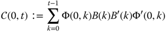
where ![]() . The model is shown diagrammatically in Figure 3.1.
. The model is shown diagrammatically in Figure 3.1.
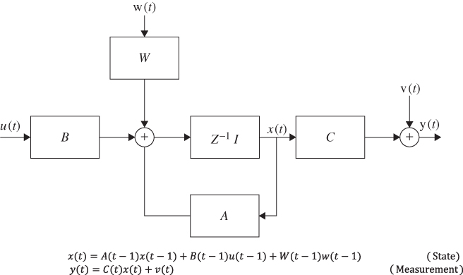
Figure 3.1 Gauss–Markov model of a discrete process.
Since the Gauss–Markov model of Eq. 3.57 is characterized by a Gaussian distribution, it is completely specified (statistically) by its mean and variance. Therefore, if we take the expectation of Eqs. 3.57
and 3.59 respectively, we obtain the state mean vector ![]() as
as
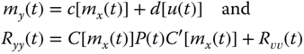
and the measurement mean vector ![]() as
as
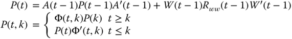
The state variance3 ![]() is given by the discrete Lyapunov equation:
is given by the discrete Lyapunov equation:
and the measurement variance, ![]() is
is
Similarly, it can be shown that the state covariance propagates according to the following equations:

We summarize the Gauss–Markov and corresponding statistical models in Table 3.1.
Table 3.1 Gauss–Markov representation.
| State propagation |
|
|
| State mean propagation |
|
|
| State variance/covariance propagation |
|
| Measurement propagation |
|
|
| Measurement mean propagation |
|
|
| Measurement variance/covariance propagation |

|
If we restrict the Gauss–Markov model to the stationary case, then

and the variance equations become
with
At steady state (![]() ), we have
), we have
and therefore, the measurement covariance relations become
By induction, it can be shown that
The measurement power spectrum is easily obtained by taking the ![]() ‐transform of this equation to obtain
‐transform of this equation to obtain
where
with
Thus, using ![]() the spectrum is given by
the spectrum is given by
So we see that the Gauss–Markov state‐space model enables us to have a more general representation of a multichannel stochastic signal. In fact, we are able to easily handle the multichannel and nonstationary statistical cases within this framework. Generalizations are also possible with the vector models, but those forms become quite complicated and require some knowledge of multivariable systems theory and canonical forms (see [1] for details). Before we leave this subject, let us consider a simple input/output example with Gauss–Markov models.

Figure 3.2 Gauss–Markov simulation of first‐order process: (a) state/measurement means, (b) state with  confidence interval about its mean, and (c) Measurement with
  confidence interval about its mean.
It should be noted that if the bounds are exceeded by more than ![]() (
(![]() lie within), then we must select a new seed and reexecute the simulation until the bound conditions are satisfied signifying a valid Gauss–Markov simulation.
lie within), then we must select a new seed and reexecute the simulation until the bound conditions are satisfied signifying a valid Gauss–Markov simulation.
3.6 Innovations Model
In this section, we briefly develop the innovations model that is related to the Gauss–Markov representation. The significance of this model will be developed throughout the text, but we take the opportunity now to show its relationship to the basic Gauss–Markov representation. We start by extending the original Gauss–Markov representation to the correlated process and measurement noise case and then show how the innovations model is a special case of this structure.
The standard Gauss–Markov model for correlated process and measurement noise is given by

where ![]() and
and
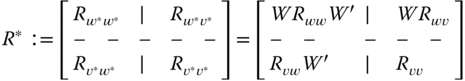
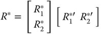
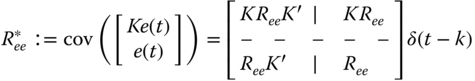
Here we observe that in the standard Gauss–Markov model, the ![]() block covariance matrix,
block covariance matrix, ![]() , is full with cross‐covariance matrices
, is full with cross‐covariance matrices ![]() on its off‐diagonals. The usual standard model assumes that they are null (uncorrelated). To simulate a system with correlated
on its off‐diagonals. The usual standard model assumes that they are null (uncorrelated). To simulate a system with correlated ![]() and
and ![]() is more complicated using this form of the Gauss–Markov model because
is more complicated using this form of the Gauss–Markov model because ![]() must first be factored such that
must first be factored such that
where ![]() are matrix square roots [6,7]. Once the factorization is performed, then the correlated noise is synthesized “coloring” the uncorrelated noise sources,
are matrix square roots [6,7]. Once the factorization is performed, then the correlated noise is synthesized “coloring” the uncorrelated noise sources, ![]() and
and ![]() as
as

The innovations model is a constrained version of the correlated Gauss–Markov characterization. If we assume that ![]() is a zero‐mean, white, Gaussian sequence, that is,
is a zero‐mean, white, Gaussian sequence, that is, ![]() , then the innovations model [11– 15
] evolves as
, then the innovations model [11– 15
] evolves as
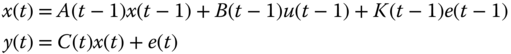
where ![]() is the
is the ![]() ‐dimensional innovations vector and
‐dimensional innovations vector and ![]() is the
is the ![]() weighting matrix with the innovations covariance specified by
weighting matrix with the innovations covariance specified by
It is important to note that the innovations model has implications in Wiener–Kalman filtering (spectral factorization) because ![]() can be represented in factored or square‐root form (
can be represented in factored or square‐root form (![]() ) directly in terms of the weight and innovations covariance matrix as
) directly in terms of the weight and innovations covariance matrix as

Comparing the innovations model to the Gauss–Markov model, we see that they are both equivalent to the case when ![]() and
and ![]() are correlated. Next we show the equivalence of the various model sets to this family of state‐space representations.
are correlated. Next we show the equivalence of the various model sets to this family of state‐space representations.
3.7 State‐Space Model Structures
In this section, we discuss special state‐space structures usually called “canonical forms” in the literature, since they represent unique state constructs that are particularly useful. We will confine the models to SISO forms, while the more complicated multivariable structures will be developed in Chapter 6. Here we will first recall the autoregressive‐moving average model with exogenous inputs ARMAX model of Chapter 2 and then its equivalent representation in the state‐space form.
3.7.1 Time‐Series Models
Time‐series models are particularly useful representations used frequently by statisticians and signal processors to represent time sequences when no physics is available to employ directly. They form the class of black‐box or gray‐box models [15] , which are useful in predicting data. These models have an input/output structure, but they can be transformed to an equivalent state‐space representation. Each model set has its own advantages: the input/output models are easy to use, while the state‐space models are easily generalized and usually evolve when physical phenomenology can be described in a model‐based sense [15] .
We have a difference equation relating the output sequence ![]() to the input sequence
to the input sequence ![]() in terms of the backward shift operator as 4
in terms of the backward shift operator as 4
or
Recall from Section 2.4 that when the system is excited by random inputs, the models can be represented by an ARMAX and is abbreviated by ARMAX(![]() ).
).

where ![]() ,
, ![]() ,
, ![]() , are polynomials in the backward‐shift operator
, are polynomials in the backward‐shift operator ![]() such that
such that ![]() and
and ![]() is a white noise source with coloring filter
is a white noise source with coloring filter
Since the ARMAX model is used to characterize a random signal, we are interested in its statistical properties (see [15] for details). We summarize these properties in Table 3.2.
Table 3.2 ARMAX representation.
| Output propagation | ||
|
|
||
| Mean propagation | ||
|
|
||
| Impulse propagation | ||
|
|
||
| Variance/covariance propagation | ||

|
||
| the output or measurement sequence | ||
| the input sequence | ||
| the process (white) noise sequence with variance |
||
| the impulse response sequence | ||
| the impulse input of amplitude |
||
| the mean output or measurement sequence | ||
| the mean process noise sequence | ||
| the stationary output covariance at lag |
||
| the |
||
| the |
||
| the |
||
This completes the section on ARMAX models.
3.7.2 State‐Space and Time‐Series Equivalence Models
In this section, we show the equivalence between the ARMAX and state‐space models (for scalar processes). That is, we show how to obtain the state‐space model given the ARMAX models by inspection. We choose particular coordinate systems in the state‐space (canonical form) and obtain a relationship between entries of the state‐space system to coefficients of the ARMAX model. An example is presented that shows how these models can be applied to realize a random signal. First, we consider the ARMAX to state‐space transformation.
Recall from Eq. 3.77 that the general difference equation form of the ARMAX model is given by

or equivalently in the frequency domain as

where ![]() and
and ![]() and
and ![]() is a zero‐mean, white sequence with spectrum given by
is a zero‐mean, white sequence with spectrum given by ![]() .
.
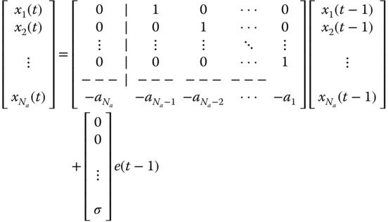
It is straightforward to show (see [5] ) that the ARMAX model can be represented in observer canonical form:

where ![]() and
and ![]() are the
are the ![]() ‐state vector, scalar input, noise, and output with
‐state vector, scalar input, noise, and output with

Noting this structure we see that each of the matrix or vector elements ![]()
![]() can be determined from the relations
can be determined from the relations

where

Consider the following example to illustrate these relations.
It is important to realize that if we assume that ![]() is Gaussian, then the ARMAX model is equivalent to the innovations representation of Section 3.6, that is,
is Gaussian, then the ARMAX model is equivalent to the innovations representation of Section 3.6, that is,

where, in this case, ![]() ,
, ![]() , and
, and ![]() . Also, the corresponding covariance matrix becomes
. Also, the corresponding covariance matrix becomes

This completes the discussion on the equivalence of the general ARMAX to state‐space. Next let us develop the state‐space equivalent models for some of the special cases of the ARMAX model presented in Section 2.4.
We begin with the moving average (MA)
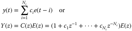
Define the state variable as
and therefore,
Expanding this expression, we obtain

or in vector–matrix form

Thus, the general form for the MA state‐space is given by
with ![]() ,
, ![]() .
.
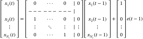
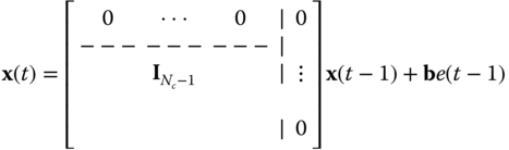
Next consider the autoregressive (AR) model (all‐pole) given by
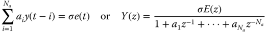
Here the state vector is defined by ![]() and therefore,
and therefore, ![]() with
with ![]() . Expanding over
. Expanding over ![]() , we obtain the vector–matrix state‐space model
, we obtain the vector–matrix state‐space model

In general, we have the AR (all‐pole) state‐space model
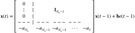
with ![]() ,
, ![]() .
.
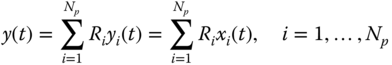
Another useful state‐space representation is the normal form that evolves by performing a partial fraction expansion of a rational discrete transfer function model (ARMA) to obtain

for ![]() the set of residues and poles of
the set of residues and poles of ![]() . Note that the normal form model is the decoupled or parallel system representation based on the following set of relations:
. Note that the normal form model is the decoupled or parallel system representation based on the following set of relations:
Defining the state variable as ![]() , then equivalently
, then equivalently
and therefore, the output is given by
Expanding these relations over ![]() , we obtain
, we obtain


Thus, the general decoupled form of the normal state‐space model is given by
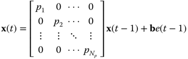
for ![]() with
with ![]() , an
, an ![]() ‐vector of unit elements. Here
‐vector of unit elements. Here ![]() and
and ![]() .
.
3.8 Nonlinear (Approximate) Gauss–Markov State‐Space Models
Many processes in practice are nonlinear, rather than linear. Coupling the nonlinearities with noisy data makes the signal processing problem a challenging one. In this section, we develop an approximate solution to the nonlinear modeling problem involving the linearization of the nonlinear process about a “known” reference trajectory. In this section, we limit our discussion to discrete nonlinear systems. Continuous solutions to this problem are developed in [ 6 – 15 ].
Suppose we model a process by a set of nonlinear stochastic vector difference equations in state‐space form as
with the corresponding measurement model
where ![]() ,
, ![]() ,
, ![]() ,
, ![]() are nonlinear vector functions of
are nonlinear vector functions of ![]() ,
, ![]() , with
, with ![]() ,
, ![]() and
and ![]() ,
, ![]() .
.
Ignoring the additive noise sources, we “linearize” the process and measurement models about a known deterministic reference trajectory defined by ![]() as illustrated in Figure 3.3,5 that is,
as illustrated in Figure 3.3,5 that is,

Figure 3.3 Linearization of a deterministic system using the reference trajectory defined by ( ).
).
Deviations or perturbations from this trajectory are defined by
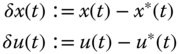
Substituting the previous equations into these expressions, we obtain the perturbation trajectory as
The nonlinear vector functions ![]() and
and ![]() can be expanded into a first‐order Taylor series about the reference trajectory
can be expanded into a first‐order Taylor series about the reference trajectory ![]() as6
as6
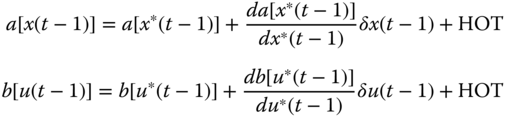
We define the first‐order Jacobian matrices as

Incorporating the definitions of Eq. 3.102 and neglecting the higher order terms (HOT) in Eq. 3.101, the linearized perturbation process model in 3.100 can be expressed as
Similarly, the measurement system can be linearized by using the reference measurement
and applying the Taylor series expansion to the nonlinear measurement model
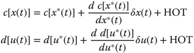
The corresponding measurement perturbation model is defined by
Substituting the first‐order approximations for ![]() and
and ![]() leads to the linearized measurement perturbation as
leads to the linearized measurement perturbation as
where ![]() is defined as the measurement Jacobian.
is defined as the measurement Jacobian.
Summarizing, we have linearized a deterministic nonlinear model using a first‐order Taylor series expansion for the model functions, ![]() ,
, ![]() , and
, and ![]() and then developed a linearized Gauss–Markov perturbation model valid for small deviations from the reference trajectory given by
and then developed a linearized Gauss–Markov perturbation model valid for small deviations from the reference trajectory given by

with ![]() ,
, ![]() ,
, ![]() , and
, and ![]() the corresponding Jacobian matrices with
the corresponding Jacobian matrices with ![]() ,
, ![]() zero‐mean, Gaussian.
zero‐mean, Gaussian.
We can also use linearization techniques to approximate the statistics of the process and measurements. If we use the first‐order Taylor series expansion and expand about the mean, ![]() , rather than
, rather than ![]() , then taking expected values
, then taking expected values
gives
which follows by linearizing ![]() about
about ![]() and taking the expected value.
and taking the expected value.
The variance equations ![]() can also be developed in a similar manner (see [7]
for details) to give
can also be developed in a similar manner (see [7]
for details) to give
Using the same approach, we arrive at the accompanying measurement statistics
We summarize these results in the “approximate” Gauss–Markov model of Table 3.3.
Before we close, consider the following example to illustrate the approximation.
Table 3.3 Approximate nonlinear Gauss–Markov model.
| State propagation |
|
|
| State mean propagation |
|
|
| State covariance propagation |
|
|
| Measurement propagation |
|
|
| Measurement mean propagation |
|
|
| Measurement covariance propagation |
|
|
| Initial conditions |
|
|
| Jacobians |

|
Although the linearization approach discussed here seems somewhat extraneous relative to the previous sections, it becomes a crucial ingredient in the classical approach to (approximate) nonlinear estimation of the subsequent chapters. We discuss the linear state‐space approach (Kalman filter) to the estimation problem in Chapter 4 and then show how these linearization concepts can be used to solve the nonlinear estimation problem. There the popular “extended” Kalman filter processor relies heavily on these linearization techniques developed in this section for its development.
3.9 Summary
In this chapter, we have discussed the development of continuous‐time, sampled‐data, and discrete‐time state‐space models. The stochastic variants of the deterministic models were presented leading to the Gauss–Markov representations for both linear and (approximate) nonlinear systems. The discussion of both the deterministic and stochastic state‐space models included a brief development of their second‐order statistics. We also discussed the underlying discrete systems theory as well as a variety of time‐series models (ARMAX, AR, MA, etc.) and showed that they can easily be represented in state‐space form through the use of canonical forms (models). These models form the embedded structure incorporated into the model‐based processors that will be discussed in subsequent chapters. We concluded the chapter with a brief development of a “linearized” nonlinear model leading to an approximate Gauss–Markov representation.
MATLAB Notes
MATLAB has many commands to convert to/from state‐space models to other forms useful in signal processing. Many of them reside in the Signal Processing and Control Systems toolboxes. The matrix exponential is invoked by the expm command and is determined from Taylor/Padé approximants using the scaling and squaring approach. Also the commands expmdemo1, expmdemo2, and expmdemo3 demonstrate the trade‐offs of the Padé, Taylor, and eigenvector approaches to calculate the matrix exponential. The ordinary differential equation method is available using the wide variety of numerical integrators available (ode*). Converting to/from transfer functions and state‐space is accomplished using the ss2tf and tf2ss commands, respectively. ARMAX simulations are easily accomplished using the filter command with a variety of options converting from ARMAX‐to/from transfer functions. The Identification Toolbox converts polynomial‐based models to state‐space and continuous parameters including Gauss–Markov to discrete parameters (th2ss, thc2thd, thd2thc).
References
- 1 Kailath, T. (1980). Linear Systems. Englewood Cliffs, NJ: Prentice‐Hall.
- 2 Szidarovszky, F. and Bahill, A. (1980). Linear Systems Theory. Boca Raton, FL: CRC Press.
- 3 DeCarlo, R. (1989). Linear Systems: A State Variable Approach. Englewood Cliffs, NJ: Prentice‐Hall.
- 4 Chen, C. (1984). Introduction to Linear System Theory. New York: Holt, Rinehart, and Winston.
- 5 Tretter, S. (1976). Introduction to Discrete‐Time Signal Processing. New York: Wiley.
- 6 Jazwinski, A. (1970). Stochastic Processes and Filtering Theory. New York: Academic Press.
- 7 Sage, A. and Melsa, J. (1971). Estimation Theory with Applications to Communications and Control. New York: McGraw‐Hill.
- 8 Maybeck, P. (1979). Stochastic Models, Estimation and Control, vol. 1. New York: Academic Press.
- 9 Anderson, B. and Moore, J. (2005). Optimal Filtering. Mineola, NY: Dover Publications.
- 10 Katayama, T. (2005). Subspace Methods for System Identification. London: Springer.
- 11 Goodwin, G. and Payne, R.L. (1976). Dynamic System Identification. New York: Academic Press.
- 12 Goodwin, G. and Sin, K. (1984). Adaptive Filtering, Prediction and Control. Englewood Cliffs, NJ: Prentice‐Hall.
- 13 Mendel, J. (1995). Lessons in Estimation Theory for Signal Processing, Communications, and Control. Englewood Cliffs, NJ: Prentice‐Hall.
- 14 Brown, R. and Hwang, P.C. (1997). Introduction to Random Signals and Applied Kalman Filtering. New York: Wiley.
- 15 Candy, J. (2006). Model‐Based Signal Processing. Hoboken, NJ: Wiley/IEEE Press.
- 16 Robinson, E. and Silvia, M. (1979). Digital Foundations of Time Series Analysis, vol. 1. San Francisco, CA: Holden‐Day.
- 17 Simon, D. (2006). Optimal State Estimation Kalman,
 and Nonlinear Approaches. Hoboken, NJ: Wiley.
 - 18 Grewal, M.S. and Andrews, A.P. (1993). Kalman Filtering: Theory and Practice. Englewood Cliffs, NJ: Prentice‐Hall.
- 19 Moler, C. and Van Loan, C. (2003). Nineteen dubious ways to compute the exponential of a matrix, twenty‐five years later. SIAM Rev. 45 (1): 3–49.
- 20 Golub, G. and Van Loan, C. (1989). Matrix Computation. Baltimore, MA: Johns Hopkins University Press.
- 21 Ho, B. and Kalman, R. (1966). Effective reconstruction of linear state variable models from input/output data. Regelungstechnik 14: 545–548.
- 22 Candy, J., Warren, M., and Bullock, T. (1977). Realization of an invariant system description from Markov sequences. IEEE Trans. Autom. Control 23 (7): 93–96.
- 23 Kung, S., Arun, K., and Bhaskar Rao, D. (1983). State‐space and singular‐value decomposition‐based approximation methods for the harmonic retrieval problem. J. Opt. Soc. Am. 73 (12): 1799–1811.
Problems
3.1 Derive the following properties of conditional expectations:
 if
if  and
and  are independent.
 .
. .
. .
. .
. .
. .
.
(Hint: See Appendix A.1.)
- 3.2 Suppose
 ,
,  ,
,  are Gaussian random variables with corresponding means
  ,
,  ,
,  and variances
  ,
,  ,
,  show that:
- If
 ,
,  constants, then
 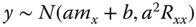 .
. - If
 and
and  are uncorrelated, then they are independent.
 - If
 are Gaussian with mean
  and variance
  , then for

- If
 and
and  are jointly (conditionally) Gaussian, then

- The random variable
 is orthogonal to
  .
. - If
 and
and  are independent, then

- If
 and
and  are not independent, show that
for
are not independent, show that
for
 .
.
(Hint: See Appendices A.1–A.3.)
- If
- 3.3 Suppose we are given the factored power spectrum
 with
with

- Develop the ARMAX model for the process.
- Develop the corresponding Gauss–Markov model for both the standard and innovations representation of the process.
- 3.4 We are given the following Gauss–Markov model
- Calculate the state power spectrum,
 .
. - Calculate the measurement power spectrum,
 .
. - Calculate the state covariance recursion,
 .
. - Calculate the steady‐state covariance,
 .
. - Calculate the output covariance recursion,
 .
. - Calculate the steady‐state output covariance,
 .
.
- Calculate the state power spectrum,
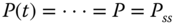
- 3.5 Suppose we are given the Gauss–Markov process characterized by the state equations

for
 a step of amplitude 0.03 and
  and
and  .
.- Calculate the covariance of
 , i.e.
  .
. - Since the process is stationary, we know that
What is the steady‐state covariance,

 , of this process?
 - Develop a MATLAB program to simulate this process.
- Plot the process
 with the corresponding confidence limits
  for 100 data points, do 95% of the samples lie within the bounds?
- Calculate the covariance of
- 3.6 Suppose we are given the ARMAX model
- What is the corresponding innovations model in state‐space form for
 ?
? - Calculate the corresponding covariance matrix
 .
.
- What is the corresponding innovations model in state‐space form for
- 3.7 Given a continuous–discrete Gauss–Markov model

where
 and
and  are zero‐mean and white with respective covariances,
  and
and  , along with a piecewise constant input,
  .
.- Develop the continuous–discrete mean and covariance propagation models for this system.
- Suppose
 is processed by a coloring filter that exponentially correlates it,
  . Develop the continuous–discrete Gauss–Markov model in this case.
- 3.8
Develop the continuous–discrete Gauss–Markov models for the following systems:
- Wiener process:
 ;
;  ,
,  is zero‐mean, white with
  .
. - Random bias:
 ;
;  where
where  .
. - Random ramp:
 ;
;  .
. - Random oscillation:
 ;
;  .
. - Random second order:
 ;
;  .
.
- Wiener process:
- 3.9
Develop the continuous–discrete Gauss–Markov model for correlated process noise, that is,

- 3.10 Develop the approximate Gauss–Markov model for the following nonlinear state transition and measurement model are given by
where
 and
and  . The initial state is Gaussian distributed with
  .
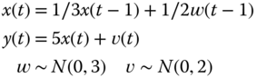
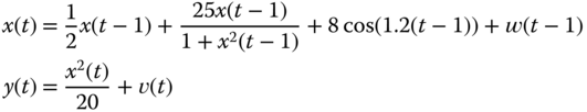
. - 3.11 Consider the discrete nonlinear process given by

with corresponding measurement model
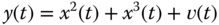
where
 and
and  . The initial state is Gaussian distributed with
  .
.Develop the approximate Gauss–Markov process model for this nonlinear system.