
4
Model‐Based Processors
4.1 Introduction
In this chapter, we introduce the fundamental concepts of model‐based signal processing using state‐space models 1,2. We first develop the paradigm using the linear, (time‐varying) Gauss–Markov model of the previous chapter and then investigate the required conditional expectations leading to the well‐known linear Kalman filter (LKF) processor 3. Based on this fundamental theme, we progress to the idea of the linearization of a nonlinear, state‐space model also discussed in the previous chapter, where we investigate a linearized processor – the linearized Kalman filter (LZKF). It is shown that the resulting processor can provide a solution (time‐varying) to the nonlinear state estimation. We then develop the extended Kalman filter (EKF) as a special case of the LZKF, linearizing about the most available state estimate, rather than a reference trajectory. Next we take it one step further to briefly discuss the iterated–extended Kalman filter (IEKF) demonstrating improved performance.
We introduce an entirely different approach to Kalman filtering – the unscented Kalman filter (UKF) that evolves from a statistical linearization, rather than a dynamic model linearization of the previous suite of nonlinear approaches. The theory is based on the concept of “sigma‐point” transformations that enable a much better matching of first‐ and second‐order statistics of the assumed posterior distribution with even higher orders achievable.
Finally, we return to the basic Bayesian approach of estimating the posterior state distribution directly leading to the particle filter (PF). Here following the Bayesian paradigm, the processor, which incorporates the nonlinear state‐space model, produces a nonparametric estimate of the desired posterior at each time‐step. Computationally more intense, but it is capable of operating in both non‐Gaussian and multimodal distribution environments. From this perspective, it is important to realize that the LKF is essentially an efficient recursive technique that estimates the conditional mean and covariance of the posterior Gaussian distribution, but is incapable of dealing with multimodal, non‐Gaussian problems effectively.
We summarize the results with a case study implementing a 2D‐tracking filter.
4.2 Linear Model‐Based Processor: Kalman Filter
We develop the model‐based processors (MBP) for the dynamic estimation problem, that is, the estimation of state processes that vary with time. Here the state‐space representation is employed as the basic model embedded in the algorithm. To start with, we present the Kalman filter algorithm in the predictor–corrector form. We use this form because it provides insight into the operation of this state‐space (MBP) as well as the other recursive processors to follow.
Table 4.1 Linear Kalman filter algorithm (predictor–corrector form).
| Prediction | |
|
|
(State Prediction) |
|
|
(Measurement Prediction) |
|
|
(Covariance Prediction) |
| Innovations | |
|
|
(Innovations) |
|
|
(Innovations Covariance) |
| Gain | |
|
|
(Gain or Weight) |
| Correction | |
|
|
(State Correction) |
|
|
(Covariance Correction) |
| Initial conditions | |
|
|
|
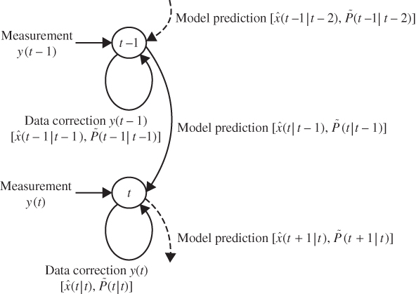
Figure 4.1 Predictor–corrector form of the Kalman filter: Timing diagram.
The operation of the MBP algorithm can be viewed as a predictor–corrector algorithm as in standard numerical integration. Referring to the algorithm in Table 4.1 and Figure 4.1, we see its inherent timing in the algorithm. First, suppose we are currently at time ![]() and have not received a measurement,
and have not received a measurement, ![]() as yet. We have the previous filtered estimate
as yet. We have the previous filtered estimate ![]() and error covariance
and error covariance ![]() and would like to obtain the best estimate of the state based on
and would like to obtain the best estimate of the state based on ![]() data samples. We are in the “prediction phase” of the algorithm. We use the state‐space model to predict the state estimate
data samples. We are in the “prediction phase” of the algorithm. We use the state‐space model to predict the state estimate ![]() and its associated error covariance
and its associated error covariance ![]() . Once the prediction based on the model is completed, we then calculate the innovations covariance
. Once the prediction based on the model is completed, we then calculate the innovations covariance ![]() and gain
and gain ![]() . As soon as the measurement at time
. As soon as the measurement at time ![]() , that is,
, that is, ![]() , becomes available, then we determine the innovations
, becomes available, then we determine the innovations ![]() . Now we enter the “correction phase” of the algorithm. Here we correct or update the state based on the new information in the measurement – the innovations. The old, or predicted, state estimate
. Now we enter the “correction phase” of the algorithm. Here we correct or update the state based on the new information in the measurement – the innovations. The old, or predicted, state estimate ![]() is used to form the filtered, or corrected, state estimate
is used to form the filtered, or corrected, state estimate ![]() and
and ![]() . Here we see that the error, or innovations, is the difference between the actual measurement and the predicted measurement
. Here we see that the error, or innovations, is the difference between the actual measurement and the predicted measurement ![]() . The innovations is weighted by the gain matrix
. The innovations is weighted by the gain matrix ![]() to correct the old state estimate (predicted)
to correct the old state estimate (predicted) ![]() . The associated error covariance is corrected as well. The algorithm then awaits the next measurement at time
. The associated error covariance is corrected as well. The algorithm then awaits the next measurement at time ![]() . Observe that in the absence of a measurement, the state‐space model is used to perform the prediction, since it provides the best estimate of the state.
. Observe that in the absence of a measurement, the state‐space model is used to perform the prediction, since it provides the best estimate of the state.
The covariance equations can be interpreted in terms of the various signal (state) and noise models (see Table 4.1
). The first term of the predicted covariance ![]() relates to the uncertainty in predicting the state using the model
relates to the uncertainty in predicting the state using the model ![]() . The second term indicates the increase in error variance due to the contribution of the process noise
. The second term indicates the increase in error variance due to the contribution of the process noise ![]() or model uncertainty. The corrected covariance equation indicates the predicted error covariance or uncertainty due to the prediction, decreased by the effect of the update (KC), thereby producing the corrected error covariance
or model uncertainty. The corrected covariance equation indicates the predicted error covariance or uncertainty due to the prediction, decreased by the effect of the update (KC), thereby producing the corrected error covariance ![]() . The application of the LKF to the
. The application of the LKF to the ![]() circuit was shown in Figure 1.8, where we see the noisy data, the “true” (mean) output voltage, and the Kalman filter predicted measurement voltage. As illustrated, the filter performs reasonably compared to the noisy data and tracks the true signal quite well. We derive the Kalman filter algorithm from the innovations viewpoint to follow, since it will provide the foundation for the nonlinear algorithms to follow.
circuit was shown in Figure 1.8, where we see the noisy data, the “true” (mean) output voltage, and the Kalman filter predicted measurement voltage. As illustrated, the filter performs reasonably compared to the noisy data and tracks the true signal quite well. We derive the Kalman filter algorithm from the innovations viewpoint to follow, since it will provide the foundation for the nonlinear algorithms to follow.
4.2.1 Innovations Approach
In this section, we briefly develop the (linear) Kalman filter algorithm from the innovations perspective following the approach by Kailath 4–6. First, recall from Chapter 2 that a model of a stochastic process can be characterized by the Gauss–Markov model using the state‐space representation
where ![]() is assumed zero‐mean and white with covariance
is assumed zero‐mean and white with covariance ![]() and
and ![]() and
and ![]() are uncorrelated. The measurement model is given by
are uncorrelated. The measurement model is given by
where ![]() is a zero‐mean, white sequence with covariance
is a zero‐mean, white sequence with covariance ![]() and
and ![]() is (assumed) uncorrelated with
is (assumed) uncorrelated with ![]() and
and ![]() .
.
The linear state estimation problem can be stated in terms of the preceding state‐space model as
GIVEN a set of noisy measurements ![]() , for
, for ![]() characterized by the measurement model of Eq. (4.2), FIND the linear minimum (error) variance estimate of the state characterized by the state‐space model of Eq. (4.1). That is, find the best estimate of
characterized by the measurement model of Eq. (4.2), FIND the linear minimum (error) variance estimate of the state characterized by the state‐space model of Eq. (4.1). That is, find the best estimate of ![]() given the measurement data up to time
given the measurement data up to time ![]() ,
, ![]() .
.
First, we investigate the batch minimum variance estimator for this problem, and then we develop an alternative solution using the innovations sequence. The recursive solution follows almost immediately from the innovations. Next, we outline the resulting equations for the predicted state, gain, and innovations. The corrected, or filtered, state equation then follows. Details of the derivation can be found in 2 .
Constraining the estimator to be linear, we see that for a batch of ![]() ‐data, the minimum variance estimator is given by
1
‐data, the minimum variance estimator is given by
1
where ![]() and
and ![]() , and
, and ![]() . Similarly, the linear estimator can be expressed in terms of the
. Similarly, the linear estimator can be expressed in terms of the ![]() data samples as
data samples as
where ![]() .
.
Here we are investigating a “batch” solution to the state estimation problem, since all the ![]() ‐vector data
‐vector data ![]() are processed in one batch. However, we require a recursive solution (see Chapter 1) to this problem of the form
are processed in one batch. However, we require a recursive solution (see Chapter 1) to this problem of the form
In order to achieve the recursive solution, it is necessary to transform the covariance matrix ![]() to be block diagonal.
to be block diagonal. ![]() block diagonal implies that all the off‐diagonal block matrices
block diagonal implies that all the off‐diagonal block matrices ![]() , for
, for ![]() , which in turn implies that the
, which in turn implies that the ![]() must be uncorrelated or equivalently orthogonal. Therefore, we must construct a sequence of independent
must be uncorrelated or equivalently orthogonal. Therefore, we must construct a sequence of independent ![]() ‐vectors, say
‐vectors, say ![]() , such that
, such that
The sequence ![]() can be constructed using the orthogonality property of the minimum variance estimator such that
can be constructed using the orthogonality property of the minimum variance estimator such that

We define the innovations or new information 4 as
with the orthogonality property that
Since ![]() is a time‐uncorrelated
is a time‐uncorrelated ![]() ‐vector sequence by construction, we have that the block diagonal innovations covariance matrix is
‐vector sequence by construction, we have that the block diagonal innovations covariance matrix is ![]() with each
with each ![]() .
.
The correlated measurement vector can be transformed to an uncorrelated innovations vector through a linear transformation, say ![]() , given by
, given by
where ![]() is a nonsingular transformation matrix and
is a nonsingular transformation matrix and ![]() . Multiplying Eq. (4.8) by its transpose and taking expected values, we obtain
. Multiplying Eq. (4.8) by its transpose and taking expected values, we obtain
Similarly, we obtain
Substituting these results into Eq. (4.4) gives
Since the ![]() are time‐uncorrelated by construction,
are time‐uncorrelated by construction, ![]() is block diagonal. From the orthogonality properties of
is block diagonal. From the orthogonality properties of ![]() ,
, ![]() is lower‐block triangular, that is,
is lower‐block triangular, that is,
where ![]() , and
, and ![]() .
.
The recursive filtered solution now follows easily, if we realize that we want the best estimate of ![]() given
given ![]() ; therefore, any block row can be written (for
; therefore, any block row can be written (for ![]() ) as
) as
If we extract the last (![]() th) term out of the sum (recall from Chapter 1), we obtain
th) term out of the sum (recall from Chapter 1), we obtain

or
where ![]() and
and ![]() .
.
So we see that the recursive solution using the innovations sequence instead of the measurement sequence has reduced the computations to inverting a ![]() matrix
matrix ![]() instead of a
instead of a ![]() matrix,
matrix, ![]() . Before we develop the expression for the filtered estimate of Eq. (4.11), let us investigate the innovations sequence more closely. Recall that the minimum variance estimate of
. Before we develop the expression for the filtered estimate of Eq. (4.11), let us investigate the innovations sequence more closely. Recall that the minimum variance estimate of ![]() is just a linear transformation of the minimum variance estimate of
is just a linear transformation of the minimum variance estimate of ![]() , that is,
, that is,
Thus, the innovations can be decomposed using Eqs. ( 4.2 ) and (4.12) as

for ![]() – the predicted state estimation error. Consider the innovations covariance
– the predicted state estimation error. Consider the innovations covariance ![]() using this equation:
using this equation:
This expression yields the following, since ![]() and
and ![]() are uncorrelated:
are uncorrelated:
The cross‐covariance ![]() is obtained as
is obtained as

Using the definition of the estimation error ![]() , substituting for
, substituting for ![]() and from the orthogonality property of the estimation error for dynamic variables 3
, that is,
and from the orthogonality property of the estimation error for dynamic variables 3
, that is,
we obtain
Thus, we see that the weight or gain matrix is given by
Before we can calculate the corrected state estimate, we require the predicted, or old estimate, that is,
If we employ the state‐space model of Eq. ( 4.1 ), then we have from the linearity properties of the conditional expectation
or
However, from the orthogonality property (whiteness) of ![]() , we have
, we have
which is not surprising, since the best estimate of zero‐mean, white noise is zero (unpredictable). Thus, the prediction is given by
To complete the algorithm, the expressions for the predicted and corrected error covariances must be determined. From the definition of predicted estimation error covariance, we see that ![]() satisfies
satisfies
Since ![]() and
and ![]() are uncorrelated, the predicted error covariance
are uncorrelated, the predicted error covariance ![]() can be determined from this relation 2
to give
can be determined from this relation 2
to give
The corrected error covariance ![]() is calculated using the corrected state estimation error and the corresponding state estimate of Eq. ( 4.11
) as
is calculated using the corrected state estimation error and the corresponding state estimate of Eq. ( 4.11
) as

Using this expression, we can calculate the required error covariance from the orthogonality property, ![]() , and Eq. (4.15) 2
yielding the final expression for the corrected error covariance as
, and Eq. (4.15) 2
yielding the final expression for the corrected error covariance as
This completes the brief derivation of the LKF based on the innovations sequence (see 2 for more details). It is clear to see that the innovations sequence holds the “key” to unlocking the mystery of Kalman filter design. In Section 4.2.3, we investigate the statistical properties of the innovations sequence that will enable us to develop a simple procedure to “tune” the MBP.
4.2.2 Bayesian Approach
The Bayesian approach to Kalman filtering follows in this brief development leading to the maximum a posteriori (MAP) estimate of the state vector under the Gauss–Markov model assumptions (see Chapter 3). Detailed derivations can be found in 2 or 7.
We would like to obtain the MAP estimator for the state estimation problem where the underlying Gauss–Markov model with ![]() ,
, ![]() , and
, and ![]() Gaussian distributed. We know that the corresponding state estimate will also be Gaussian, since it is a linear transformation of Gaussian variables.
Gaussian distributed. We know that the corresponding state estimate will also be Gaussian, since it is a linear transformation of Gaussian variables.
It can be shown using Bayes' rule that the a posteriori probability 2 , 7 can be expressed as

Under the Gauss–Markov model assumptions, we know that each of the conditional distributions can be expressed in terms of the Gaussian distribution as follows:
Substituting these probabilities into Eq. (4.22) and combining all constants into a single constant ![]() , we obtain
, we obtain
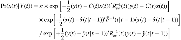
Recognizing the measurement noise, state estimation error, innovations, and taking natural logarithms, we obtain the log a posteriori probability in terms of the Gauss–Markov model as

The MAP estimate is then obtained by differentiating this expression, setting it to zero and solving to obtain

This relation can be simplified by using a form of the matrix inversion lemma 3 , enabling us to eliminate the first bracketed term in Eq. (4.24) to give
Solving for ![]() and substituting gives
and substituting gives

Multiplying out, regrouping terms, and factoring, this relation can be rewritten as

or finally
Further manipulations lead to equivalent expressions for the Kalman gain as
which completes the Bayes' approach to the Kalman filter. A complete detailed derivation is available in 2 or 7 for the interested reader.
4.2.3 Innovations Sequence
In this subsection, we investigate the properties of the innovations sequence, which have been used to develop the Kalman filter 2 . It is interesting to note that since the innovations sequence depends directly on the measurement and is linearly related to it, then it spans the measurement space in which all of our data reside. In contrast, the states or internal variables are not measured directly and are usually not available; therefore, our designs are accomplished using the innovations sequence along with its statistical properties to assure optimality. We call this design procedure minimal (error) variance design.
Recall that the innovations or equivalently the one‐step prediction error is given by
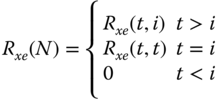
where we define ![]() for
for ![]() – the state estimation error prediction. Using these expressions, we can now analyze the statistical properties of the innovations sequence based on its orthogonality to the measured data. We will state each property first and refer to 2
for proof.
– the state estimation error prediction. Using these expressions, we can now analyze the statistical properties of the innovations sequence based on its orthogonality to the measured data. We will state each property first and refer to 2
for proof.
The innovations sequence is zero‐mean:
The second term is null by definition and the first term is null because ![]() is an unbiased estimator.
is an unbiased estimator.
The innovations sequence is white since
or
The innovations sequence is determined recursively using the Kalman filter and acts as a “Gram–Schmidt orthogonal decomposer” or equivalently whitening filter.
The innovations sequence is also uncorrelated with the deterministic input ![]() since
since
Assuming that the measurement evolves from a Gauss–Markov process as well, then the innovations sequence is merely a linear transformation of Gaussian vectors and is therefore Gaussian with ![]() .
.
Finally, the innovations sequence is related to the measurement by an invertible linear transformation; therefore, it is an equivalent sequence under linear transformations, since either sequence can be constructed from knowledge of the second‐order statistics of the other 2 .
We summarize these properties of the innovations sequence as follows:
- Innovations sequence
 is zero‐mean.
 - Innovations sequence
 is white.
 - Innovations sequence
 is uncorrelated in time and with input
  .
. - Innovations sequence
 is Gaussian with statistics,
  , under the Gauss–Markov assumptions.
 - Innovations
 and measurement
  sequences are equivalent under linear invertible transformations.
The innovations sequence spans the measurement or data space, but in the Kalman filter design problem, we are concerned with the state‐space. Analogous to the innovations sequence in the output space is the predicted state estimation error ![]() in the state‐space. It is easy to show that from the orthogonality condition of the innovations sequence that the corresponding state estimation error is also orthogonal to
in the state‐space. It is easy to show that from the orthogonality condition of the innovations sequence that the corresponding state estimation error is also orthogonal to ![]() , leading to the state orthogonality condition (see 2
for more details).
, leading to the state orthogonality condition (see 2
for more details).
This completes the discussion of the orthogonality properties of the innovations sequence. Next we consider more practical aspects of processor design and how these properties can be exploited to produce a minimum variance processor.
4.2.4 Practical Linear Kalman Filter Design: Performance Analysis
In this section, we heuristically provide an intuitive feel for the operation of the Kalman filter using the state‐space model and Gauss–Markov assumptions. These results coupled with the theoretical points developed in 2 lead to the proper adjustment or “tuning” of the processor. Tuning the processor is considered an art, but with proper statistical tests, the performance can readily be evaluated and adjusted. As mentioned previously, this approach is called the minimum (error) variance design. In contrast to standard filter design procedures in signal processing, the minimum variance design adjusts the statistical parameters (e.g. covariances) of the processor and examines the innovations sequence to determine if the LKF is properly tuned. Once tuned, then all of the statistics (conditional means and variances) are valid and may be used as reasonable estimates. Here we discuss how the parameters can be adjusted and what statistical tests can be performed to evaluate the filter performance.
Heuristically, the Kalman filter can be viewed simply by its update equation:

where ![]() and
and ![]() .
.
Using this representation of the KF, we see that we can view the old or predicted estimate ![]() as a function of the state‐space model
as a function of the state‐space model ![]() and the prediction error or innovations
and the prediction error or innovations ![]() as a function primarily of the new measurement, as indicated in Table 4.1
. Consider the new estimate under the following cases:
as a function primarily of the new measurement, as indicated in Table 4.1
. Consider the new estimate under the following cases:

So we can see that the operation of the processor is pivoted about the values of the gain or weighting matrix ![]() . For small
. For small ![]() , the processor “believes” the model, while for large
, the processor “believes” the model, while for large ![]() , it believes the measurement.
, it believes the measurement.
Let us investigate the gain matrix and see if its variations are consistent with these heuristic notions. First, it was shown in Eq. (4.28) that the alternative form of the gain equation is given by
Thus, the condition where ![]() is small can occur in two cases: (i)
is small can occur in two cases: (i) ![]() is small (fixed
is small (fixed ![]() ), which is consistent because small
), which is consistent because small ![]() implies that the model is adequate; and (ii)
implies that the model is adequate; and (ii) ![]() is large (
is large (![]() fixed), which is also consistent because large
fixed), which is also consistent because large ![]() implies that the measurement is noisy, so again believe the model.
implies that the measurement is noisy, so again believe the model.
For the condition where ![]() is large, two cases can also occur: (i)
is large, two cases can also occur: (i) ![]() is large when
is large when ![]() is large (fixed
is large (fixed ![]() ), implying that the model is inadequate, so believe the measurement; and (ii)
), implying that the model is inadequate, so believe the measurement; and (ii) ![]() is small (
is small (![]() fixed), implying the measurement is good (high signal‐to‐noise ratio [SNR]). So we see that our heuristic notions are based on specific theoretical relationships between the parameters in the KF algorithm of Table 4.2.
fixed), implying the measurement is good (high signal‐to‐noise ratio [SNR]). So we see that our heuristic notions are based on specific theoretical relationships between the parameters in the KF algorithm of Table 4.2.
Table 4.2 Heuristic notions for Kalman filter tuning.
| Kalman filter heuristics | ||
| Condition | Gain | Parameter |
| Believe model | Small |
|
|
|
||
| Believe measurement | Large |
|
|
|
||
Summarizing, a Kalman filter is not functioning properly when the gain becomes small and the measurements still contain information necessary for the estimates. The filter is said to diverge under these conditions. In this case, it is necessary to detect how the filter is functioning and how to adjust it if necessary, but first we consider the tuned LKF.
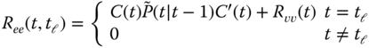
When the processor is “tuned,” it provides an optimal or minimum (error) variance estimate of the state. The innovations sequence, which was instrumental in deriving the processor, also provides the starting point to check the KF operation. A necessary and sufficient condition for a Kalman filter to be optimal is that the innovations sequence is zero‐mean and white (see Ref. 8 for the proof). These are the first properties that must be evaluated to ensure that the processor is operating properly. If we assume that the innovations sequence is ergodic and Gaussian, then we can use the sample mean as the test statistic to estimate, ![]() , the population mean. The sample mean for the
, the population mean. The sample mean for the ![]() th component of
th component of ![]() is given by
is given by
where ![]() and
and ![]() is the number of data samples. We perform a statistical hypothesis test to “decide” if the innovations mean is zero 2
. We test that the mean of the
is the number of data samples. We perform a statistical hypothesis test to “decide” if the innovations mean is zero 2
. We test that the mean of the ![]() th component of the innovations vector
th component of the innovations vector ![]() is
is

As our test statistic, we use the sample mean. At the ![]() ‐significance level, the probability of rejecting the null hypothesis
‐significance level, the probability of rejecting the null hypothesis ![]() is given by
is given by

Therefore, the zero‐mean test 2
on each component innovations ![]() is given by
is given by

Under the null hypothesis ![]() , each
, each ![]() is zero. Therefore, at the 5% significance level (
is zero. Therefore, at the 5% significance level (![]() ), we have that the threshold is
), we have that the threshold is

where ![]() is the sample variance (assuming ergodicity) estimated by
is the sample variance (assuming ergodicity) estimated by
Under the same assumptions, we can perform a whiteness test 2
, that is, check statistically that the innovations covariance corresponds to that of an uncorrelated (white) sequence. Again assuming ergodicity of the innovations sequence, we use the sample covariance function as our test statistic with the ![]() th‐component covariance given by
th‐component covariance given by

We actually use the normalized covariance test statistic

Asymptotically for large ![]() , it can be shown that (see Refs. 2
,9)
, it can be shown that (see Refs. 2
,9)
Therefore, the ![]() confidence interval estimate is
confidence interval estimate is
Hence, under the null hypothesis, ![]() of the
of the ![]() values must lie within this confidence interval, that is, for each component innovations sequence to be considered statistically white. Similar tests can be constructed for the cross‐covariance properties of the innovations 10 as well, that is,
values must lie within this confidence interval, that is, for each component innovations sequence to be considered statistically white. Similar tests can be constructed for the cross‐covariance properties of the innovations 10 as well, that is,
The whiteness test of Eq. (4.38) is very useful for detecting model inaccuracies from individual component innovations. However, for complex systems with a large number of measurement channels, it becomes computationally burdensome to investigate each innovation component‐wise. A statistic capturing all of the innovations information is the weighted sum‐squared residual (WSSR) 9
–11. It aggregates all of the innovations vector information over some finite window of length ![]() . It can be shown that the WSSR is related to a maximum‐likelihood estimate of the normalized innovations variance 2
, 9
. The WSSR test statistic is given by
. It can be shown that the WSSR is related to a maximum‐likelihood estimate of the normalized innovations variance 2
, 9
. The WSSR test statistic is given by
and is based on the hypothesis test

with the WSSR test statistic

Under the null hypothesis, the WSSR is chi‐squared distributed, ![]() . However, for
. However, for ![]() ,
, ![]() is approximately Gaussian
is approximately Gaussian ![]() (see 12 for more details). At the
(see 12 for more details). At the ![]() ‐significance level, the probability of rejecting the null hypothesis is given by
‐significance level, the probability of rejecting the null hypothesis is given by

For a level of significance of ![]() , we have
, we have
Thus, the WSSR can be considered a “whiteness test” of the innovations vector over a finite window of length ![]() . Note that since
. Note that since ![]() are obtained from the state‐space MBP algorithm directly, they can be used for both stationary and nonstationary processes. In fact, in practice, for a large number of measurement components, the WSSR is used to “tune” the filter, and then the component innovations are individually analyzed to detect model mismatches. Also note that the adjustable parameter of the WSSR statistic is the window length
are obtained from the state‐space MBP algorithm directly, they can be used for both stationary and nonstationary processes. In fact, in practice, for a large number of measurement components, the WSSR is used to “tune” the filter, and then the component innovations are individually analyzed to detect model mismatches. Also note that the adjustable parameter of the WSSR statistic is the window length ![]() , which essentially controls the width of the window sliding through the innovations sequence.
, which essentially controls the width of the window sliding through the innovations sequence.
Other sets of “reasonableness” tests can be performed using the covariances estimated by the LKF algorithm and sample variances estimated using Eq. (4.35). The LKF provides estimates of the respective processor covariances ![]() and
and ![]() from the relations given in Table 4.2
. Using sample variance estimators, when the filter reaches steady state, (process is stationary), that is,
from the relations given in Table 4.2
. Using sample variance estimators, when the filter reaches steady state, (process is stationary), that is, ![]() is constant, the estimates can be compared to ensure that they are reasonable. Thus, we have
is constant, the estimates can be compared to ensure that they are reasonable. Thus, we have
Plotting the ![]() and
and ![]() about the component innovations
about the component innovations ![]() and component state estimation errors
and component state estimation errors ![]() , when the true state is known, provides an accurate estimate of the Kalman filter performance especially when simulation is used. If the covariance estimates of the processor are reasonable, then
, when the true state is known, provides an accurate estimate of the Kalman filter performance especially when simulation is used. If the covariance estimates of the processor are reasonable, then ![]() of the sequence samples should lie within the constructed bounds. Violation of these bounds clearly indicates inadequacies in modeling the processor statistics. We summarize these results in Table 4.3 and examine the RC‐circuit design problem in the following example to demonstrate the approach in more detail.
of the sequence samples should lie within the constructed bounds. Violation of these bounds clearly indicates inadequacies in modeling the processor statistics. We summarize these results in Table 4.3 and examine the RC‐circuit design problem in the following example to demonstrate the approach in more detail.
Table 4.3 Statistical tuning tests for Kalman filter.
| Kalman filter design/validation | ||||
| Data | Property | Statistic | Test | Assumptions |
| Innovation |
|
Sample mean | Zero mean | Ergodic, Gaussian |
|
|
Sample covariance | Whiteness | Ergodic, Gaussian | |
|
|
WSSR | Whiteness | Gaussian | |
|
|
Sample cross‐covariance | Cross‐covariance | Ergodic, Gaussian | |
|
|
Sample cross‐covariance | Cross‐covariance | Ergodic, Gaussian | |
| Covariances | Innovation |
Sample variance ( |
|
Ergodic |
| Innovation |
Variance ( |
Confidence interval about |
Ergodic | |
| Estimation error |
Sample variance ( |
|
Ergodic, |
|
| Estimation error |
Variance ( |
Confidence interval about |
|
|
Next we discuss a special case of the KF – a steady‐state Kalman filter that will prove a significant component of the subspace identification algorithms in subsequent chapters.
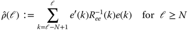
Figure 4.2 LKF design for  ‐circuit problem. (a) Estimated state (voltage) and error. (b) Filtered voltage measurement and error (innovations). (c) WSSR and zero‐mean/whiteness tests.
4.2.5 Steady‐State Kalman Filter
In this section, we discuss a special case of the state‐space LKF – the steady‐state design. Here the data are assumed stationary, leading to a time‐invariant state‐space model, and under certain conditions a constant error covariance and corresponding gain. We first develop the processor and then show how it is precisely equivalent to the classical Wiener filter design. In filtering jargon, this processor is called the steady‐state Kalman filter 13,14.
We briefly develop the steady‐state KF technique in contrast to the usual recursive time‐step algorithms. By steady state, we mean that the processor has embedded time invariant, state‐space model parameters, that is, the underlying model is defined by a set of parameters, ![]() . We state without proof the fundamental theorem (see 3
, 8
, 14
for details).
. We state without proof the fundamental theorem (see 3
, 8
, 14
for details).
If we have a stationary process implying the time‐invariant system, ![]() , and additionally the system is completely controllable and observable and stable (eigenvalues of A lie within the unit circle) with
, and additionally the system is completely controllable and observable and stable (eigenvalues of A lie within the unit circle) with ![]() , then the KF is asymptotically stable. What this means from a pragmatic point of view is that as time increases (to infinity in the limit), the initial error covariance is forgotten as more and more data are processed and that the computation of
, then the KF is asymptotically stable. What this means from a pragmatic point of view is that as time increases (to infinity in the limit), the initial error covariance is forgotten as more and more data are processed and that the computation of ![]() is computationally stable. Furthermore, these conditions imply that
is computationally stable. Furthermore, these conditions imply that
Therefore, this relation implies that we can define a steady‐state gain associated with this covariance as
Let us construct the corresponding steady‐state KF using the correction equation of the state estimator and the steady‐state gain with
therefore, substituting we obtain
but since
we have by substituting into Eq. (4.47) that

with the corresponding steady‐state gain given by
Examining Eq. (4.49) more closely, we see that using the state‐space model, ![]() , and known input sequence,
, and known input sequence, ![]() , we can process the data and extract the corresponding state estimates. The key to the steady‐state KF is calculating
, we can process the data and extract the corresponding state estimates. The key to the steady‐state KF is calculating ![]() , which, in turn, implies that we must calculate the corresponding steady‐state error covariance. This calculation can be accomplished efficiently by combining the prediction and correction relations of Table 4.1
. We have that
, which, in turn, implies that we must calculate the corresponding steady‐state error covariance. This calculation can be accomplished efficiently by combining the prediction and correction relations of Table 4.1
. We have that
which in steady state becomes
There are a variety of efficient methods to calculate the steady‐state error covariance and gain 8
, 14
; however, a brute‐force technique is simply to run the standard predictor–corrector algorithm implemented in UD‐sequential form 15 until the ![]() and therefore
and therefore ![]() converge to constant matrix. Once they converge, it is necessary to only run the algorithm again to process the data using
converge to constant matrix. Once they converge, it is necessary to only run the algorithm again to process the data using ![]() , and the corresponding steady‐state gain will be calculated directly. This is not the most efficient method to solve the problem, but it clearly does not require the development of a new algorithm.
, and the corresponding steady‐state gain will be calculated directly. This is not the most efficient method to solve the problem, but it clearly does not require the development of a new algorithm.
We summarize the steady‐state KF in Table 4.4. We note from the table that the steady‐state covariance/gain calculations depend on the model parameters, ![]() , not the data, implying that they can be precalculated prior to processing the actual data. In fact, the steady‐state processor can be thought of as a simple (multi‐input/multi‐output) digital filter, which is clear if we abuse the notation slightly to write
, not the data, implying that they can be precalculated prior to processing the actual data. In fact, the steady‐state processor can be thought of as a simple (multi‐input/multi‐output) digital filter, which is clear if we abuse the notation slightly to write
For its inherent simplicity compared to the full time‐varying processor, the steady‐state KF is desirable and adequate in many applications, but realize that it will be suboptimal in some cases during the initial transients of the data. However, if we developed the model from first principles, then the underlying physics has been incorporated in the KF, yielding a big advantage over non‐physics‐based designs. This completes the discussion of the steady‐state KF. Next let us reexamine our ![]() ‐circuit problem.
‐circuit problem.
Table 4.4 Steady‐state Kalman filter algorithm.
| Covariance | |
|
|
(steady‐state covariance) |
| Gain | |
|
|
(steady‐state gain) |
| Correction | |
|
|
|
| (state estimate) | |
| Initial Conditions | |
|
|
|
This completes the example. Next we investigate the steady‐state KF and its relation to the Wiener filter.
4.2.6 Kalman Filter/Wiener Filter Equivalence
In this subsection, we show the relationship between the Wiener filter and its state‐space counterpart, the Kalman filter. Detailed proofs of these relations are available for both the continuous and discrete cases 13 . Our approach is to state the Wiener solution and then show that the steady‐state Kalman filter provides a solution with all the necessary properties. We use frequency‐domain techniques to show the equivalence. We choose the frequency domain for historical reasons since the classical Wiener solution has more intuitive appeal. The time‐domain approach will use the batch innovations solution discussed earlier.
The Wiener filter solution in the frequency domain can be solved by spectral factorization 8 since
where ![]() has all its poles and zeros within the unit circle. The classical approach to Wiener filtering can be accomplished in the frequency domain by factoring the power spectral density (PSD) of the measurement sequence; that is,
has all its poles and zeros within the unit circle. The classical approach to Wiener filtering can be accomplished in the frequency domain by factoring the power spectral density (PSD) of the measurement sequence; that is,
The factorization is unique, stable, and minimum phase (see 8 for proof).
Next we show that the steady‐state Kalman filter or the innovations model (ignoring the deterministic input) given by

where ![]() is the zero‐mean, white innovations with covariance
is the zero‐mean, white innovations with covariance ![]() , is stable and minimum phase and, therefore, in fact, the Wiener solution. The “transfer function” of the innovations model is defined as
, is stable and minimum phase and, therefore, in fact, the Wiener solution. The “transfer function” of the innovations model is defined as

and the corresponding measurement PSD is
Using the linear system relations of Chapter 2, we see that
Thus, the measurement PSD is given in terms of the innovations model as
Since ![]() and
and ![]() , then the following (Cholesky) factorization always exists as
, then the following (Cholesky) factorization always exists as
Substituting these factors into Eq. (4.60) gives
Combining like terms enables ![]() to be written in terms of its spectral factors as
to be written in terms of its spectral factors as

or simply
which shows that the innovations model indeed admits a spectral factorization of the type desired. To show that ![]() is the unique, stable, minimum‐phase spectral factor, it is necessary to show that
is the unique, stable, minimum‐phase spectral factor, it is necessary to show that ![]() has all its poles within the unit circle (stable). It has been shown (e.g. 4
, 8
,16) that
has all its poles within the unit circle (stable). It has been shown (e.g. 4
, 8
,16) that ![]() does satisfy these constraints.
does satisfy these constraints.
This completes the discussion on the equivalence of the steady‐state Kalman filter and the Wiener filter. Next we consider the development of nonlinear processors.
4.3 Nonlinear State‐Space Model‐Based Processors
In this section, we develop a suite of recursive, nonlinear state‐space MBPs. We start by using the linearized perturbation model of Section 3.8 and the development of the linear MBP of Section 4.2 to motivate the development of the LZKF. This processor is important in its own right, if a solid reference trajectory is available (e.g. roadmap for a self‐driving vehicle). From this processor, it is possible to easily understand the motivation for the “ad hoc” EKF that follows. Here we see that the reference trajectory is replaced by the most available state estimate. It is interesting to see how the extended filter evolves directly from this relationship. Next we discuss what has become a very popular and robust solution to this nonlinear state estimation problem – the so‐called UKF. Here a statistical linearization replaces the state‐space model linearization approach. Finally, we briefly develop the purely Bayesian approach to solve the nonlinear state estimation problem for both non‐Gaussian and multimodal posterior distribution estimation problems followed by a 2D‐tracking case study completing this chapter.
4.3.1 Nonlinear Model‐Based Processor: Linearized Kalman Filter
In this section, we develop an approximate solution to the nonlinear processing problem involving the linearization of the nonlinear process model about a “known” reference trajectory followed by the development of a MBP based on the underlying linearized state‐space model. Many processes in practice are nonlinear rather than linear. Coupling the nonlinearities with noisy data makes the signal processing problem a challenging one. Here we limit our discussion to discrete nonlinear systems. Continuous‐time solutions to this problem are developed in 3 – 6 , 8 13– 16 .
Recall from Chapter 3 that our process is characterized by a set of nonlinear stochastic vector difference equations in state‐space form as
with the corresponding measurement model
where ![]() ,
, ![]() ,
, ![]() ,
, ![]() are nonlinear vector functions of
are nonlinear vector functions of ![]() ,
, ![]() , and
, and ![]() with
with ![]() ,
, ![]() and
and ![]() ,
, ![]() .
.
In Section 3.8, we linearized a deterministic nonlinear model using a first‐order Taylor series expansion for the functions, ![]() ,
, ![]() , and
, and ![]() and developed a linearized Gauss–Markov perturbation model valid for small deviations given by
and developed a linearized Gauss–Markov perturbation model valid for small deviations given by

with ![]() ,
, ![]() , and
, and ![]() the corresponding Jacobian matrices and
the corresponding Jacobian matrices and ![]() ,
, ![]() zero‐mean, Gaussian.
zero‐mean, Gaussian.
We used linearization techniques to approximate the statistics of Eqs. (4.65) and (4.66) and summarized these results in an “approximate” Gauss–Markov model of Table 3.3. Using this perturbation model, we will now incorporate it to construct a processor that embeds the (![]() ) Jacobian linearized about the reference trajectory [
) Jacobian linearized about the reference trajectory [![]() ]. Each of the Jacobians is deterministic and time‐varying, since they are updated at each time‐step. Replacing the
]. Each of the Jacobians is deterministic and time‐varying, since they are updated at each time‐step. Replacing the ![]() matrices and
matrices and ![]() in Table 4.1
, respectively, by the Jacobians and
in Table 4.1
, respectively, by the Jacobians and ![]() , we obtain the estimated state perturbation
, we obtain the estimated state perturbation
For the Bayesian estimation problem, we are interested in the state estimate ![]() not in its deviation
not in its deviation ![]() . From the definition of the perturbation defined in Section 4.8, we have
. From the definition of the perturbation defined in Section 4.8, we have
where the reference trajectory ![]() was defined as
was defined as
Substituting this relation along with Eq. (4.68) into Eq. (4.69) gives

The corresponding perturbed innovations can also be found directly

where reference measurement ![]() is defined as
is defined as
Using the linear KF with deterministic Jacobian matrices results in
and using this relation and Eq. 4.73 for the reference measurement, we have

Therefore, it follows that the innovations is

The updated estimate is easily found by substituting Eq. ( 4.69 ) to obtain

which yields the identical update equation of Table 4.1
. Since the state perturbation estimation error is identical to the state estimation error, the corresponding error covariance is given by ![]() and, therefore,
and, therefore,
The gain is just a function of the measurement linearization, ![]() completing the algorithm. We summarize the discrete LZKF in Table 4.5.
completing the algorithm. We summarize the discrete LZKF in Table 4.5.
Table 4.5 Linearized Kalman filter (LZKF) algorithm.
| Prediction | |
|
|
|
|
|
|
| (State Prediction) | |
|
|
|
| (Covariance Prediction) | |
| Innovation | |
|
|
|
| (Innovations) | |
|
|
(Innovations Covariance) |
| Gain | |
|
|
(Gain or Weight) |
| Update | |
|
|
(State Update) |
|
|
(Covariance Update) |
| Initial conditions | |
|
|
|
| Jacobians | |
 |
|
 |
|
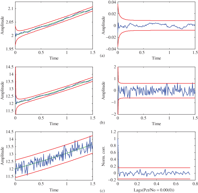
Figure 4.3 Nonlinear trajectory estimation: linearized Kalman filter (LZKF). (a) Estimated state ( out) and error (
 out). (b) Filtered measurement (
 out) and error (innovations) (
 out). (c) Simulated measurement and zero‐mean/whiteness test (
 and
and  out.
out.
4.3.2 Nonlinear Model‐Based Processor: Extended Kalman Filter
In this section, we develop the EKF. The EKF is ad hoc in nature, but has become one of the workhorses of (approximate) nonlinear filtering 3
– 6
, 8
13
–17 more recently being replaced by the UKF 18. It has found applicability in a wide variety of applications such as tracking 19, navigation 3
, 13
, chemical processing 20, ocean acoustics 21, seismology 22 (for further applications see 23). The EKF evolves directly from the linearized processor of Section 4.3.1 in which the reference state, ![]() , used in the linearization process is replaced with the most recently available state estimate,
, used in the linearization process is replaced with the most recently available state estimate, ![]() – this is the step that makes the processor ad hoc. However, we must realize that the Jacobians used in the linearization process are deterministic (but time‐varying) when a reference or perturbation trajectory is used. However, using the current state estimate is an approximation to the conditional mean, which is random, making these associated Jacobians and subsequent relations random. Therefore, although popularly ignored, most EKF designs should be based on ensemble operations to obtain reasonable estimates of the underlying statistics.
– this is the step that makes the processor ad hoc. However, we must realize that the Jacobians used in the linearization process are deterministic (but time‐varying) when a reference or perturbation trajectory is used. However, using the current state estimate is an approximation to the conditional mean, which is random, making these associated Jacobians and subsequent relations random. Therefore, although popularly ignored, most EKF designs should be based on ensemble operations to obtain reasonable estimates of the underlying statistics.
With this in mind, we develop the processor directly from the LZKF. If, instead of using the reference trajectory, we choose to linearize about each new state estimate as soon as it becomes available, then the EKF algorithm results. The reason for choosing to linearize about this estimate is that it represents the best information we have about the state and therefore most likely results in a better reference trajectory (state estimate). As a consequence, large initial estimation errors do not propagate; therefore, linearity assumptions are less likely to be violated. Thus, if we choose to use the current estimate ![]() , where
, where ![]() is
is ![]() or
or ![]() , to linearize about instead of the reference trajectory
, to linearize about instead of the reference trajectory ![]() , then the EKF evolves. That is, let
, then the EKF evolves. That is, let
Then, for instance, when ![]() , the predicted perturbation is
, the predicted perturbation is
Thus, it follows immediately that when ![]() , then
, then ![]() as well.
as well.
Substituting the current estimate, either prediction or update into the LZKF algorithm, it is easy to see that each of the difference terms ![]() is null, resulting in the EKF algorithm. That is, examining the prediction phase of the linearized algorithm, substituting the current available updated estimate,
is null, resulting in the EKF algorithm. That is, examining the prediction phase of the linearized algorithm, substituting the current available updated estimate, ![]() , for the reference and using the fact that (
, for the reference and using the fact that (![]() ), we have
), we have

yielding the prediction of the EKF
Now with the predicted estimate available, substituting it for the reference in Eq. (4.76) gives the innovations sequence as

where we have the new predicted or filtered measurement expression
The updated state estimate is easily obtained by substituting the predicted estimate for the reference (![]() ) in Eq. (4.77)
) in Eq. (4.77)

The covariance and gain equations are identical to those in Table 4.5
, but with the Jacobian matrices ![]() ,
, ![]() ,
, ![]() , and
, and ![]() linearized about the predicted state estimate,
linearized about the predicted state estimate, ![]() . Thus, we obtain the discrete EKF algorithm summarized in Table 4.6. Note that the covariance matrices,
. Thus, we obtain the discrete EKF algorithm summarized in Table 4.6. Note that the covariance matrices, ![]() , and the gain,
, and the gain, ![]() , are now functions of the current state estimate, which is the approximate conditional mean estimate and therefore is a single realization of a stochastic process. Thus, ensemble Monte Carlo
(MC) techniques should be used to evaluate estimator performance. That is, for new initial conditions selected by a Gaussian random number generator (either
, are now functions of the current state estimate, which is the approximate conditional mean estimate and therefore is a single realization of a stochastic process. Thus, ensemble Monte Carlo
(MC) techniques should be used to evaluate estimator performance. That is, for new initial conditions selected by a Gaussian random number generator (either ![]() or
or ![]() ), the algorithm is executed generating a set of estimates, which should be averaged over the entire ensemble using this approach to get an “expected” state, etc. Note also in practice that this algorithm is usually implemented using sequential processing and UD (upper diagonal/square root) factorization techniques (see 15
for details).
), the algorithm is executed generating a set of estimates, which should be averaged over the entire ensemble using this approach to get an “expected” state, etc. Note also in practice that this algorithm is usually implemented using sequential processing and UD (upper diagonal/square root) factorization techniques (see 15
for details).
Table 4.6 Extended Kalman filter (EKF) algorithm.
| Prediction | |
|
|
(State Prediction) |
|
|
|
| (Covariance Prediction) | |
| Innovation | |
|
|
(Innovations) |
|
|
(Innovations Covariance) |
| Gain | |
|
|
(Gain or Weight) |
| Update | |
|
|
(State Update) |
|
|
(Covariance Update) |
| Initial conditions | |
|
|
|
| Jacobians | |
|
|
|
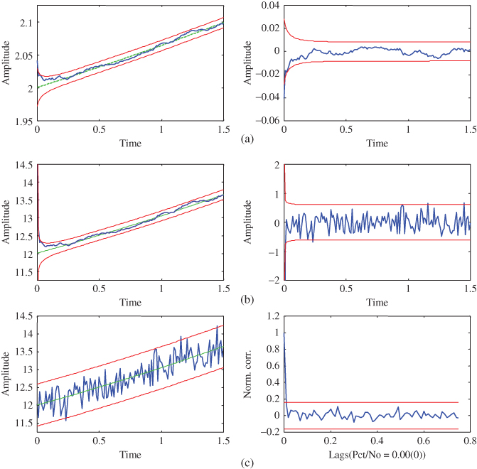
Figure 4.4 Nonlinear trajectory estimation: extended Kalman filter (EKF). (a) Estimated state ( out) and error (
 out). (b) Filtered measurement (
 out) and error (innovations) (
 out). (c) Simulated measurement and zero‐mean/whiteness test (
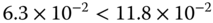 and
and  out).
out).
4.3.3 Nonlinear Model‐Based Processor: Iterated–Extended Kalman Filter
In this section, we discuss an extension of the EKF to the IEKF. This development from the Bayesian perspective coupled to numerical optimization is complex and can be found in 2
. Here we first heuristically motivate the technique and then apply it. This algorithm is based on performing “local” iterations (not global) at a point in time, ![]() to improve the reference trajectory and therefore the underlying estimate in the presence of significant measurement nonlinearities 3
. A local iteration implies that the inherent recursive structure of the processor is retained providing updated estimates as the new measurements are made available.
to improve the reference trajectory and therefore the underlying estimate in the presence of significant measurement nonlinearities 3
. A local iteration implies that the inherent recursive structure of the processor is retained providing updated estimates as the new measurements are made available.
To develop the iterated–extended processor, we start with the linearized processor update relation substituting the “linearized” innovations of Eq. ( 4.76 ) of the LZKF, that is,

where we have explicitly shown the dependence of the gain on the reference trajectory, ![]() through the measurement Jacobian. The EKF algorithm linearizes about the most currently available estimate,
through the measurement Jacobian. The EKF algorithm linearizes about the most currently available estimate, ![]() and
and ![]() in this case. Theoretically, the updated estimate,
in this case. Theoretically, the updated estimate, ![]() , is a better estimate and closer to the true trajectory. Suppose we continue and relinearize about
, is a better estimate and closer to the true trajectory. Suppose we continue and relinearize about ![]() when it becomes available and then recompute the corrected estimate and so on. That is, define the
when it becomes available and then recompute the corrected estimate and so on. That is, define the ![]() th iterated estimate as
th iterated estimate as ![]() , then the corrected or updated iterator equation becomes
, then the corrected or updated iterator equation becomes

Now if we start with the 0th iterate as the predicted estimate, that is, ![]() , then the EKF results for
, then the EKF results for ![]() . Clearly, the corrected estimate in this iteration is given by
. Clearly, the corrected estimate in this iteration is given by
where the last term in this expression is null leaving the usual innovations. Also note that the gain is reevaluated on each iteration as are the measurement function and Jacobian. The iterations continue until there is little difference in consecutive iterates. The last iterate is taken as the updated estimate. The complete (updated) iterative loop is given by

A typical stopping rule is
The IEKF algorithm is summarized in Table 4.7. It is useful in reducing the measurement function nonlinearity approximation errors, improving processor performance. It is designed for measurement nonlinearities and does not improve the previous reference trajectory, but it will improve the subsequent one.
Table 4.7 Iterated–extended Kalman filter (IEKF) algorithm.
| Prediction | |
|
|
(State Prediction) |
|
|
|
| (Covariance Prediction) | |
|
LOOP: |
|
| Innovation | |
|
|
(Innovations) |
|
|
(Innovations Covariance) |
| Gain | |
|
|
(Gain or Weight) |
| Update | |
|
|
(State Update) |
|
|
(Covariance Update) |
| Initial conditions | |
|
|
|
| Jacobians | |
|
|
|
| Stopping rule | |
|
|
|
Figure 4.5 Nonlinear trajectory estimation: Iterated–extended Kalman filter (IEKF). (a) Estimated state ( out) and error (
 out). (b) Filtered measurement (
 out) and error (innovations) (
 out). (c) Simulated measurement and zero‐mean/whiteness test (
 and
and  out).
out).
Next we consider a different approach to nonlinear estimation.
4.3.4 Nonlinear Model‐Based Processor: Unscented Kalman Filter
In this section, we discuss an extension of the approximate nonlinear Kalman filter suite of processors that takes a distinctly different approach to the nonlinear Gaussian problem. Instead of attempting to improve on the linearized model approximation in the nonlinear EKF scheme discussed in Section 4.3.1 or increasing the order of the Taylor series approximations 16 , a statistical transformation approach is developed. It is founded on the basic idea that “it is easier to approximate a probability distribution, than to approximate an arbitrary nonlinear transformation function” 18 ,24,25. The nonlinear processors discussed so far are based on linearizing nonlinear (model) functions of the state and input to provide estimates of the underlying statistics (using Jacobians), while the transformation approach is based upon selecting a set of sample points that capture certain properties of the underlying probability distribution. This set of samples is then nonlinearly transformed or propagated to a new space. The statistics of the new samples are then calculated to provide the required estimates. Once this transformation is performed, the resulting processor, the UKF evolves. The UKF is a recursive processor that resolves some of the approximation issues 24 and deficiencies of the EKF of the previous sections. In fact, it has been called “unscented” because the “EKF stinks.” We first develop the idea of nonlinearly transforming the probability distribution. Then apply it to our Gaussian problem, leading to the UKF algorithm. We apply the processor to the previous nonlinear state estimation problem and investigate its performance.
The unscented transformation (UT) is a technique for calculating the statistics of a random variable that has been transformed, establishing the foundation of the processor. A set of samples or sigma‐points are chosen so that they capture the specific properties of the underlying distribution. Each of the ![]() ‐points is nonlinearly transformed to create a set of samples in the new space. The statistics of the transformed samples are then calculated to provide the desired estimates.
‐points is nonlinearly transformed to create a set of samples in the new space. The statistics of the transformed samples are then calculated to provide the desired estimates.
Consider propagating an ![]() ‐dimensional random vector,
‐dimensional random vector, ![]() , through an arbitrary nonlinear transformation
, through an arbitrary nonlinear transformation ![]() to generate a new random vector 24
to generate a new random vector 24
The set of ![]() ‐points,
‐points, ![]() , consists of
, consists of ![]() vectors with appropriate weights,
vectors with appropriate weights, ![]() , given by
, given by ![]() . The weights can be positive or negative, but must satisfy the normalization constraint that
. The weights can be positive or negative, but must satisfy the normalization constraint that

The problem then becomes
GIVEN these ![]() ‐points and the nonlinear transformation
‐points and the nonlinear transformation ![]() , FIND the statistics of the transformed samples,
, FIND the statistics of the transformed samples, ![]()
The UT approach is to
- Nonlinearly transform each point to obtain the set of new
 ‐points:
- Estimate the posterior mean by its weighted average:

- Estimate the posterior covariance by its weighted outer product:
The critical issues to decide are as follows: (i) ![]() , the number of
, the number of ![]() ‐points; (ii)
‐points; (ii) ![]() , the weights assigned to each
, the weights assigned to each ![]() ‐point; and (iii) where the
‐point; and (iii) where the ![]() ‐points are to be located. The
‐points are to be located. The ![]() ‐points should be selected to capture the “most important” properties of the random vector,
‐points should be selected to capture the “most important” properties of the random vector, ![]() . This parameterization captures the mean and covariance information and permits the direct propagation of this information through the arbitrary set of nonlinear functions. Here we accomplish this (approximately) by generating the discrete distribution having the same first and second (and potentially higher) moments where each point is directly transformed. The mean and covariance of the transformed ensemble can then be computed as the estimate of the nonlinear transformation of the original distribution (see 7
for more details).
. This parameterization captures the mean and covariance information and permits the direct propagation of this information through the arbitrary set of nonlinear functions. Here we accomplish this (approximately) by generating the discrete distribution having the same first and second (and potentially higher) moments where each point is directly transformed. The mean and covariance of the transformed ensemble can then be computed as the estimate of the nonlinear transformation of the original distribution (see 7
for more details).
The UKF is a recursive processor developed to eliminate some of the deficiencies (see 7
for more details) created by the failure of the linearization process to first‐order (Taylor series) in solving the state estimation problem. Different from the EKF, the UKF does not approximate the nonlinear process and measurement models, it employs the true nonlinear models and approximates the underlying Gaussian distribution function of the state variable using the UT of the ![]() ‐points. In the UKF, the state is still represented as Gaussian, but it is specified using the minimal set of deterministically selected samples or
‐points. In the UKF, the state is still represented as Gaussian, but it is specified using the minimal set of deterministically selected samples or ![]() ‐points. These points completely capture the true mean and covariance of the Gaussian distribution. When they are propagated through the true nonlinear process, the posterior mean and covariance are accurately captured to the second order for any nonlinearity with errors only introduced in the third‐order and higher order moments as above.
‐points. These points completely capture the true mean and covariance of the Gaussian distribution. When they are propagated through the true nonlinear process, the posterior mean and covariance are accurately captured to the second order for any nonlinearity with errors only introduced in the third‐order and higher order moments as above.
Suppose we are given an ![]() ‐dimensional Gaussian distribution having covariance,
‐dimensional Gaussian distribution having covariance, ![]() , then we can generate a set of
, then we can generate a set of ![]() ‐points having the same sample covariance from the columns (or rows) of the matrices
‐points having the same sample covariance from the columns (or rows) of the matrices ![]() . Here
. Here ![]() is a scaling factor. This set is zero‐mean, but if the original distribution has mean
is a scaling factor. This set is zero‐mean, but if the original distribution has mean ![]() , then simply adding
, then simply adding ![]() to each of the
to each of the ![]() ‐points yields a symmetric set of
‐points yields a symmetric set of ![]() samples having the desired mean and covariance. Since the set is symmetric, its odd central moments are null, so its first three moments are identical to those of the original Gaussian distribution. This is the minimal number of
samples having the desired mean and covariance. Since the set is symmetric, its odd central moments are null, so its first three moments are identical to those of the original Gaussian distribution. This is the minimal number of ![]() ‐points capable of capturing the essential statistical information. The basic UT technique for a multivariate Gaussian distribution 24
is
‐points capable of capturing the essential statistical information. The basic UT technique for a multivariate Gaussian distribution 24
is
- Compute the set of

 ‐points from the rows or columns of
  . Compute
  .
where
.
where
 is a scalar,
  is the
  th row or column of the matrix square root of
  and
and  is the weight associated with the
  th
th  ‐point.
 - Nonlinearly transform each point to obtain the set of
 ‐points:
  .
. - Estimate the posterior mean of the new samples by its weighted average
- Estimate the posterior covariance of the new samples by its weighted outer product

The discrete nonlinear process model is given by
with the corresponding measurement model
for ![]() and
and ![]() . The critical conditional Gaussian distribution for the state variable statistics is the prior 7
. The critical conditional Gaussian distribution for the state variable statistics is the prior 7
and with the eventual measurement statistics specified by
where ![]() and
and ![]() are the respective corrected state and error covariance based on the data up to time
are the respective corrected state and error covariance based on the data up to time ![]() and
and ![]() ,
, ![]() are the predicted measurement and residual covariance. The idea then is to use the “prior” statistics and perform the UT (under Gaussian assumptions) using both the process and nonlinear transformations (models) as specified above to obtain a set of transformed
are the predicted measurement and residual covariance. The idea then is to use the “prior” statistics and perform the UT (under Gaussian assumptions) using both the process and nonlinear transformations (models) as specified above to obtain a set of transformed ![]() ‐points. Then, the selected
‐points. Then, the selected ![]() ‐points for the Gaussian are transformed using the process and measurement models yielding the corresponding set of
‐points for the Gaussian are transformed using the process and measurement models yielding the corresponding set of ![]() ‐points in the new space. The predicted means are weighted sums of the transformed
‐points in the new space. The predicted means are weighted sums of the transformed ![]() ‐points and covariances are merely weighted sums of their mean‐corrected, outer products.
‐points and covariances are merely weighted sums of their mean‐corrected, outer products.
To develop the UKF we must:
- PREDICT the next state and error covariance,
 , by UT transforming the prior,
  , including the process noise using the
  ‐points
  and
and 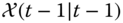 .
. - PREDICT the measurement and residual covariance,
 by using the UT transformed
  ‐points
  and performing the weighted sums.
 - PREDICT the cross‐covariance,
 in order to calculate the corresponding gain for the subsequent correction step.
We use these steps as our road map to develop the UKF. The ![]() ‐points for the UT transformation of the “prior” state information is specified with
‐points for the UT transformation of the “prior” state information is specified with ![]() and
and ![]() ; therefore, we have the UKF algorithm given by
; therefore, we have the UKF algorithm given by
- Select the
 ‐points as:
- Transform (UT) process model:

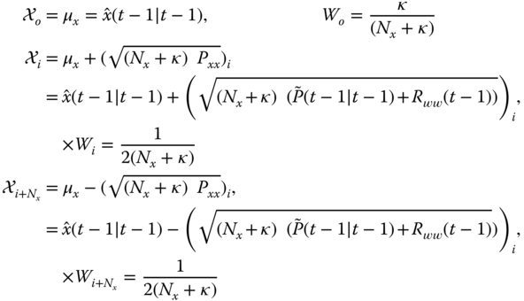
- Estimate the posterior predicted (state) mean by:
- Estimate the posterior predicted (state) residual and error covariance by:

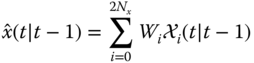
- Transform (UT) measurement (model) with augmented
 ‐points to account for process noise as:
- Estimate the predicted measurement as:
- Estimate the predicted residual and covariance as:

- Estimate the predicted cross‐covariance as:

Clearly with these vectors and matrices available the corresponding gain and update equations follow immediately as
We note that there are no Jacobians calculated and the nonlinear models are employed directly to transform the ![]() ‐points to the new space. Also in the original problem definition, both process and noise sources
‐points to the new space. Also in the original problem definition, both process and noise sources ![]() were assumed additive, but not necessary. For more details of the general process, see the following Refs. 26–28. We summarize the UKF algorithm in Table 4.8.
were assumed additive, but not necessary. For more details of the general process, see the following Refs. 26–28. We summarize the UKF algorithm in Table 4.8.
Table 4.8 Discrete unscented Kalman filter (UKF) algorithm.
| State: σ‐points and weights |
|
|
|
|
|
|
| State prediction |
|
|
|
|
| State error prediction |
|
|
| Measurement: |
| Measurement prediction |
|
|
| Residual prediction |
|
|
|
|
| Gain |
|
|
|
|
| State update |
|
|
|
|
| Initial conditions |
|
|
Before we conclude this discussion, let us apply the UKF to the nonlinear trajectory estimation problem and compare its performance to the other nonlinear processors discussed previously.
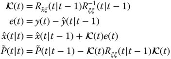
Figure 4.6 Nonlinear trajectory estimation: unscented Kalman filter (UKF). (a) Trajectory (state) estimates using the EKF (thick dotted), IEKF (thin dotted), and UKF (thick solid). (b) Filtered measurement estimates using the EKF (thick dotted), IEKF (thin dotted), and UKF (thick solid). (c) Zero‐mean/whiteness tests for EKF: ( out). (d) Zero‐mean/whiteness tests for IEKF: (
 out). (e) Zero‐mean/whiteness tests for UKF: (
 out).
out).
4.3.5 Practical Nonlinear Model‐Based Processor Design: Performance Analysis
The suite of nonlinear processor designs was primarily developed based on Gaussian assumptions. In the linear Kalman filter case, a necessary and sufficient condition for optimality of the filter is that the corresponding innovations or residual sequence must be zero‐mean and white (see Section 4.2 for details). In lieu of this constraint, a variety of statistical tests (whiteness, uncorrelated inputs, etc.) were developed evolving from this known property. When the linear Kalman filter was “extended” to the nonlinear case, the same tests can be performed based on approximate Gaussian assumptions. Clearly, when noise is additive Gaussian, these arguments can still be applied for improved design and performance evaluation.
In what might be termed “sanity testing,” the classical nonlinear methods employ the basic statistical philosophy that ”if all of the signal information has been removed (explained) from the measurement data, then the residuals (i.e. innovations or prediction error) should be uncorrelated”; that is, the model fits the data and all that remains is a white or uncorrelated residual (innovations) sequence. Therefore, the zero‐mean, whiteness testing, that is, the confidence interval about the normalized correlations (innovations) and the (vector) WSSR tests of Section 4.2 are performed.
Perhaps one of the most important aspects of nonlinear processor design is to recall that processing results only in a single realization of its possible output. For instance, the conditional mean is just a statistic, but still a random process; therefore, if direct measurements are not available, it is best to generate an ensemble of realizations and extract the resulting ensemble statistics using a variety of methods (e.g. bootstrapping 29). In any case, simple ensemble statistics can be employed to provide an average solution enabling us to generate “what we would expect to observe” when the processor is applied to the actual problem. This approach is viable even for the modern nonlinear unscented Kalman processors. Once tuned, the processor is then applied to the raw measurement data, and ensemble statistics are estimated to provide a thorough analysis of the processor performance.
Statistics can be calculated over the ensemble of processor runs. The updated state estimate is obtained directly from the ensemble, that is,
and therefore, the updated state ensemble estimate is
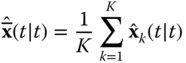
The corresponding predicted state estimate can be obtained directly from the ensemble as well, that is,
and, therefore, the predicted state ensemble estimate is
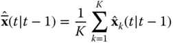
The predicted measurement estimate is also obtained directly from the ensemble, that is,
where recall
Thus, the predicted measurement ensemble estimate is
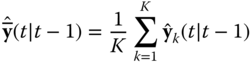
Finally, the corresponding predicted innovations ensemble estimate is given by
and, therefore, the predicted innovations ensemble estimate is
The ensemble residual or innovations sequence can be “sanity tested” for zero‐mean, whiteness, and the mean‐squared error (MSE) over the ensemble to ensure that the processor has been tuned properly. So we see that the ensemble statistics can be estimated and provide a better glimpse of the potential performance of the nonlinear processors for an actual problem. Note that the nonlinear processor examples have applied these ensemble estimates to provide the performance metrics discussed throughout.
4.3.6 Nonlinear Model‐Based Processor: Particle Filter
In this section, we discuss particle‐based processors using the state‐space representation of signals and show how they evolve from the Bayesian perspective using their inherent Markovian structure along with importance sampling techniques as their basic construct. PFs offer an alternative to the Kalman MBPs discussed previously possessing the capability to not just characterize unimodal distributions but also to characterize multimodal distributions. That is, the Kalman estimation techniques suffer from two major shortcomings. First, they are based on linearizations of either the underlying dynamic nonlinear state‐space model (LZKF, EKF, IEKF) or a linearization of a statistical transform (UKF), and, secondly, they are limited to unimodal probability distributions (e.g. Gaussian, Chi‐squared). A PF is a completely different approach to nonlinear estimation that is capable of characterizing multimodal distributions and is not limited by any linearizations. It offers an alternative to approximate Kalman filtering for nonlinear problems 2
,30. In fact, it might be easier to think of the PF as a histogram or kernel density‐like estimator 7
in the sense that it generates an estimated empirical probability mass function (PMF) that approximates the desired posterior distribution such that inferences can be performed and statistics extracted directly. Here the idea is a change in thinking where we attempt to develop a nonparametric empirical estimation of the posterior distribution following a purely Bayesian approach using MC sampling theory as its enabling foundation 7
. As one might expect, the computational burden of the PF is much higher than that of other processors, since it must provide an estimate of the underlying state posterior distribution state‐by‐state at each time‐step along with the fact that the number of random samples to characterize the distribution is equal to the number of particles (![]() ) per time‐step.
) per time‐step.
The PF is a processor that has data on input and produces an estimate of the corresponding posterior distribution on output. These unequally spaced random samples or particles are actually the “location” parameters along with their associated weights that gather or coalesce in the regions of highest probabilities (mean, mode, etc.) providing a nonparametric estimate of the empirical posterior distribution as illustrated in Figure 4.7. With these particles generated, the appropriate weights based on Bayes' rule are estimated from the data and lead to the desired result. Once the posterior is estimated, then inferences can be performed to extract a wealth of descriptive statistics characterizing the underlying process. In particle filtering, continuous distributions are approximated by “discrete” random measures composed of these weighted particles or point masses where the particles are actually random samples of the unknown or hidden states from the state‐space representation and the weights are the approximate “probability masses” estimated recursively. Here in the figure, we see that associated with each particle, ![]() is a corresponding weight or probability mass,
is a corresponding weight or probability mass, ![]() (filled circle). Knowledge of this random measure,
(filled circle). Knowledge of this random measure, ![]() , characterizes an estimate of the instantaneous (at each time
, characterizes an estimate of the instantaneous (at each time ![]() ) filtering posterior distribution (dashed line). The estimated empirical posterior distribution is a weighted PMF given by
) filtering posterior distribution (dashed line). The estimated empirical posterior distribution is a weighted PMF given by


Figure 4.7 Particle filter representation of “empirical” posterior probability distribution in terms of weights (probabilities) and particles (samples).
Thus, the PF does not involve linearizations around current estimates, but rather approximations of the desired distributions by these discrete random measures in contrast to the Kalman filter that sequentially estimates the conditional mean and covariance used to characterize the “known” (Gaussian) filtering posterior, ![]() . PFs are a sequential MC methodology based on this “point mass” representation of probability distributions that only requires a state‐space representation of the underlying process. This representation provides a set of particles that evolve at each time‐step leading to an instantaneous approximation of the target posterior distribution of the state at time
. PFs are a sequential MC methodology based on this “point mass” representation of probability distributions that only requires a state‐space representation of the underlying process. This representation provides a set of particles that evolve at each time‐step leading to an instantaneous approximation of the target posterior distribution of the state at time ![]() given all of the data up to that time. The posterior distribution then evolves at each time‐step as illustrated in Figure 4.8, creating an instantaneous approximation of
given all of the data up to that time. The posterior distribution then evolves at each time‐step as illustrated in Figure 4.8, creating an instantaneous approximation of ![]() vs
vs ![]() vs
vs ![]() – generating an ensemble of PMFs (see 7
for more details). Statistics are then calculated across the ensemble at each time‐step to provide estimates of the states. For example, the MAP estimate is simply determined by finding the particle
– generating an ensemble of PMFs (see 7
for more details). Statistics are then calculated across the ensemble at each time‐step to provide estimates of the states. For example, the MAP estimate is simply determined by finding the particle ![]() locating to the maximum posterior (weight) at each time‐step across the ensemble as illustrated in the offset of Figure 4.8
, that is,
locating to the maximum posterior (weight) at each time‐step across the ensemble as illustrated in the offset of Figure 4.8
, that is,

Figure 4.8 PF surface ( vs
vs  vs
vs  ) representation of posterior probability distribution in terms of time (index), particles (samples), and weights or probabilities (offset plot illustrates extracted MAP estimates vs
  ).
).
The objective of the PF algorithm is to estimate these weights producing the posterior at each time‐step. These weights are estimated based on the concept of importance sampling 7 . Importance sampling is a technique to compute statistics with respect to one distribution using random samples drawn from another. It is a method of simulating samples from a proposal or sampling (importance) distribution to approximate a targeted distribution (posterior) by appropriate weighting. For this choice, the weighting function is defined by the ratio

where ![]() is the proposed sampling or importance distribution that leads to different PFs depending on its selection (e.g. prior
is the proposed sampling or importance distribution that leads to different PFs depending on its selection (e.g. prior ![]() bootstrap).
bootstrap).
The batch joint posterior distribution follows directly from the chain rule under the Markovian assumptions on ![]() and the conditional independence of
and the conditional independence of ![]() 31, that is,
31, that is,

for ![]() where
where ![]() and
and ![]() .
.
In sequential Bayesian processing, the idea is to “sequentially” estimate the posterior at each time‐step:
With this in mind, we start with a sequential form for the importance distribution using Bayes' rule to give
The corresponding sequential importance sampling solution to the Bayesian estimation problem at time ![]() can be developed first by applying Bayes' rule to give 7
can be developed first by applying Bayes' rule to give 7
substituting and grouping terms, we obtain
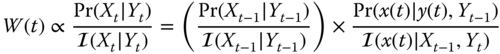
where ![]() means “proportional to.”
means “proportional to.”
Therefore, invoking the chain rule (above) at time ![]() and assuming the conditional independence of
and assuming the conditional independence of ![]() and the decomposition of Eq. 4.101, we obtain the recursion
and the decomposition of Eq. 4.101, we obtain the recursion
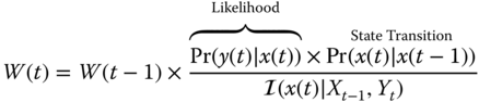
The generic sequential importance sampling solution is obtained by drawing particles from the importance (sampling) distribution, that is, for the ![]() th particle
th particle ![]() at time
at time ![]() , we have
, we have
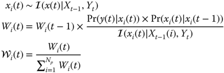
The resulting posterior is then estimated by
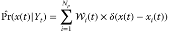
Note that it can also be shown that the estimate converges to the true posterior as
implying that the MC error variance decreases as the number of particles increase 32.
There are a variety of PF algorithms available based on the choice of the importance distribution 33–36. The most popular choice for the distribution is the state transition prior:
This prior is defined in terms of the state‐space representation ![]() , which is dependent on the known excitation (
, which is dependent on the known excitation (![]() ) and process noise (
) and process noise (![]() ) statistics. For this implementation, we draw samples from the state transition distribution using the dynamic state‐space model driven by the process uncertainty
) statistics. For this implementation, we draw samples from the state transition distribution using the dynamic state‐space model driven by the process uncertainty ![]() to generate the set of particles,
to generate the set of particles, ![]() for each
for each ![]() . So we see that in order to generate particles, we execute the state‐space simulation driving it with process noise
. So we see that in order to generate particles, we execute the state‐space simulation driving it with process noise ![]() for the
for the ![]() th particle.
th particle.
Substituting this choice into the expression for the weights gives

which is simply the likelihood distribution, since the priors cancel.
Note two properties for this choice of importance distribution. First, the weight does not use the most recent observation, ![]() and second, it does not use the past particles
and second, it does not use the past particles ![]() , but only the likelihood. This choice is easily implemented and updated by simply evaluating the measurement likelihood,
, but only the likelihood. This choice is easily implemented and updated by simply evaluating the measurement likelihood, ![]() for the sampled particle set.
for the sampled particle set.
This particular choice of importance distribution can lead to problems since the transition prior is not conditioned on the measurement data, especially the most recent. Failing to incorporate the latest available information from the most recent measurement to propose new values for the states leads to only a few particles having significant weights when their likelihood is calculated. The transition prior is a much broader distribution than the likelihood, indicating that only a few particles will be assigned a large weight. Thus, the algorithm will degenerate rapidly and lead to poor performance especially when data outliers occur or measurement noise is small. These conditions lead to a “mismatch” between the prior prediction and posterior distributions.
The basic “bootstrap” algorithm developed in 37 is one of the first practical implementations of this processor. It is the most heavily applied of all PF techniques due to its simplicity. We note that the importance weights are much simpler to evaluate with this approach that has been termed the bootstrap PF, the condensation PF, or the survival of the fittest algorithm 36 –38. Their practical implementation requires resampling of the particles to prevent degeneracy of the associated weights that increase in variance at each step, making it impossible to avoid the degradation. Resampling consists of processing the particles with their associated weights duplicating those of large weights (probabilities), while discarding those of small weights. In this way, only those particles of highest probabilities (importance) are retained, enabling a coalescence at the peaks of the resulting posterior distribution while mitigating the degradation. A measure based on the coefficient of variation is the effective particle sample size 32 :
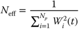
It is the underlying decision statistic such that when its value is less than a predetermined threshold resampling is performed (see [7] for more details).
The bootstrap technique is based on sequential sampling–importance–resampling (SIR) ideas and uses the transition prior as its underlying proposal distribution. The corresponding weight becomes quite simple and only depends on the likelihood; therefore, it is not even necessary to perform a sequential updating. Because the filter requires resampling to mitigate variance (weight) increases at each time‐step 37 , the new weights become

revealing that there is no need to save the likelihood (weight) from the previous step! With this in mind, we summarize the simple bootstrap PF algorithm in Table 4.7 . In order to achieve convergence, it is necessary to resample at every time‐step. In practice, however, many applications make the decision to resample based on the effective sample‐size metric of Eq. (4.108).
To construct the bootstrap PF, we assume the following: (i) ![]() is known; (ii)
is known; (ii) ![]() ,
, ![]() are known; (iii) samples can be generated using the process noise input and the state‐space model,
are known; (iii) samples can be generated using the process noise input and the state‐space model, ![]() ; (iv) the likelihood is available for point‐wise evaluation,
; (iv) the likelihood is available for point‐wise evaluation, ![]() based on the measurement model,
based on the measurement model, ![]() ; and (v) resampling is performed at every time‐step. We summarize the algorithm in Table 4.9.
; and (v) resampling is performed at every time‐step. We summarize the algorithm in Table 4.9.
To implement the algorithm, we have the following steps:
- Generate the initial state,
 .
. - Generate the process noise,
 .
. - Generate the particles,
 – the prediction‐step.
 - Generate the likelihood,
 using the current particle and measurement – the update step.
 - Resample the set of particles retaining and replicating those of highest weight (probability),
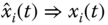 .
. - Generate the new set,
 with
with  .
.
Table 4.9 Bootstrap particle filter (PF) SIR algorithm.
| Initialize | |
| (Sample) | |
| Importance sampling | |
|
|
(State Transition) |
| Weight update | |
|
|
(Weight/Likelihood) |
| Weight normalization | |
 |
|
| Resampling decision | |
 |
(Effective Samples) |
| Resampling | |
| Distribution | |
 |
(Posterior Distribution) |
Next we revisit the nonlinear trajectory estimation problem of Jazwinski 3 and apply the simple bootstrap algorithm to demonstrate the PF solution using the state‐space SIR PF algorithm.

Figure 4.9 Nonlinear trajectory Bayesian estimation: Particle filter (PF) design. (a) State estimates: MAP, CM, UKF. (b) Predicted measurement estimates: MAP, CM, UKF. (c) Updated state instantaneous posterior distribution. (d) Predicted measurement instantaneous posterior distribution.
This completes the development of the most popular and simple PF technique. Next we consider some practical methods to evaluate PF performance.
4.3.7 Practical Bayesian Model‐Based Design: Performance Analysis
Pragmatic MC methods, even those that are model‐based, are specifically aimed at providing a reasonable estimate of the underlying posterior distribution; therefore, performance testing typically involves estimating just “how close” the estimated posterior is to the “true” posterior. However, within a Bayesian framework, this comparison of posteriors only provides a measure of relative performance, but does not indicate just how well the underlying model embedded in the processor “fits” the measured data. Nevertheless, these closeness methods are usually based on the Kullback–Leibler (KL) divergence measure 39 providing such an answer. However, in many cases, we do not know the true posterior, and therefore, we must resort to other means of assessing performance such as evaluating MSE or more generally checking the validity of the model by evaluating samples generated by the prediction or the likelihood cumulative distribution to determine whether or not the resulting sequences have evolved from a uniform distribution and are i.i.d (see 7 ) – analogous to a whiteness test for Gaussian sequences.
Thus, PFs are essentially sequential estimators of the posterior distribution employing a variety of embedded models to achieve meaningful estimates. In contrast to the Kalman filter designs, which are typically based on Gaussian assumptions, the PFs have no such constraints per se. Clearly, when noise is additive Gaussian, then statistical tests can also be performed based on the innovations or residual sequences resulting from the PF estimates (MAP, ML, CM) inferred from the estimated posterior distribution. In what might be termed “sanity testing,” the classical methods employ the basic statistical philosophy that “if all of the signal information has been removed (explained) from the measurement data, then the residuals (i.e. innovations or prediction error) should be uncorrelated,” that is, the model fits the data and all that remains is a white or uncorrelated residual (innovations) sequence. Therefore, performing the zero‐mean, whiteness testing as well as checking the normalized MSE of the state vector (and/or innovations) given by

are the basic (first) steps that can be undertaken to ensure that the models have been implemented properly and the processors have been “tuned.” Here the normalized MSE range is ![]() NMSE
NMSE![]() .
.
Also as before, simple ensemble statistics can be employed to provide an average solution enabling us to generate expected results. This approach is viable even for the PF, assuming we have a “truth model” (or data ensemble) available for our designs. As discussed in 7 , the performance analysis of the PF is best achieved by combining both simulated and actual measurement data possibly obtained during a calibration phase of the implementation. In this approach, the data are preprocessed and the truth model adjusted to reflect a set of predictive parameters that are then extracted and used to “parameterize” the underlying state‐space (or other) representation of the process under investigation. Once the models and parameters are selected, then ensemble runs can be performed; terms such as initial states, covariances, and noise statistics (means, covariances, etc.) can then be adjusted to “tune” the processor. Here classical statistics (e.g. zero‐mean/whiteness and WSSR testing) can help in the tuning phase. Once tuned, the processor is then applied to the raw measurement data, and ensemble statistics are estimated to provide a thorough analysis of the processor performance.
Much effort has been devoted to the validation problem with the most significant results evolving from the information theoretical point of view 40. Following this approach, we start with the basic ideas and converge to a reasonable solution to the distribution validation problem 40 ,41. Since many processors are expressed in terms of their “estimated” probability distributions, quality or “goodness” can be evaluated by its similarity to the true underlying probability distribution generating the measured data 42.
Suppose ![]() is the true posterior PMF and
is the true posterior PMF and ![]() is the estimated (particle) distribution, then the Kullback–Leibler information quantity of the true distribution relative to the estimated is defined by 43,44
is the estimated (particle) distribution, then the Kullback–Leibler information quantity of the true distribution relative to the estimated is defined by 43,44
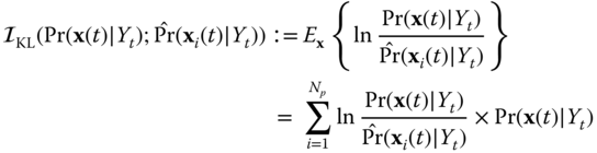
The KL satisfies its most important property from a distribution comparison viewpoint – when the true distribution and its estimate are close (or identical), then the information quantity is
This property infers that as the estimated posterior distribution approaches the true distribution, then the value of the KL approaches zero (minimum).
However, our interest lies in comparing two probability distributions to determine “how close” they are to each other. Even though ![]() does quantify the difference between the true and estimated distributions, unfortunately it is not a distance measure due to its lack of symmetry. However, the Kullback divergence (KD) defined by a combination of
does quantify the difference between the true and estimated distributions, unfortunately it is not a distance measure due to its lack of symmetry. However, the Kullback divergence (KD) defined by a combination of ![]() for this case is defined by
for this case is defined by

provides the distance metric indicating “how close” the estimated posterior is to the true distribution or, from our perspective, “how well does it approximate” the true. Thus, the KD is a very important metric that can be applied to assess the performance of Bayesian processors, providing a measure between the true and estimated posterior distributions.
If we have a “truth model,” then its corresponding probability surface is analogous to the PF surface and can be generated through an ensemble simulation with values of the probabilities selected that correspond to the true state values at ![]() (see 7
for details). An even simpler technique for nonanalytic distributions is to synthesize perturbed (low noise covariances) states generated by the model at each point in index (time) and estimate its histogram by kernel density smoothers directly to obtain an estimate of
(see 7
for details). An even simpler technique for nonanalytic distributions is to synthesize perturbed (low noise covariances) states generated by the model at each point in index (time) and estimate its histogram by kernel density smoothers directly to obtain an estimate of ![]() enabling the fact that the KD can now be approximated for a given realization by
enabling the fact that the KD can now be approximated for a given realization by

The implementation of the Kullback–Leibler divergence approach (state component‐wise) is
- Generate samples from the state “truth model”:
 .
. - Estimate the corresponding state truth model distribution:
 using the kernel density smoother.
 - Estimate the corresponding posterior distribution:
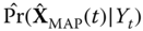 from the PF estimates
  .
. - Calculate the Kullback–Leibler divergence:
 .
. - Determine if
 for PF performance.
Before we close this section, we briefly mention a similar metric for comparing probability distributions – the Hellinger distance. The HD evolved from measure theory and is a true distance metric satisfying all of the required properties 45,46. It is a metric that can also be used to compare the similarity of two probability distributions with its values lying between zero and unity, that is, ![]() eliminating the question of “what is the closeness of KD to zero.”
eliminating the question of “what is the closeness of KD to zero.”
It provides a “scaled metric” similar to the “unscaled” Kullback–Leibler divergence providing a reasonable calculation to compare or evaluate overall performance.
For PF design/analysis, the corresponding Hellinger distance is specified by
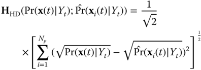
Using the truth model as before for the KD and its corresponding probability surface, the values of the probabilities selected correspond to the “true state” probabilities at ![]() can be approximated for a given realization by
can be approximated for a given realization by
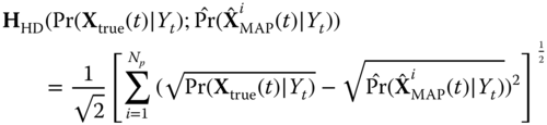
Consider the following example illustrating both Kullback–Leibler divergence and Hellinger distance metrics applied to the PF design for the trajectory estimation problem.

Figure 4.10 PMF data: Kullback–Leibler divergence and Hellinger distance calculations for the nonlinear trajectory estimation problem over  ‐member ensemble. (a) Measurement PMF ensemble. (b) State PMF ensemble. (c) KL‐divergence measurement median/mean (KD = 0.001 24/0.001 30). (d) KL‐divergence state median/mean (KD = 0.001 44/0.001 46) (e) HD‐distance measurement median/mean (HD = 0.0176/0.0178). (f) HD‐distance state median/mean (HD = 0.0189/0.0189).
This completes the section. Next we discuss an application of nonlinear filtering to a tracking problem.
4.4 Case Study: 2D‐Tracking Problem
In this section, we investigate the design of nonlinear MBP to solve a two‐dimensional (2D) tracking problem. The hypothetical scenario discussed will demonstrate the applicability of these processors to solve such a problem. It could easily be extrapolated to many other problems in nature (e.g. air control operations, position estimation) and develops the “basic” thinking behind constructing such a problem and solution.
Let us investigate the tracking of a large tanker entering a busy harbor with a prescribed navigation path. In this case, the pilot of the vessel must adhere strictly to the path that has been filed with the harbor master (controller). Here we assume that the ship has a transponder frequently signaling accurate information about its current position. The objective is to safely dock the tanker without any “traffic” incidents. We observe that the ship's path should track the prescribed trajectory (Cartesian coordinates) shown in Figure 4.11 with the corresponding instantaneous ![]() ‐positions (vs time) shown as well.
‐positions (vs time) shown as well.
Our fictitious measurement instrument (e.g. low ground clutter phased array radar or a GPS satellite communications receiver) is assumed to instantly report on the tanker position in bearing and range with high accuracy, that is, the measurements are given by

We use the state‐space formulation for a constant velocity model with state vector defined in terms of the physical variables as ![]() along with the incremental velocity input as
along with the incremental velocity input as ![]() .
.
Using this information (as before), the entire system can be represented as a Gauss–Markov model with the noise sources representing uncertainties in the states and measurements. Thus, we have the equations of motion given by
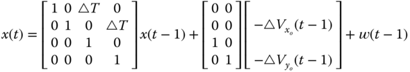
with the corresponding measurement model given by

for ![]() and
and ![]() .
.
The MATLAB software was used to simulate this Gauss–Markov system for the tanker path, and the results are shown in Figure 4.11
. In this scenario, we assume the instrument is capable of making measurements every ![]() hour with a bearing precision of
hour with a bearing precision of ![]() and a range precision of
and a range precision of ![]() nm (or equivalently
nm (or equivalently ![]() ]. The model uncertainty was represented by
]. The model uncertainty was represented by ![]() . An impulse‐incremental step change in velocity, e.g.
. An impulse‐incremental step change in velocity, e.g. ![]() going from
going from ![]() to
to ![]() is an incremental change of
is an incremental change of ![]() corresponding to
corresponding to ![]() knot and
knot and ![]() knot. These impulses (changes) occur at time fiducials of
knot. These impulses (changes) occur at time fiducials of ![]() hours corresponding to the filed harbor path depicted in the figure. Note that the velocity changes are impulses of height (
hours corresponding to the filed harbor path depicted in the figure. Note that the velocity changes are impulses of height (![]() ) corresponding to a known deterministic input,
) corresponding to a known deterministic input, ![]() . These changes relate physically to instantaneous direction changes of the tanker and create the path change in the constant velocity model.
. These changes relate physically to instantaneous direction changes of the tanker and create the path change in the constant velocity model.
The simulated bearing measurements are generated using the initial conditions ![]() and
and ![]() with the corresponding initial covariance given by
with the corresponding initial covariance given by ![]() . The EKF algorithm of Table 4.6
is implemented using these model parameters and the following Jacobian matrices derived from the Gauss–Markov model above:
. The EKF algorithm of Table 4.6
is implemented using these model parameters and the following Jacobian matrices derived from the Gauss–Markov model above:

The EKF, IEKF, and LZKF were run under the constraint that all of the a priori information for the tanker harbor path is “known.” Each of the processors performed almost identically with a typical single realization output shown for the EKF in Figure 4.12. In Figure 4.12
a,b we observe the estimated states ![]() ,
, ![]() ,
, ![]() ,
, ![]() . Note that the velocities are piecewise constant functions with step changes corresponding to the impulsive incremental velocities. The filtered measurements bearing (
. Note that the velocities are piecewise constant functions with step changes corresponding to the impulsive incremental velocities. The filtered measurements bearing (![]() out) and range (
out) and range (![]() out) are shown in Figure 4.12
c with the resulting innovations zero‐mean/whiteness tests depicted in (d). The processor is clearly tuned with bearing and range innovations zero‐mean and white (
out) are shown in Figure 4.12
c with the resulting innovations zero‐mean/whiteness tests depicted in (d). The processor is clearly tuned with bearing and range innovations zero‐mean and white (![]() /
/![]() out) and (
out) and (![]() /
/![]() out), respectively. This result is not unexpected, since all of the a priori information is given including the precise incremental velocity input,
out), respectively. This result is not unexpected, since all of the a priori information is given including the precise incremental velocity input, ![]() . An ensemble of 101 realizations of the estimator was run by generating random initial condition estimates from the Gaussian assumption. The 101‐realization ensemble averaged estimates closely follow the results shown in the figure with the zero‐mean/whiteness tests (
. An ensemble of 101 realizations of the estimator was run by generating random initial condition estimates from the Gaussian assumption. The 101‐realization ensemble averaged estimates closely follow the results shown in the figure with the zero‐mean/whiteness tests (![]() /
/![]() out), (
out), (![]() /
/![]() out) slightly worse.
out) slightly worse.
Next, we investigate the usual case where all of the information is known a priori except the impulsive incremental velocity changes represented by the deterministic input. Note that without the input, the processor cannot respond instantaneously to the velocity changes and therefore will lag (in time) behind in predicting the tanker path. The solution to this problem requires a joint estimation of the states and the unknown input, which is really a solution to a deconvolution problem 2
. It is also a problem that is ill‐conditioned especially, since ![]() is impulsive.
is impulsive.
In any case we ran the nonlinear KF algorithms over the simulated data, and the best results were obtained using the LZKF. This is expected, since we used the exact state reference trajectories, but not the input. Note that the other nonlinear KF has no knowledge of this trajectory inhibiting their performance in this problem. The results are shown in Figure 4.13 where we observe the state estimates as before. We note that the position estimates (![]() out,
out, ![]() out) appear reasonable, primarily because of the reference trajectories. The LZKF is able to compensate for the unknown impulsive input with a slight lag as shown at each of the fiducials. The velocity estimates (
out) appear reasonable, primarily because of the reference trajectories. The LZKF is able to compensate for the unknown impulsive input with a slight lag as shown at each of the fiducials. The velocity estimates (![]() out,
out, ![]() out) are actually low‐pass versions of the true velocities caused by the slower LZKF response even with the exact step changes available. These lags are more vividly shown in the bearing estimate of Figure 4.13
c, which shows the processor has great difficulty with the instantaneous velocity changes in bearing (
out) are actually low‐pass versions of the true velocities caused by the slower LZKF response even with the exact step changes available. These lags are more vividly shown in the bearing estimate of Figure 4.13
c, which shows the processor has great difficulty with the instantaneous velocity changes in bearing (![]() out). The range (
out). The range (![]() out) appears insensitive to this lack of knowledge primarily because the
out) appears insensitive to this lack of knowledge primarily because the ![]() ‐position estimates are good and do not have step changes like the velocity for the LZKF to track. Both processors are not optimal and the innovations sequences are zero‐mean but not white (
‐position estimates are good and do not have step changes like the velocity for the LZKF to track. Both processors are not optimal and the innovations sequences are zero‐mean but not white (![]() /
/![]() out), (
out), (![]() /
/![]() out).
out).
We also designed the UKF to investigate its performance on this problem and its results were quite good2 as shown in Figure 4.14. The processor does not perform a model linearization but a statistical linearization instead; it is clear from the figure that it performs better than any of the other processors for this problem. In Figure 4.14
a–d, we see that the ![]() position estimates “track” the data very well, while the
position estimates “track” the data very well, while the ![]() ‐velocity estimates are somewhat nosier due to the abrupt changes (steps) in tuning values of the process noise covariance terms. In order to be able to track the step changes, the process noise covariance could be increased even further at the cost of nosier estimates. The UKF tracks the estimated bearing and range reasonably well as shown in figure with a slight loss of bearing track toward the end of the time sequence. These results are demonstrated by the zero‐mean/whiteness test results of the corresponding innovations sequences. The bearing innovations statistics are
‐velocity estimates are somewhat nosier due to the abrupt changes (steps) in tuning values of the process noise covariance terms. In order to be able to track the step changes, the process noise covariance could be increased even further at the cost of nosier estimates. The UKF tracks the estimated bearing and range reasonably well as shown in figure with a slight loss of bearing track toward the end of the time sequence. These results are demonstrated by the zero‐mean/whiteness test results of the corresponding innovations sequences. The bearing innovations statistics are ![]() and
and ![]() out and the corresponding range innovations statistics given by
out and the corresponding range innovations statistics given by ![]() and
and ![]() out. Both indicate a tuned processor. These are the best results of all of the nonlinear processors applied. This completes the case study.
out. Both indicate a tuned processor. These are the best results of all of the nonlinear processors applied. This completes the case study.
It is clear from this study that nonlinear processors can be “tuned” to give reasonable results especially when they are provided with accurate a priori information. If the a priori information is provided in terms of prescribed reference trajectories as in this hypothetical case study, then the LZKF appears to provide superior performance, but in the real‐world tracking problem, when this information on the target is not available, then the EKF and IEKF can be tuned to give reasonable results.
There are many variants possible for these processors to improve their performance whether it be in the form of improved coordinate systems 47–49 or in the form of a set of models each with its own independent processor 19 . One might also consider using estimator/smoothers as in the seismic case 14 because of the unknown impulsive input. This continues to be a challenging problem. The interested reader should consult Ref. 19 and the references cited therein for more details.
This completes the chapter on nonlinear state‐space‐based MBP. Next we consider the performance of parametrically adaptive schemes for MBP.
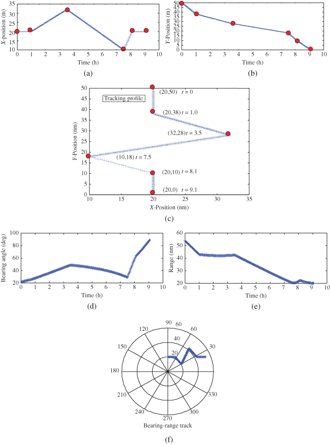
Figure 4.11 Tanker ground track geometry for the harbor docking application: (a) Instantaneous  ‐position (nm). (b) Instantaneous
  ‐position (nm). (c) Filed XY‐path (nm). (d) Instantaneous bearing (deg). (e) Instantaneous range (nm). (f) Polar bearing–range track from sensor measurement.

Figure 4.12 EKF design for harbor docking problem (input known). (a)  ‐position and velocity estimates with bounds
  out). (b)
  ‐position and velocity estimates with bounds
  and
and  out). (c) Bearing and range estimates with bounds
  and
and  out). (d) Innovations zero‐mean/whiteness tests for bearing (
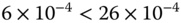 and
and  out) and range (
 and
and  out).
out).
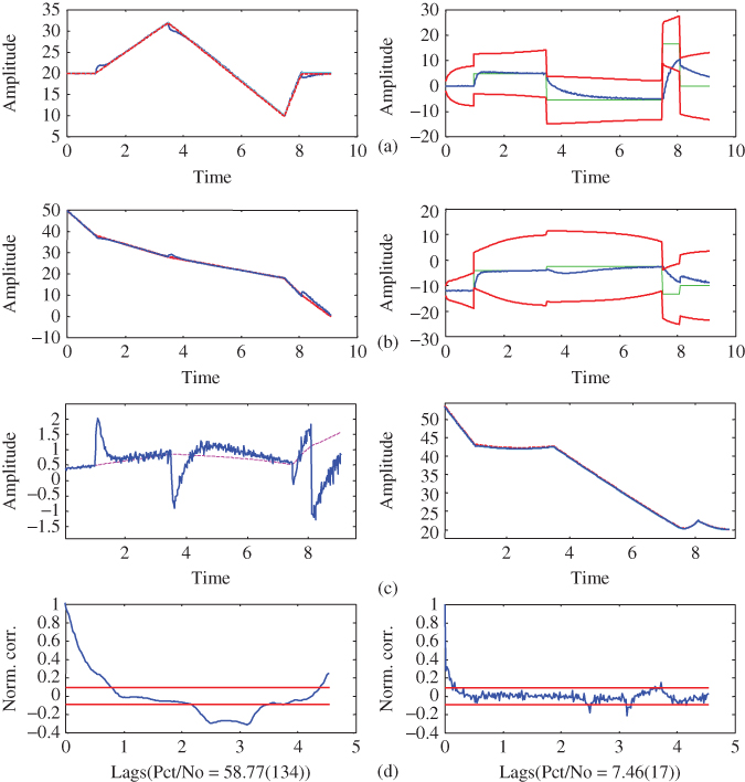
Figure 4.13 LZKF design for harbor docking problem (input known). (a)  ‐position and velocity estimates with bounds (
 and
and  out). (b)
  ‐position and velocity estimates with bounds (
 and
and  out). (c) Bearing and range estimates with bounds (
 and
and  out). (d) Innovations zero‐mean/whiteness tests for bearing (
 and
and  out) and range (
 and
and  out).
out).

Figure 4.14 UKF design for harbor docking problem (input unknown). (a)  ‐position estimate. (b)
  ‐position estimate. (c) X‐velocity estimate. (d) Y‐velocity estimate. (e) Bearing estimate (zero‐mean/whiteness:
  and
and  out). (f) Range estimate (zero‐mean/whiteness:
  and
and  out).
out).
4.5 Summary
In this chapter, we discussed the concepts of model‐based signal processing using state‐space models. We first introduced the recursive model‐based solution from a motivational perspective. We started with the linear, (time‐varying) Gauss–Markov model and developed a solution to the state estimation problem, leading to the well‐known LKF from the innovations perspective 3 . The objective was to basically introduce the processor from a pragmatic rather than theoretical approach 2 . Following this development, we investigated properties of the innovations sequence and eventually showed how they can be exploited to analyze processor performance that will be quite useful in subspace identification techniques to follow. With theory now in hand, we analyzed the properties of the “tuned” processor and showed how the MBP parameters can be used to achieve a minimum variance design.
Based on this fundamental theme, we progressed to nonlinear estimation problems and to the idea of linearization of the nonlinear state‐space model where we derive the LZKF. We then developed the EKF as a special case of the LZKF linearizing about the most currently available estimate. Next we investigated a further enhancement of the EKF by introducing a local iteration of the nonlinear measurement system. Here the processor is called the IEKF and was shown to produce improved estimates at a small computational cost in most cases.
Finally, we introduced the concepts of statistical signal processing from the Bayesian perspective using state‐space models. Two different paradigms for state estimation evolved: the UKF and the PF. The UKF employed a statistical rather than model linearization technique that yields superior statistical performance over the Kalman‐based methods, while the PF provides a complete Bayesian approach to the problem solution providing a nonparametric estimate of the required posterior distribution. Practical metrics were discussed to evaluate not only the nonlinear processors (LZKF, EKF, IEKF, UKF) but also Bayesian PF processor performance analysis. We summarized the results with a case study implementing a 2D‐tracking filter.
MATLAB Notes
MATLAB is a command‐oriented vector‐matrix package with a simple, yet effective command language featuring a wide variety of embedded ![]() language constructs, making it ideal for signal processing applications and graphics. Linear and nonlinear Kalman filter algorithms are available in the Control Systems (control) toolbox. Specifically, the LKF, EKF, UKF, and PF algorithms are available as well as state‐space simulators (LSIM). Also the System Identification (ident) provides simulation and analysis tools as well. MATLAB has a Statistics Toolbox that incorporates a large suite of PDFs and CDFs as well as “inverse” CDF functions ideal for simulation‐based algorithms. The mhsample command incorporate the Metropolis, Metropolis‐Hastings, and Metropolis independence samplers in a single command, while the Gibbs sampling approach is adequately represented by the more efficient slice sampler (slicesample). There are even specific “tools” for sampling as well as the inverse CDF method captured in the randsample command. PDF estimators include the usual histogram (hist) as well as the sophisticated kernel density estimator (ksdensity) offering a variety of kernel (window) functions (Gaussian, etc.). As yet no sequential algorithms are available.
language constructs, making it ideal for signal processing applications and graphics. Linear and nonlinear Kalman filter algorithms are available in the Control Systems (control) toolbox. Specifically, the LKF, EKF, UKF, and PF algorithms are available as well as state‐space simulators (LSIM). Also the System Identification (ident) provides simulation and analysis tools as well. MATLAB has a Statistics Toolbox that incorporates a large suite of PDFs and CDFs as well as “inverse” CDF functions ideal for simulation‐based algorithms. The mhsample command incorporate the Metropolis, Metropolis‐Hastings, and Metropolis independence samplers in a single command, while the Gibbs sampling approach is adequately represented by the more efficient slice sampler (slicesample). There are even specific “tools” for sampling as well as the inverse CDF method captured in the randsample command. PDF estimators include the usual histogram (hist) as well as the sophisticated kernel density estimator (ksdensity) offering a variety of kernel (window) functions (Gaussian, etc.). As yet no sequential algorithms are available.
In terms of statistical testing for particle filtering diagnostics, MATLAB offers the chi‐square “goodness‐of‐fit” test chi2gof as well as the Kolmogorov–Smirnov distribution test kstest. Residuals can be tested for whiteness using the Durbin–Watson test statistic dwtest, while “normality” is easily checked using the normplot command indicating the closeness of the test distribution to a Gaussian. Other statistics are also evaluated using the mean, moment, skewness, std, var, and kurtosis commands. Type help stats in MATLAB to get more details or go to the MathWorks website.
References
- 1 Kalman, R. (1960). A new approach to linear filtering and prediction problems. Trans. ASME J. Basic Eng. 82: 34–45.
- 2 Candy, J. (2006). Model‐Based Signal Processing. Hoboken, NJ: Wiley/IEEE Press.
- 3 Jazwinski, A. (1970). Stochastic Processes and Filtering Theory. New York: Academic Press.
- 4 Kailath, T. (1970). The innovations approach to detection and estimation theory. Proc. IEEE 58 (5): 680–695.
- 5 Kailath, T. (1981). Lectures on Kalman and Wiener Filtering Theory. New York: Springer.
- 6 Kailath, T., Sayed, A., and Hassibi, B. (2000). Linear Estimation. Englewood Cliffs, NJ: Prentice‐Hall.
- 7 Candy, J. (2016). Bayesian Signal Processing, Classical, Modern and Particle Filtering, 2e. Hoboken, NJ: Wiley/IEEE Press.
- 8 Anderson, B. and Moore, J. (1979). Optimal Filtering. Englewood Cliffs, NJ: Prentice‐Hall.
- 9 Wilsky, A.S. (1976). A survey of design methods for failure detection in dynamic systems. Automatica 12 (6): 601–611.
- 10 Mehra, R.K. and Peschon, J. (1971). An innovations approach to fault detection and diagnosis in dynamic systems. Automatica 7 (5): 637–640.
- 11 Martin, W.C. and Stubberud, A.R. (1976). The innovations process with application to identification. In: Control and Dynamic Systems (ed. C.T. Leondes), vol. 12, 173–258. New York: Academic Press.
- 12 Schweppe, F. (1973). Uncertain Dynamic Systems. Enegelwood Cliffs, NJ: Prentice‐Hall.
- 13 Maybeck, P. (1979). Stochastic Models, Estimation, and Control. New York: Academic Press.
- 14 Mendel, J. (1995). Lessons in Estimation Theory for Signal Processing, Communications and Control. Englewood Cliffs, NJ: Prentice‐Hall.
- 15 Bierman, G. (1977). Factorization Methods of Discrete Sequential Estimation. New York: Academic Press.
- 16 Sage, A. and Melsa, J. (1971). Estimation Theory with Applications to Communications and Control. New York: McGraw‐Hill.
- 17 Simon, D. (2006). Optimal State Estimation: Kalman,
 and Nonlinear Approaches. Hoboken, NJ: Wiley.
 - 18 Julier, S. and Uhlmann, J. (2004). Unscented filtering and nonlinear estimation. Proc. IEEE 92 (3): 401–422.
- 19 Bar‐Shalom, Y. and Li, X. (1993). Estimation and Tracking: Principles, Techniques and Software. Boston, MA: Artech House.
- 20 Candy, J. and Rozsa, R. (1980). Safeguards for a plutonium concentrator–an applied estimation approach. Automatica 16: 615–627.
- 21 Candy, J. and Sullivan, E. (1992). Ocean acoustic signal processing: a model‐based approach. J. Acoust. Soc. Am. 92 (6): 3185–3201.
- 22 Mendel, J.M., Kormylo, J., Aminzadeh, F. et al. (1981). A novel approach to seismic signal processing and modeling. Geophysics 46 (10): 1398–1414.
- 23 Sorenson, H. (ed.) (1983). Special issue on applications of Kalman filtering. IEEE Trans. Autom. Control AC‐28 (3): 253–427.
- 24 Julier, S., Uhlmann, J., and Durrant‐Whyte, H. (2000). A new method for the nonlinear transformation of means and covariances in filters and estimators. IEEE Trans. Autom. Control 45 (3): 477–482.
- 25 Julier, S. and Uhlmann, J. (1996). A General Method for Approximating Nonlinear Transformations of Probability Distributions. University of Oxford Report.
- 26 Haykin, S. and de Freitas, N. (eds.) (2004). Sequential state estimation: from Kalman filters to particle filters. Proc. IEEE 92 (3): 399–574.
- 27 Wan, E. and van der Merwe, R. (2000). The unscented Kalman filter for nonlinear estimation. Proceedings of IEEE Symposium 2000 on Adaptive Systems for Signal Processing, Communication and Control, Lake Louise, Alberta.
- 28 van der Merwe, R., Doucet, A., de Freitas, N., and Wan, E. (2000). The Unscented Particle Filter. Cambridge University Technical Report, CUED/F‐INFENG‐380.
- 29 Hogg, R. and Craig, A. (1970). Introduction to Mathematical Statistics. New York: MacMillan.
- 30 Ristic, B., Arulampalam, S., and Gordon, N. (2004). Beyond the Kalman Filter: Particle Filters for Tracking Applications. Boston, MA: Artech House.
- 31 Papoulis, A. (1965). Probability, Random Variables and Stochastic Processes. New York: McGraw‐Hill.
- 32 Liu, J. (2001). Monte Carlo Strategies in Scientific Computing. New York: Springer.
- 33 Arulampalam, M., Maskell, S., Gordon,N., and Clapp, T. (2002). A tutorial on particle filters for online nonlinear/non‐gaussian Bayesian tracking. IEEE Trans. Signal Process. 50 (2): 174–188.
- 34 Djuric, P., Kotecha, J., Zhang, J. et al. (2003). Particle filtering. IEEE Signal Process. Mag. 20 (5): 19–38.
- 35 Doucet, A., de Freitas, N., and Gordon, N. (2001). Sequential Monte Carlo Methods in Practice. New York: Springer.
- 36 Godsill, S. and Djuric, P. (2002). Special issue: Monte Carlo methods for statistical signal processing. IEEE Trans. Signal Proc. 50: 173–499.
- 37 Gordon, N., Salmond, D., and Smith, A. (1993). A novel approach to nonlinear non‐gaussian Bayesian state estimation. IEE Proc. F. 140 (2): 107–113.
- 38 Isard, M. and Blake, A. (1998). Condensation–conditional density propagation for visual tracking. Int. J. Comput. Vis. 29 (1): 5–28.
- 39 Gustafasson, F. (2000). Adaptive Filtering and Change Detection. Hoboken, NJ: Wiley.
- 40 Akaike, H. (1974). A new look at the statistical model identification. IEEE Trans. Autom. Control 19 (6): 716–723.
- 41 Sakamoto, Y., Ishiguro, M., and Kitagawa, G. (1986). Akaike Information Criterion Statistics (ed. D. Reidel). Boston, MA: Kluwer Academic.
- 42 Bhattacharyya, A. (1943). On a measure of divergence between two statistical populations defined by their probability distributions. Bull. Calcutta Math. Soc. 35: 99–109.
- 43 Kullback, S. and Leibler, R. (1951). On information and sufficiency. Ann. Math. Stat. 22: 79–86.
- 44 Kullback, S. (1978). Information Theory and Statistics. Gloucester, MA: Peter Smith.
- 45 Nikulin, M. (2001). Hellinger distance. In: Encyclopedia of Mathematics (ed. M. Hazewinkel). New York: Springer.
- 46 Beran, R. (1977). Minimum Hellinger distance estimates for parametric models. Ann. Stat. 5 (3): 445–463.
- 47 Aidala, V.J. and Hammel, S.M. (1983). Utilization of modified polar‐coordinates for bearings‐only tracking. IEEE Trans. Autom. Control AC‐28 (3): 283–294.
- 48 Aidala, V.J. (1979). Kalman filter behavior in bearings‐only velocity and position estimation. IEEE Trans. Aerosp. Electron. Syst. AES‐15: 29–39.
- 49 Candy, J.V. and Zicker, J.E. (1982). Deconvolution of Noisy Transient Signals: A Kalman Filtering Application. LLNL Rep., UCID‐87432, and Proceedings of CDC Conference, Orlando.
Problems
- 4.1
Derive the continuous‐time KF by starting with the discrete equations of Table 4.1
and using the following sampled‐data approximations:

- 4.2 Suppose we are given a continuous‐time Gauss–Markov model characterized by

and discrete (sampled) measurement model such that
 then
then
where the continuous process,
 , and
, and  with Gaussian initial conditions.
- (a) Determine the state mean (
 ) and covariance (
 ).
). - (b) Determine the measurement mean (
 ) and covariance (
 ).
). - (c) Develop the relationship between the continuous and discrete Gauss–Markov models based on the solution of the continuous state equations and approximation using a first‐order Taylor series for the state transition matrix,
 , and the associated system matrices.
 - (d) Derive the continuous–discrete KF using first‐difference approximations for derivatives and the discrete (sampled) system matrices derived above.
- (a) Determine the state mean (
- 4.3 The covariance correction equation of the KF algorithm is seldom used directly. Numerically, the covariance matrix
 must be positive semidefinite, but in the correction equation we are subtracting a matrix from a positive semidefinite matrix and cannot guarantee that the result will remain positive semidefinite (as it should be) because of roundoff and truncation errors. A solution to this problem is to replace the standard correction equation with the stabilized Joseph form, that is,

- (a) Derive the Joseph stabilized form.
- (b) Demonstrate that it is equivalent to the standard correction equation.
- 4.4 Prove that a necessary and sufficient condition for a linear KF to be optimal is that the corresponding innovations sequence is zero‐mean and white.
- 4.5 (a) (b) A bird watcher is counting the number of birds migrating to and from a particular nesting area. Suppose the number of migratory birds,
 , is modeled by a first‐order ARMA model:

while the number of resident birds is static, that is,
The number of resident birds is averaged, leading to the expression

- (a) Develop the two‐state Gauss–Markov model with initial values
 birds,
  birds,
  .
. - (b) Use the KF algorithm to estimate the number of resident and migrating birds in the nesting area for the data set
 , that is, what is
  ?
?
- (a) Develop the two‐state Gauss–Markov model with initial values
- 4.6 Suppose we are given a measurement device that not only acquires the current state but also the state delayed by one time‐step (multipath) such that

Derive the recursive form for this associated KF. (Hint: Recall from the properties of the state transition matrix that
 and
and  .)
.)- (a) Using the state transition matrix for discrete systems, find the relationship between
 and
and  in the Gauss–Markov model.
 - (b) Substitute this result into the measurement equation to obtain the usual form
What are the relations for

 and
and  in the new system?
 - (c) Derive the new statistics for
 (
( ,
,  ).
). - (d) Are
 and
and  correlated? If so, use the prediction form to develop the KF algorithm for this system.
- (a) Using the state transition matrix for discrete systems, find the relationship between
- 4.7 Develop the discrete linearized (perturbation) models for each of the following nonlinear systems 7
:
- Synchronous (unsteady) motor:

- (b) Duffing equation:

- (c) Van der Pol equation:

- (a) Hill equation:

- (a) Develop the LZKF.
- (b) Develop the EKF.
- (c) Develop the IEKF.
- Synchronous (unsteady) motor:
- 4.8 Suppose we are given the following discrete system:

with
 and
and  zero‐mean, white Gaussian with usual covariances,
  and
and  .
.- (a) Develop the LZKF for this process. (b) Develop the EKF for this process.
- (b) Develop the IEKF for this process.
- (c) Develop the UKF for this process.
- (d) Suppose the parameters
 and
and  are unknown. Develop the EKF such that the parameters are jointly estimated along with the states. (Hint: Augment the states and parameters to create a new state vector.)
- 4.9 Suppose we assume that a target is able to maneuver, that is, we assume that the target velocity satisfies a first‐order AR model given by

- (a) Develop the Cartesian tracking model for this process.
- (b) Develop the corresponding EKF assuming all parameters are known a priori.
- (c) Develop the corresponding EKF assuming
 is unknown.
 - (d) Develop the UKF for this process.
- 4.10 Consider the problem of estimating a random signal from an AM modulator characterized by

where
 is assumed to be a Gaussian random signal with power spectrum
also assume that the processes are contaminated with the usual additive noise sources:
 and
and  zero‐mean, white Gaussian with covariances,
  and
and  .
.- (a) Develop the continuous‐time Gauss–Markov model for this process.
- (b) Develop the corresponding discrete‐time Gauss–Markov model for this process using first differences.
- (c) Develop the KF.
- (d) Assume the carrier frequency,
 , is unknown. Develop the EKF for this process.
- 4.11
Let
 and
and  be i.i.d. with distribution
  . Suppose
  , then
- (a) What is the distribution of
 ,
,  ?
? - (b) Suppose
 and
and  , using the
  ‐point transformation what are the
  ‐points for
  ?
? - (c) What are the
 ‐points for
  ?
?
- (a) What is the distribution of
- 4.12
Suppose
 and
and  .
.
- (a) What is the distribution of
 ,
,  ?
? - (b) What is the Gaussian approximation of the mean and variance of
 ? (Hint: Use linearization.)
 - (c) What is the
 ‐point transformation and corresponding mean and variance estimates of
  ?
?
- (a) What is the distribution of
- 4.13
We are given a sequence of data and know it is Gaussian with an unknown mean and variance. The distribution is characterized by
 .
.
- (a) Formulate the problem in terms of a state‐space representation. (Hint: Assume that the measurements are modeled in the usual manner (scale by standard deviation and add mean to a
 “known” sequence, say
  .)
.) - (b) Using this model, develop the UKF technique to estimate the model parameters.
- (c) Synthesize a set of data of 2000 samples at a sampling interval
 with process covariance,
  and measurement noise of
  with
with  .
. - (d) Develop the UKF algorithm and apply it to this data and show the performance results (final parameter estimates, etc.). That is, find the best estimate of the parameters defined by
 using the UKF approach. Show the mathematical steps in developing the technique and construct a simple UKF to solve.
- (a) Formulate the problem in terms of a state‐space representation. (Hint: Assume that the measurements are modeled in the usual manner (scale by standard deviation and add mean to a
- 4.14
Given a sequence of Gaussian data (measurements) characterized by
 , find the best estimate of the parameters defined by
  using a “sequential” MC approach. Show the mathematical steps in developing the technique and construct a simple PF to solve the problem.
 - 4.15 Consider the following simple model
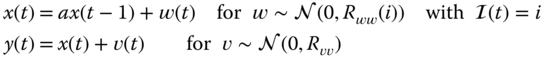
with

- (a) Suppose
 , what is the distribution,
  ?
? - (b) How would the marginal be estimated using a Kalman filter?
- (c) Develop a computational approach to bootstrap PF algorithm for this problem.
- (a) Suppose
- 4.16
Suppose we have two multivariate Gaussian distributions for the parameter vector,

- (a) Calculate the Kullback–Leibler (KL) distance metric,
 .
. - (b) Calculate the Hellinger (HD) distance metric,
 .
. - (c) Suppose
 . Recalculate the KL and HD for this case.
- (a) Calculate the Kullback–Leibler (KL) distance metric,
- 4.17 An aircraft flying over a region can use the terrain and an archival digital map to navigate. Measurements of the terrain elevation are collected in real time while the aircraft altitude over mean sea level is measured by a pressure meter with ground clearance measured by a radar altimeter. The measurement differences are used to estimate the terrain elevations and are compared to a digital elevation map to estimate the aircraft's position. The discrete navigation model is given by

where
 is the 2D‐position,
  is the terrain elevation measurement, the navigation system's output
  and
and  are the respective distance traveled and error drift during one time interval. The nonlinear function
  denotes the terrain database yielding terrain elevation outputs with
  the associated database errors and measurements. Both noises are assumed zero‐mean, Gaussian with known statistics, while the initial state is also Gaussian,
  .
.- (a) Based on this generic description, construct the bootstrap PF algorithm for this problem.
- (b) Suppose:
 ,
,  ,
,  ,
,  samples,
  . Simulate the aircraft measurements and apply the bootstrap algorithm to estimate the aircraft position.
- 4.18 Develop a suite of particle filters for the
 ‐circuit problem where the output voltage was given by

where
 is the initial voltage and
  is the resistance with
  the capacitance. The measurement equation for a voltmeter of gain
  is simply
Recall that for this circuit the parameters are:
 and
and  ,
,  ms,
ms,  V,
V,  , and the voltmeter is precise to within
  V. Then transforming the physical circuit model into state‐space form by defining
  ,
,  , and
, and  , we obtain
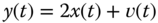
The process noise covariance is used to model the circuit parameter uncertainty with
 , since we assume standard deviations,
  ,
,  of
of  . Also,
  , since two standard deviations are
 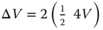 . We also assume initially that the state is
  , and that the input current is a step function of
  .
.With this in mind, we know that the optimal processor to estimate the state is the linear KF (Kalman filter).
- (a) After performing the simulation using the parameters above, construct a bootstrap PF and compare its performance to the optimal. How does it compare? Whiteness? Zero‐mean? State estimation error?
- (b) Let us assume that the circuit is malfunctioning and we do not precisely know the current values of
 . Construct a parameter estimator for
  using the EKF or UKF and compare its performance to the bootstrap and linearized PF.
- 4.19 We are asked to investigate the possibility of finding the range of a target using a hydrophone sensor array towed by an AUV assuming a near‐field target characterized by its spherical wavefront instead of the far‐field target of the previous problem using a plane wave model. The near‐field processor can be captured by a wavefront curvature scheme (see for more details) with process and measurement models (assuming that the parameters as well as the measurements are contaminated by additive white Gaussian noise). The following set of dynamic relations can be written succinctly as the Gauss–Markov wavefront curvature model as

where
 , and
, and  are the respective amplitude, target frequency, bearing, and range. The time delay at the
  th‐sensor and time
  is given in terms of the unknown parameters of
for
 the distance between the
  th sensor and reference range
  given by
- (a) Using this model, develop the bootstrap PF and UKF processors for this problem. Assume we would like to estimate the target bearing, frequency, and range (
 .
. - (b) Perform a simulation with initial parameters
 km,
km,  Hz, and
  and true parameters at
  km,
km,  Hz, and
  ,
,  .
. - (c) Apply the bootstrap algorithm with and without “roughening” along with the UKF. Discuss processor performances and compare. Zero‐mean? Whiteness?
- (d) Implement the “optimal” PF processor using the EKF or UKF linearization. How does its performance compare?
- (a) Using this model, develop the bootstrap PF and UKF processors for this problem. Assume we would like to estimate the target bearing, frequency, and range (
- 4.20 Consider a bearings‐only tracking problem given by the state‐space model. The entire system can be represented as an approximate Gauss–Markov model with the noise sources representing uncertainties in the states and measurements. The equations of motion given by
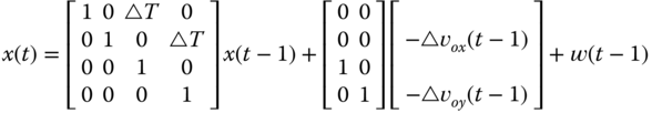
with the nonlinear sensor model given by

for
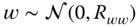 and
and  .
.- (a) Using this model, develop the bootstrap PF and UKF processors for this problem. Assume we would like to estimate the target bearing, frequency, and range (
 .
. - (b) Perform a simulation with the following parameters: an impulse‐incremental step change (
 knot and
  knot) was initiated at 0.5 hour, resulting in a change of observer position and velocity depicted in the figure. The simulated bearing measurements are shown in Figure 5.6d. The initial conditions for the run were
  and
and  with the measurement noise covariance given by
  for
for  hour.
hour. - (c) Apply the bootstrap algorithm along with the UKF. Discuss processor performances and compare. Zero‐mean? Whiteness?
- (d) Implement the “optimal” PF processor using the EKF or UKF linearization. How does its performance compare?
- (a) Using this model, develop the bootstrap PF and UKF processors for this problem. Assume we would like to estimate the target bearing, frequency, and range (