5
Parametrically Adaptive Processors
5.1 Introduction
The model‐based approach to the parameter estimation/system identification problem 1–4 is based on the decomposition of the joint posterior distributions that incorporate both dynamic state and parameter variables. From this formulation, the following problems evolve: joint state/parameter estimation; state estimation; and parameter (fixed and/or dynamic) estimation. The state estimation problem was discussed in the previous chapters. However, the most common problem found in the current literature is the parameter estimation problem that can be solved “off‐line” using batch approaches (maximum entropy, maximum likelihood, minimum variance, least squares, etc.) or “on‐line” using the recursive identification approach, the stochastic Monte Carlo approach and for that matter almost any (deterministic) optimization technique 5,6. These on‐line approaches follow the classical (EKF), modern (UKF), and the sequential Monte Carlo particle filter (PF). However, it still appears that there is no universally accepted technique to solve this problem especially for fixed parameters 7–9.
From the pragmatic perspective, the most useful problem is the joint state/parameter estimation problem, since it evolves quite naturally from the fact that a model is developed to solve the basic state estimation problem and it is found that its inherent parameters are poorly specified, just bounded, or even unknown, inhibiting the performance of the processor. We call this problem the “joint” state/parameter estimation, since both states and parameters are estimated simultaneously (on‐line) and the resulting processor is termed parametrically adaptive 10. This terminology evolves because the inherent model parameters are adjusted sequentially as the measurement data becomes available.
In this chapter, we concentrate primarily on the joint state/parameter estimation problem and refer the interested reader to the wealth of literature available on this subject 7 –19. First, we precisely define the basic problem from the Bayesian perspective and then investigate the classical, modern, and particle approaches to its solution. We incorporate the nonlinear trajectory estimation problem of Jazwinski 20 used throughout as an example of a parametrically adaptive design. Next we briefly develop the prediction error approach constrained to a linear model (RC‐circuit) and then discuss a case study to demonstrate the approach.
5.2 Parametrically Adaptive Processors: Bayesian Approach
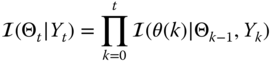
To be more precise, we start by defining the joint state/parametric estimation problem. We begin by formulating the Bayesian recursions in terms of the posterior distribution using Bayes' rule for decomposition, that is,
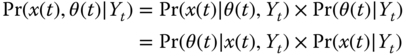
From this relation, we begin to “see” just how the variety of state and parameter estimation related problems evolve, that is,
- Optimize the state posterior:

- Optimize the parametric posterior:

- Optimize the joint state/parameter posterior:

Now if we proceed with the usual factorizations, we obtain the Bayesian decomposition for the state estimation problem as

Equivalently for the parameter estimation problem, we have

Now for the joint state/parameter estimation problem of Eq. 5.1, we can substitute the above equations to obtain the posterior decomposition of interest, that is,

This is the most common decomposition found in the literature 7
– 19
and leads to the maximization of the first term (in brackets) with respect to ![]() and the second with respect to
and the second with respect to ![]() 21,22.
21,22.
5.3 Parametrically Adaptive Processors: Nonlinear Kalman Filters
In this section, we develop parametrically adaptive processors for nonlinear state‐space systems. It is a joint state/parametric processor, since it estimates both the states and the embedded (unknown) model parameters. It is parametrically adaptive, since it adjusts or “adapts” the model parameters at each time step. The simplified structure of the classical extended Kalman filter state/parameter estimator is shown in Figure 5.1. We see the basic structure of the EKF with the augmented state vector that leads to two distinct, yet coupled subprocessors: a parameter estimator and a state estimator (filter). The parameter estimator provides estimates that are corrected by the corresponding innovations during each recursion. These estimates are then provided to the state estimator in order to update the model parameters used in the estimator. After both state and parameter estimates are calculated, a new measurement is processed and the procedure continues. In general, this processor can be considered to be a form of identifier, since system identification is typically concerned with the estimation of a model and its associated parameters from noisy measurement data. Usually, the model structure is predefined and then a parameter estimator is developed to “fit” parameters according to some error criterion. After completion or during this estimation, the quality of the estimates must be evaluated to decide if the processor performance is satisfactory or equivalently the model adequately represents the data. There are various types (criteria) of identifiers employing many different model (usually linear) structures 2– 4 . Here we are primarily concerned with joint estimation in which the models and parameters are nonlinear and discuss the linear case in Section 5.5. Thus, we will concentrate on developing parameter estimators capable of on‐line operations with nonlinear dynamics.

Figure 5.1 Parametrically adaptive processor structure illustrating the coupling between parameter and state estimators through the innovations and measurement sequences.
The solution to this joint estimation problem involves the augmentation of a parametric model (![]() ) along with the dynamic state (
) along with the dynamic state (![]() ) that embeds the parameters directly. Here the simple solution is to apply the same algorithm (LZKF, EKF, IEKF, UKF) with the original state vector replaced by the new “augmented” state
) that embeds the parameters directly. Here the simple solution is to apply the same algorithm (LZKF, EKF, IEKF, UKF) with the original state vector replaced by the new “augmented” state ![]() . The identical algorithm is then applied directly to the data. This is true for the classical and modern techniques, but not true for the MC‐based particle filters, since they must now draw particles from its priors and conditional parametric distributions. However, what happens if we do not have a direct physics‐based model for the parameters? The nonlinear processors require some characterization or parametric model to be embedded in the joint processor; therefore, we must have some way of providing a parametric representation, if a “physics‐based” model is not available.
. The identical algorithm is then applied directly to the data. This is true for the classical and modern techniques, but not true for the MC‐based particle filters, since they must now draw particles from its priors and conditional parametric distributions. However, what happens if we do not have a direct physics‐based model for the parameters? The nonlinear processors require some characterization or parametric model to be embedded in the joint processor; therefore, we must have some way of providing a parametric representation, if a “physics‐based” model is not available.
5.3.1 Parametric Models
Perhaps the most popular approach to this quandary is to use the so‐called “random walk” model that has evolved from the control/estimation area. This model essentially assumes a constant parameter (vector) ![]() with slight variations. In continuous time, a constant can be modeled by the differential equation
with slight variations. In continuous time, a constant can be modeled by the differential equation
here the solution is just the ![]() . Note that this differential equation is a state‐space formulation in
. Note that this differential equation is a state‐space formulation in ![]() enabling us to incorporate it directly into the overall dynamic model. Now if we artificially assign a Gaussian process noise term
enabling us to incorporate it directly into the overall dynamic model. Now if we artificially assign a Gaussian process noise term ![]() to excite the model, then a Wiener process or random walk (pseudo‐dynamic) model evolves. Providing a small variance to the noise source approximates small variations in the parameter, enabling it to “walk” in the underlying parameter space and converge to the true value. Since we typically concentrate on a sampled‐data system, we can discretize this representation using first differences (with
to excite the model, then a Wiener process or random walk (pseudo‐dynamic) model evolves. Providing a small variance to the noise source approximates small variations in the parameter, enabling it to “walk” in the underlying parameter space and converge to the true value. Since we typically concentrate on a sampled‐data system, we can discretize this representation using first differences (with ![]() ) and incorporate its corresponding mean/covariance propagation into our Gauss–Markov model, that is,
) and incorporate its corresponding mean/covariance propagation into our Gauss–Markov model, that is,

The process noise covariance ![]() controls the excursions of the random walk or equivalently the parameter space.
controls the excursions of the random walk or equivalently the parameter space.
We are primarily interested in physical systems that have parametric uncertainties that are well modeled by the random walk or other statistical variations. Of course, if the parametric relations are truly dynamic, then the joint approach incorporates these dynamics directly into the augmented state‐space model and yields an optimal filtering solution to this joint problem. Using these “artificial dynamics” is the approach employed in the classical LZKF, EKF, IEKF, modern UKF and other nonlinear state‐space techniques as well as the purely Bayesian processors (PF).
A popular variation of the random walk is based on incorporating the “forgetting factor” that has evolved from the system identification literature 1 and is called so because it controls the time constant of an inherent exponential window over the data. To see this, consider a squared‐error performance function defined by

where the window or weight ![]() is the forgetting factor that creates an exponentially decaying window of length, say
is the forgetting factor that creates an exponentially decaying window of length, say ![]() , in which the most recent data are weighted more than the past data. This follows from the following approximation 1
, 2
:
, in which the most recent data are weighted more than the past data. This follows from the following approximation 1
, 2
:
where ![]() is called the memory time constant that remains constant (approximately) over
is called the memory time constant that remains constant (approximately) over ![]() samples with typical choices between
samples with typical choices between ![]() in practice.
in practice.
The forgetting factor has been introduced into a variety of sequential algorithms in different roles. For instance, a direct implementation into the random walk model of Eq. 5.6 is 23
here ![]() affects the tracking speed of the updates providing a trade‐off between speed and noise attenuation. Setting
affects the tracking speed of the updates providing a trade‐off between speed and noise attenuation. Setting ![]() implies
implies ![]() an “infinite memory” while
an “infinite memory” while ![]() provides instantaneous response forgetting the entire past.
provides instantaneous response forgetting the entire past.
Thus, the forgetting factor introduces a certain amount of flexibility into the joint state/parameter estimation processors by enabling them to be more responsive to new data and therefore yielding improved signal estimates. The same effect is afforded by the process noise covariance matrix of Eq. 5.6 using an equivalent technique called “annealing.” The covariance matrix, usually assumed diagonal, is annealed toward zero using exponentially (decay) weighting (see 21 , 22 for more details).
Other variations of the parameter estimation models exist besides the statistical random walk model. For instance, similar to the random walk is a process called roughening, which is very similar in concept and is another simple pragmatic method of preventing the sample impoverishment problem for particle filters. It is a method suggested by Gordon et al. 15 and refined in 19 , termed particle “roughening,” which is similar to adding process noise to constant parameters when constructing a random walk model. It is useful in estimating embedded state‐space model parameters and can also be applied to the joint state/parameter estimation problem.
Roughening consists of adding random noise to each particle after resampling is accomplished, that is, the a posteriori particles are modified as
where ![]() and
and ![]() is a constant “tuning” parameter (e.g.
is a constant “tuning” parameter (e.g. ![]() ),
), ![]() is a vector of the maximum difference between particle components before roughening with the
is a vector of the maximum difference between particle components before roughening with the ![]() th element of
th element of ![]() given by
given by
5.3.2 Classical Joint State/Parametric Processors: Augmented Extended Kalman Filter
From our previous discussion in Chapter 4, it is clear that the extended Kalman filter can be applied to this problem directly through augmentation. We begin our analysis of the EKF as a joint processor closely following the approach of Ljung 24 for the linear problem discussed in Section 4.2. The general nonlinear parameter estimator structure can be derived directly from the EKF algorithm in Table 4.6.
The Bayesian solution to the classical problem is based on solving for the posterior (see Eq. 5.2) such that each of the required distributions is represented in terms of the EKF estimates. In the joint state/parameter estimation case, these distributions map simply by defining an augmented state vector ![]() to give (see Section 4.2)
to give (see Section 4.2)

where

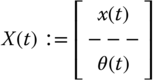
To develop the actual internal structure of the processor, we start with the EKF equations, augment them with the unknown parameters, and then investigate the resulting algorithm. We first define the composite state vector (as before) consisting of the original states, ![]() , and the unknown “augmented” parameters represented by
, and the unknown “augmented” parameters represented by ![]() , that is,
, that is,
where ![]() is the time index,
is the time index, ![]() , and
, and ![]() ,
, ![]() .
.
Substituting this augmented state vector into the EKF relations of Table 4.6, the following matrix partitions evolve as

where ![]() ,
, ![]() ,
, ![]() , and
, and ![]() .
.
This also leads to the partitioning of the corresponding gain
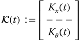
for ![]() ,
, ![]() , and
, and ![]() .
.
We must also partition the state and measurement predictions as equations, that is,

where the corresponding predicted measurement equation becomes
Here we have “implicitly” assumed that the parameters can be considered piecewise constant, ![]() or follow a random walk if we add process noise to this representation in the Gauss–Markov sense. However, if we do have process dynamics with linear or nonlinear models characterizing the parameters, then they will replace the random walk and the associated Jacobian.
or follow a random walk if we add process noise to this representation in the Gauss–Markov sense. However, if we do have process dynamics with linear or nonlinear models characterizing the parameters, then they will replace the random walk and the associated Jacobian.
Next, we consider the predicted error covariance
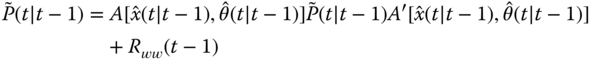
where ![]() is a block diagonal matrix consisting of the state and parameter covariance matrices:
is a block diagonal matrix consisting of the state and parameter covariance matrices: ![]() . The error covariance can be written in partitioned form using Eq. 5.14 and the following Jacobian process matrix:
. The error covariance can be written in partitioned form using Eq. 5.14 and the following Jacobian process matrix:

where
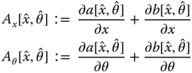
with ![]() .
.
Here is where the underlying random walk model enters the structure. The lower block rows of ![]() could be replaced by
could be replaced by ![]() , which enables a linear or nonlinear dynamic model to be embedded directly.
, which enables a linear or nonlinear dynamic model to be embedded directly.
Using these partitions, we can develop the parametrically adaptive processor directly from the EKF processor in this joint state and “parameter estimation” form. Substituting Eq. 5.19 into the EKF prediction covariance relation of Table 4.6 and using the partition defined in Eq. 5.14
, we obtain (suppressing the ![]() ,
, ![]() , time index
, time index ![]() notation for simplicity)
notation for simplicity)
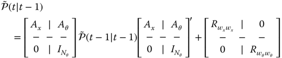
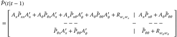
Expanding these equations, we obtain the following set of predicted covariance relations:
The innovations covariance follows from the EKF as
Now, we must use the partitions of ![]() above along with the measurement Jacobian
above along with the measurement Jacobian
where

with ![]()
The corresponding innovations covariance follows from Eqs. 5.23 and 5.24 as

or expanding
![]() . The gain of the EKF in Table 4.6 is calculated from these partitioned expressions as
. The gain of the EKF in Table 4.6 is calculated from these partitioned expressions as
or

where ![]() ,
, ![]() ,
, ![]() . With the gain determined, the corrected state/parameter estimates follow easily, since the innovations remain unchanged, that is,
. With the gain determined, the corrected state/parameter estimates follow easily, since the innovations remain unchanged, that is,
and therefore partitioning the corrected state equations, we have

Finally, the corrected covariance expression is easily derived from the following partitions:

Performing the indicated multiplications leads to the final expression

We summarize the parametrically adaptive EKF in predictor–corrector form in Table 5.1. We note that this algorithm is ![]() implemented in this manner – it merely evolves when the augmented state is processed using the “usual” EKF. Here we are just interested in the overall internal structure of the algorithm and the decompositions that evolve. This completes the development of the generic parametrically adaptive EKF processor. Clearly, this applies to any variants of the EKF including the LZKF.
implemented in this manner – it merely evolves when the augmented state is processed using the “usual” EKF. Here we are just interested in the overall internal structure of the algorithm and the decompositions that evolve. This completes the development of the generic parametrically adaptive EKF processor. Clearly, this applies to any variants of the EKF including the LZKF.
It is important to realize that besides its numerical implementation this processor is simply the EKF with an augmented state vector, thereby implicitly creating the partitions developed above. The implementation of these decomposed equations directly is not necessary – just augment the state with the unknown parameters, and it evolves naturally from the standard EKF algorithm of Table 4.6. The parametrically adaptive processor of Table 5.1
indicates where to locate the partitions. That is, suppose we would like to extract the submatrix, ![]() , but the EKF only provides the overall (
, but the EKF only provides the overall (![]() ) error covariance matrix,
) error covariance matrix, ![]() . However, locating the lower
. However, locating the lower ![]() submatrix of
submatrix of ![]() enables us to extract
enables us to extract ![]() directly.
directly.
Table 5.1 Augmented extended Kalman filter algorithm.
| Prediction | |
| (State) | |
|
|
(Parameter) |
 |
(State cov.) |
|
|
(Param. cov.) |
|
|
(Cross cov.) |
| Innovation | |
|
|
(Innovation) |
 |
(Innovation cov.) |
| Gain | |
|
|
(State Gain) |
|
|
(Parameter Gain) |
| Correction | |
|
|
(State) |
|
|
(Parameter) |
|
|
(State cov.) |
|
|
(Parameter cov.) |
|
|
(Cross cov.) |
| Initial Conditions | |
 |
|
Next, let us reconsider the nonlinear system example given in Chapter 4 and investigate the performance of the parametrically adaptive EKF processor.

Figure 5.2 Nonlinear (uncertain) trajectory estimation: parametrically adaptive EKF algorithm. (a) Estimated state and parameter no. 1. (b) Estimated parameter no. 2 and innovations. (c) Predicted measurement and zero‐mean/whiteness test ( and
and  out).
out).
As pointed out by Ljung and Soderstrom 2
, 24
, it is important to realize that the EKF is suboptimal as a parameter estimator compared to the recursive prediction error (RPE) method based on the Gauss–Newton (stochastic) descent algorithm (see Section 5.5
). Comparing the processors in this context, we see that if the gradient term ![]() is incorporated into the EKF (add this term to
is incorporated into the EKF (add this term to ![]() ), its convergence will be improved approaching the performance of the RPE algorithm (see Ljung 24
for details). Next, we consider the development of the “modern” approach using the unscented Kalman filter of Chapter 4.
), its convergence will be improved approaching the performance of the RPE algorithm (see Ljung 24
for details). Next, we consider the development of the “modern” approach using the unscented Kalman filter of Chapter 4.
5.3.3 Modern Joint State/Parametric Processor: Augmented Unscented Kalman Filter
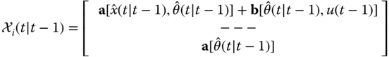
The modern unscented processor offers a similar representation as the extended processor detailed in section 5.3.2. Here, we briefly outline its structure for solution to the joint problem and apply it to the trajectory estimation problem for comparison. We again start with the augmented state vector defined initially by sigma‐points, that is,

![]() and
and ![]() ,
, ![]() .
.
Substituting this augmented state vector into the UKF relations of Table 4.8 yields the desired processor. We again draw the equivalences (as before):
where
With this in mind, it is possible to derive the internal structure of the UKF in a manner similar to that of the EKF. But we will not pursue that derivation here. We just note that the sigma‐points are also augmented to give

with the corresponding process noise covariance partitioned as

It also follows that the prediction step becomes
and in the multichannel (vector) measurement case we have that

Using the augmented state vector, we apply the “joint” approach to the trajectory estimation problem 20 and compare its performance to that of the EKF.
We also note in closing that a “dual” rather than “joint” approach has evolved in the literature. Originally developed as a bootstrap approach, it is constructed by two individual (decoupled) processors: one for the state estimator and one for the parameter estimator, which pass updated estimates back and forth to each other as they become available. This is a suboptimal methodology, but appears to perform quite well in some applications (see 21 , 22 for more details). This completes our discussion of the augmented modern UKF processor. Next we investigate the PF approach to solve the joint problem.

Figure 5.3 Nonlinear (uncertain) trajectory estimation: Parametrically adaptive UKF processor. (a) Estimated state and parameter no. 1. (b) Estimated parameter no. 2 and innovations. (c) Predicted measurement and zero‐mean/whiteness test ( and
and  out)
out)
5.4 Parametrically Adaptive Processors: Particle Filter
In this section, we briefly develop the sequential Monte Carlo approach to solve the joint state/parametric processing problem. There are a variety of ways to search the feasible space in pursuing solutions to the parameter estimation problem, but when states (or signals) must be extracted along with the parameters, then a solution to the joint estimation problem must follow as discussed before. One of the major problems that evolve is how to “model” the parameter evolution in order to provide an effective way to proceed with the search especially if there does not exist a physical model characterizing the parameters. The usual approach is to incorporate a random walk model as discussed previously, if the parameters are slowly varying.
5.4.1 Joint State/Parameter Estimation: Particle Filter
Here we are concerned with the joint estimation problem consisting of setting a prior for ![]() and augmenting the state vector to solve the joint estimation problem as defined above, thereby converting the parameter estimation problem to one of optimal filtering. Thus, confining our discussion to state‐space models and the Bayesian equivalence, we develop the Bayesian approach using the following relations:
and augmenting the state vector to solve the joint estimation problem as defined above, thereby converting the parameter estimation problem to one of optimal filtering. Thus, confining our discussion to state‐space models and the Bayesian equivalence, we develop the Bayesian approach using the following relations:

Here, we separate the state transition function into the individual vectors for illustrative purposes, but in reality (as we shall observe), they can be jointly coupled. The key idea is to develop the PF technique to estimate the joint posterior ![]() relying on the parametric posterior
relying on the parametric posterior ![]() in the Bayesian decomposition. We will follow the approach outlined in 17,25 starting with the full posterior distributions and proceeding to the filtering distributions.
in the Bayesian decomposition. We will follow the approach outlined in 17,25 starting with the full posterior distributions and proceeding to the filtering distributions.
Suppose it is possible to sample ![]() ‐particles,
‐particles, ![]() for
for ![]() from the joint posterior distribution where we define
from the joint posterior distribution where we define ![]() and
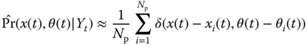
and ![]() . Then the corresponding empirical approximation of the joint posterior is given by
. Then the corresponding empirical approximation of the joint posterior is given by

and it follows directly that the filtering posterior is given by
Unfortunately, it is not possible to sample directly from the full joint posterior ![]() at any time
at any time ![]() . However, one approach to mitigate this problem is by using the importance sampling approach.
. However, one approach to mitigate this problem is by using the importance sampling approach.
Suppose we define a (full) importance distribution, ![]() such that
such that ![]() implies
implies ![]() , then we define the corresponding importance weight (as before) by
, then we define the corresponding importance weight (as before) by

From Bayes' rule, we have that the posterior can be expressed as

Thus, if ![]() ‐particles,
‐particles, ![]() , can be generated from the importance distribution
, can be generated from the importance distribution
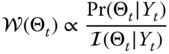
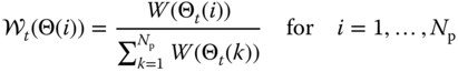
then the empirical distribution can be estimated and the resulting normalized weights specified by

to give the desired empirical distribution of Eq. 5.41 leading to the corresponding filtering distribution of Eq. 5.42.
If we have a state transition model available, then for a fixed parameter estimate, the state estimation problem is easily solved as in Chapter 4. Therefore, we will confine our discussion to the parameter posterior distribution estimation problem, that is, marginalizing the joint distribution with respect to the states (that have already been estimated) gives

and it follows that
Assuming that a set of particles can be generated from the importance distribution as ![]() , then we have the set of normalized weights
, then we have the set of normalized weights
which is the joint “batch” importance sampling solution when coupled with the dynamic state vectors.
The sequential form of this joint formulation follows directly as in Chapter 4. We start with the factored form of the importance distribution and focus on the full posterior ![]() , that is,
, that is,
with ![]() .
.
Assuming that this factorization can be expressed recursively in terms of the previous step, ![]() and extracting the
and extracting the ![]() th term gives
th term gives
or simply
With this in mind, the weight recursion becomes
Applying Bayes' rule to the posterior, we define

As before, in the state estimation problem, we must choose an importance distribution before we can construct the algorithm. The bootstrap approach can also be selected as the importance distribution leading to a simpler alternative with ![]() and the weight of Eq. 5.54 becomes the likelihood
and the weight of Eq. 5.54 becomes the likelihood
From the pragmatic perspective, we must consider some practical approaches to implement the processor for the joint problem. The first approach, when applicable, is to incorporate the random walk model when reasonable 17 . Another variant is to use the roughening model of Eq. 5.10 that “moves” the particles (after resampling) by adding a Gaussian sequence of specified variance.
This completes the discussion of the joint state/parameter estimation problem using the PF approach. Next we consider an example to illustrate the Bayesian approach.
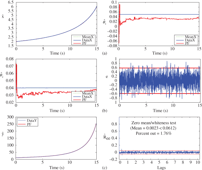
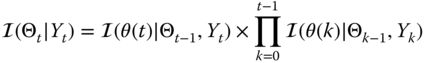
Figure 5.4 Nonlinear (uncertain) trajectory estimation: PF algorithm. (a) Estimated state and parameter no. 1. (b) Estimated parameter no. 2 and innovations. (c) Predicted measurement and zero‐mean/whiteness test ( and
and  out).
out).

Figure 5.5 PF posterior distribution estimation. (a) Estimated state posterior. (b) Parameter no. 1 posterior. (c) Parameter no. 2 posterior.

Figure 5.6 PF ensemble estimation for a  ‐member realizations. (a) Ensemble state estimate. (b) Ensemble parameter no. 1 estimate. (c) Ensemble parameter no. 2 estimate. (d) Ensemble measurement estimate.
5.5 Parametrically Adaptive Processors: Linear Kalman Filter
In this section, we briefly describe the recursive prediction error (RPE) approach to model‐based identification using the innovations model of Section 4.3 in parametric form. We follow the numerical optimization approach using the recursive Gauss–Newton algorithm developed by Ljung and Soderstrom 2 and available in MATLAB. This approach can also be considered “parametrically adaptive,” since it consists of both embedded state and parameter estimators as shown in Figure 5.1 .
Our task is to develop a parametrically adaptive version of the linear innovations state‐space model. The time‐invariant innovations model with parameter‐dependent (![]() ) system, input, output, and gain matrices:
) system, input, output, and gain matrices: ![]() ,
, ![]() ,
, ![]() ,
, ![]() is given by
is given by

For the parametrically adaptive algorithm, we transform the basic innovations structure to its equivalent prediction form.
Substituting for the innovations and collecting like terms, we obtain the prediction error model directly from the representation above, that is,

Comparing these models, we see that the following mappings occur:
Prediction error algorithms are developed from weighted quadratic criteria that evolve by minimizing the weighted sum‐squared error:
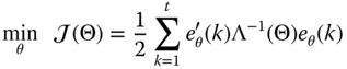
for the prediction error (innovations), ![]() and the innovations covariance (weighting) matrix,
and the innovations covariance (weighting) matrix, ![]() . The algorithm is developed by performing a second‐order Taylor series expansion about the parameter estimate,
. The algorithm is developed by performing a second‐order Taylor series expansion about the parameter estimate, ![]() , and applying the Gauss–Newton assumptions (e.g.
, and applying the Gauss–Newton assumptions (e.g. ![]() ) leading to the basic parametric recursion:
) leading to the basic parametric recursion:
where ![]() is the
is the ![]() gradient vector and
gradient vector and ![]() is the
is the ![]() Hessian matrix. As part of the RPE algorithm, we must perform these operations on the predictor; therefore, we define the gradient matrix by
Hessian matrix. As part of the RPE algorithm, we must perform these operations on the predictor; therefore, we define the gradient matrix by
Differentiating Eq. 5.59 using the chain rule,1 we obtain the gradient
using the gradient matrix from the definition above.
Defining the Hessian matrix as ![]() and substituting for the gradient in Eq. 5.60, we obtain the parameter vector recursion
and substituting for the gradient in Eq. 5.60, we obtain the parameter vector recursion
where ![]() is an
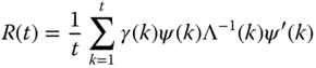
is an ![]() ‐weighting vector sequence. However, this does give us a recursive form, but it can be transformed to yield the desired result, that is, under the Gauss–Newton approximation, it has been shown 2
that the Hessian can be approximated by a weighted sample variance estimator of the form
‐weighting vector sequence. However, this does give us a recursive form, but it can be transformed to yield the desired result, that is, under the Gauss–Newton approximation, it has been shown 2
that the Hessian can be approximated by a weighted sample variance estimator of the form
which is easily placed in recursive form to give
Following the same arguments, the prediction error covariance can be placed in recursive form as well to give
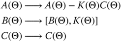
The ![]() ‐gradient matrix in terms of our innovations model is given by
‐gradient matrix in terms of our innovations model is given by
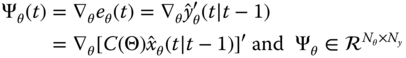
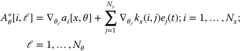
A matrix expansion of the gradient matrix with operations developed component‐wise is
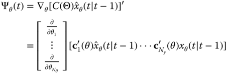
for ![]() and
and ![]() which can be expressed in a succinct notation as (see 10
for details)
which can be expressed in a succinct notation as (see 10
for details)

Define the following terms, which will ease the notational burden:
for ![]() , the state predictor gradient weighting matrix and
, the state predictor gradient weighting matrix and ![]() , the measurement gradient weighting matrix.
, the measurement gradient weighting matrix.
Thus, in terms of these definitions, we have
and therefore
Next we must develop an expression for ![]() by differentiating the predictor of Eq. 5.56, that is,
by differentiating the predictor of Eq. 5.56, that is,

Performing component‐wise derivatives, we differentiate the predictor as
Using our definitions for ![]() and
and ![]() , we have
, we have

Define the ![]() ‐matrix,
‐matrix,
Substituting component‐wise into Eq. 5.74 for each of the definitions (![]() ,
, ![]() ,
, ![]() ), we obtain
), we obtain

Now expanding over ![]() , we obtain the recursion for the state predictor gradient weighting matrix as
, we obtain the recursion for the state predictor gradient weighting matrix as
which completes the RPE algorithm applied to the innovations model. We summarize the algorithm in Table 5.2 using the simplified notation for clarity. That is, we use the Gauss–Newton approximations as before: ![]() ,
, ![]() ,
, ![]() and
and ![]() . We now apply this algorithm to the RC‐circuit problem.
. We now apply this algorithm to the RC‐circuit problem.
Table 5.2 Parametrically adaptive innovations model (RPE) algorithm.
| Prediction Error | |
| (Prediction Error) | |
|
|
(Prediction Error Covariance) |
|
|
(Hessian) |
| Parameter Estimation | |
|
|
(Parameter Update) |
| State Prediction | |
|
|
(State) |
|
|
(Measurement) |
| Gradient Prediction | |
|
|
(Weight) |
|
|
(Gradient) |
| Weighting Vector Sequence | |
| Initial Conditions | |

Figure 5.7 Parametrically adaptive innovations state‐space processor: RC‐circuit problem. (a) Noisy (dashed), true (thick dashed), and predicted (solid) measurements. (b) Innovations sequence ( out). (c) Zero‐mean/whiteness test (
 out).
out).
In practice, the innovations model is the usual approach taken for the linear parametrically adaptive state‐space processors. This completes the section on parametrically adaptive innovations model. Next we investigate a case study on the synthetic aperture tracking of an underwater source.
5.6 Case Study: Random Target Tracking
Synthetic aperture processing is well known in airborne radar, but not as familiar in sonar 26–31. The underlying idea in creating a synthetic aperture is to increase the array length by motion, thereby increasing the spatial resolution (bearing) and gain in SNR. It has been shown that for stationary targets the motion‐induced bearing estimates have smaller variances than that of a stationary array 29,32. Here we investigate the case of both array and target motion. We define the acoustic array space–time processing problem as follows:
GIVEN a set of noisy pressure‐field measurements from a horizontally towed array of ![]() ‐sensors in motion, FIND the “best” (minimum error variance) estimate of the target bearings.
‐sensors in motion, FIND the “best” (minimum error variance) estimate of the target bearings.
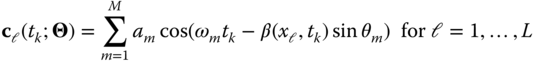
We use the following nonlinear pressure‐field measurement model for ![]() ‐monochromatic plane wave targets characterized by a corresponding set of temporal frequencies, bearings, and amplitudes,
‐monochromatic plane wave targets characterized by a corresponding set of temporal frequencies, bearings, and amplitudes, ![]() given by
given by

where ![]() ,
, ![]() is the wavenumber,
is the wavenumber, ![]() is the current spatial position along the
is the current spatial position along the ![]() ‐axis in meters,
‐axis in meters, ![]() is the tow speed in meter per second, and
is the tow speed in meter per second, and ![]() is the additive random noise. The inclusion of motion in the generalized wavenumber,
is the additive random noise. The inclusion of motion in the generalized wavenumber, ![]() , is critical to the improvement of the processing since the synthetic aperture effect is actually created through the motion itself and not simply the displacement.
, is critical to the improvement of the processing since the synthetic aperture effect is actually created through the motion itself and not simply the displacement.
If we further assume that the single sensor equation above is expanded to include an array of ![]() ‐sensors,
‐sensors, ![]() ,
, ![]() , then we obtain
, then we obtain

Since our hydrophone sensors measure the real part of the complex pressure‐field, the final nonlinear measurement model of the system can be written in compact vector form as
where ![]() , are the respective pressure‐field, measurement, and noise vectors and
, are the respective pressure‐field, measurement, and noise vectors and ![]() represents the target bearings. The corresponding vector measurement model
represents the target bearings. The corresponding vector measurement model
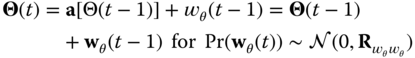
Since we model the bearings as a random walk emulating random target motion, then the Markovian state‐space model evolves from first differences as
Thus, the state‐space model is linear with no explicit dynamics; therefore, the process matrix ![]() (identity) and the relations are greatly simplified.
(identity) and the relations are greatly simplified.
Now let us see how a particle filter using the bootstrap approach can be constructed according to the generic algorithm of Table 4.9. For this problem, we assume the additive noise sources are Gaussian, so we can compare results to the performance of the approximate processor. We define the discrete notation, ![]() for the sampled‐data representation.
for the sampled‐data representation.
Let us cast this problem into the sequential Bayesian framework; that is, we would like to estimate the instantaneous posterior filtering distribution, ![]() , using the PF representation to be able to perform inferences and extract the target bearing estimates. Therefore, we have that the transition probability is given by (
, using the PF representation to be able to perform inferences and extract the target bearing estimates. Therefore, we have that the transition probability is given by (![]() )
)
or in terms of our state transition (bearings) model, we have
The corresponding likelihood is specified in terms of the measurement model (![]() ) as
) as
where we have used the notation: ![]() to specify the Gaussian distribution in random vector
to specify the Gaussian distribution in random vector ![]() . For our problem, we have that
. For our problem, we have that

with ![]() a constant,
a constant, ![]() and
and ![]() , the dynamic wavenumber expanded over the array. Thus, the PF SIR algorithm becomes
, the dynamic wavenumber expanded over the array. Thus, the PF SIR algorithm becomes
- Draw samples (particles) from the state transition distribution:

 ,
,  ;
; - Estimate the likelihood,
 with
with  and
and  the
the  th particle at the
  th bearing angle.
 - Update and normalize the weight:

- Resample:
 .
. - Estimate the instantaneous posterior:
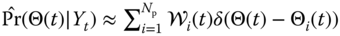 .
. - Perform the inference by estimating the corresponding statistics:
Consider the following simulation of the synthetic aperture using a four‐element, linear towed array with “moving” targets using the following parameters:
Target: Unity amplitudes with temporal frequency is 50 Hz, wavelength = 30 m, tow speed = 5 m ![]() Array: four (4) element linear towed array with 15 m spacing; Particle filter:
Array: four (4) element linear towed array with 15 m spacing; Particle filter: ![]() states (bearings),
states (bearings), ![]() sensors,
sensors, ![]() samples,
samples, ![]() particles/weights; SNR: is
particles/weights; SNR: is ![]() dB; Noise: white Gaussian with
dB; Noise: white Gaussian with ![]() ,
, ![]() ; Sampling interval is 0.005 second; Initial conditions: Bearings:
; Sampling interval is 0.005 second; Initial conditions: Bearings: ![]() ; Covariance:
; Covariance: ![]() .
.
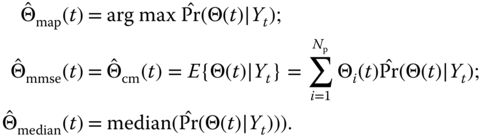
The array simulation was executed and the targets moved according to a random walk specified by the process noise and sensor array measurements with ![]() dB SNR. The results are shown in Figure 5.8, where we see the noisy synthesized bearings (left) and four (4) noisy sensor measurements at the moving array. The bearing (state) estimates are shown in Figure 5.9 where we observe the targets making a variety of course alterations. The PF is able to track the target motions quite well while we observe the unscented Kalman filter (UKF) 10
is unable to respond quickly enough and finally losing track completely for target no. 4. It should be noted that target no. 2 and target no. 4 “crossover” between 0.8 and 1.0 second. The PF loses these tracks during this time period getting them confused, but recovers by the one‐second time step. Both the MAP and CM estimates using the estimated posterior provide excellent tracking. Note that these bearing inputs would provide the raw data for an XY‐tracker 10
. The PF estimated or filtered measurements are shown in Figure 5.10. As expected the PF tracks the measurement data quite well, while the UKF is again in small error.
dB SNR. The results are shown in Figure 5.8, where we see the noisy synthesized bearings (left) and four (4) noisy sensor measurements at the moving array. The bearing (state) estimates are shown in Figure 5.9 where we observe the targets making a variety of course alterations. The PF is able to track the target motions quite well while we observe the unscented Kalman filter (UKF) 10
is unable to respond quickly enough and finally losing track completely for target no. 4. It should be noted that target no. 2 and target no. 4 “crossover” between 0.8 and 1.0 second. The PF loses these tracks during this time period getting them confused, but recovers by the one‐second time step. Both the MAP and CM estimates using the estimated posterior provide excellent tracking. Note that these bearing inputs would provide the raw data for an XY‐tracker 10
. The PF estimated or filtered measurements are shown in Figure 5.10. As expected the PF tracks the measurement data quite well, while the UKF is again in small error.
For performance analysis, we applied the usual “sanity tests.” From this perspective, the PF processor works well, since each measurement channel is zero‐mean and white with the WSSR lying below the threshold, indicating white innovations sequences demonstrating the tracking ability of the PF processor at least in a classical sense 10 (see Figure 5.11 and Table 5.3). The corresponding normalized root mean‐squared errors RMSE, median Kullback–Leibler divergence/Hellinger distance statistics for the bearing estimates are also shown in the table along with the measurements at each sensor. Estimating the KD/HD metrics for the measurements indicate a reasonable performance for both bearings and measurements.
The instantaneous posterior distributions for the bearing estimates are shown in Figure 5.12. Here we see the Gaussian nature of the bearing estimates generated by the random walk. Clearly, the PF performs quite well for this problem. Note also the capability of using the synthetic aperture, since we have only a four‐element sensor array, yet we are able to track four targets. Linear array theory implies with a static array that we should only be able to track ![]() three targets!
three targets!

Figure 5.8 Synthetic aperture sonar tracking problem: simulated target motion from initial bearings of  ,
,  ,
,  and
and  and array measurements (
 10 dB SNR).
Figure 5.9 Particle filter bearing estimates for four targets in random motion: PF bearing (state) estimates and simulated target tracks (UKF, conditional mean, MAP).

Figure 5.10 Particle filter predicted measurement estimates for four channel hydrophone sensor array.
Table 5.3 PF Performance towed array problem.
| Particle filter performance results | |||
| Parameter | RMSE | Median KLD | Median HD |
| Bearing no. 1 | 0.117 | 0.528 | 0.342 |
| Bearing no. 2 | 0.292 | 0.180 | 0.208 |
| Bearing no. 3 | 0.251 | 0.179 | 0.209 |
| Bearing no. 4 | 0.684 | 0.406 | 0.309 |
| Measurements | Median KLD | Median HD | |
| Sensor no. 1 | 0.066 | 0.139 | |
| Sensor no. 2 | 0.109 | 0.166 | |
| Sensor no. 3 | 0.259 | 0.275 | |
| Sensor no. 4 | 0.312 | 0.327 | |
| Innovations | Zero‐mean |
Whiteness | WSSR |
| Sensor no. 1 | 0.0102 | 5.47% | Below |
| Sensor no. 2 | 0.0136 | 1.56% | Below |
| Sensor no. 3 | 0.0057 | 5.47% | Below |
| Sensor no. 4 | 0.0132 | 2.34% | Below |

Figure 5.11 Particle filter classical “sanity” performance metrics: zero‐mean/whiteness tests for  ,
,  ,
,  and
and  targets as well the corresponding
  test.
test.

Figure 5.12 Particle filter instantaneous posterior bearing estimates: (a)  target no. 1 posterior; (b)
  target no. 2 posterior; (c)
  target no. 3; and (d)
  target no. 4.
In this case study, we have applied the unscented Kalman filter and the bootstrap PF to an ocean acoustic, synthetic aperture, towed array, target tracking problem to evaluate the performance of both the parametrically adaptive UKF and particle filtering techniques. The results are quite reasonable on this simulated data set.
5.7 Summary
In this chapter, we have discussed the development of joint Bayesian state/parametric processors. Starting with a brief introduction, we defined a variety of problems based on the joint posterior distribution ![]() and its decomposition. We focused on the joint problem of estimating both states and parameters simultaneously (on‐line) – a common problem of high interest. We then briefly showed that all that is necessary for this problem is to define an “augmented” state consisting of the original state variables along with the unknown parameters typically modeled by a random walk, when a dynamic parametric model is not available. This casts the joint problem into an optimal filtering framework. We then showed how this augmentation leads to a decomposition of the classical EKF processor and developed the “decomposed” form for illustrative purposes. The algorithm was implemented by executing the usual processor with the new augmented state vector embedded. We also extended this approach to both modern “unscented” and “particle‐based” processors, again only requiring the state augmentation procedure to implement. All of the processors required a random walk parametric model to function, while the particle filters could be implemented using the “roughening” (particle random walks) to track the parameters effectively. Next we discussed the recursive prediction error approach (RPE) and developed the solution for a specific linear, time‐invariant, state‐space model – the innovations model that will prove useful in subsequent subspace realization chapters to follow. Besides applying the nonlinear processors to the parametrically uncertain nonlinear trajectory estimation problem, we developed a case study for a synthetic aperture towed array and compared the modern UKF to the PF processors to complete the chapter 34–46.
and its decomposition. We focused on the joint problem of estimating both states and parameters simultaneously (on‐line) – a common problem of high interest. We then briefly showed that all that is necessary for this problem is to define an “augmented” state consisting of the original state variables along with the unknown parameters typically modeled by a random walk, when a dynamic parametric model is not available. This casts the joint problem into an optimal filtering framework. We then showed how this augmentation leads to a decomposition of the classical EKF processor and developed the “decomposed” form for illustrative purposes. The algorithm was implemented by executing the usual processor with the new augmented state vector embedded. We also extended this approach to both modern “unscented” and “particle‐based” processors, again only requiring the state augmentation procedure to implement. All of the processors required a random walk parametric model to function, while the particle filters could be implemented using the “roughening” (particle random walks) to track the parameters effectively. Next we discussed the recursive prediction error approach (RPE) and developed the solution for a specific linear, time‐invariant, state‐space model – the innovations model that will prove useful in subsequent subspace realization chapters to follow. Besides applying the nonlinear processors to the parametrically uncertain nonlinear trajectory estimation problem, we developed a case study for a synthetic aperture towed array and compared the modern UKF to the PF processors to complete the chapter 34–46.
MATLAB Notes
MATLAB has a variety of parametrically adaptive algorithms available in the Controls/Identification toolboxes. The linear Kalman filter (Kalman), extended Kalman filter (extendedKalmanFilter), and unscented Kalman filter (unscentedKalmanFilter) algorithms are available or as a set of commands: (predict) and (correct). The Identification toolbox has an implementation of the recursive prediction error method for a variety of model sets. The state‐space algorithms available are N4SID in the ident toolbox as well as the ekf, ukf, and pf of the control toolbox.
References
- 1 Ljung, L.J. (1999). System Identification: Theory for the User, 2e. Englewood Cliffs, NJ: Prentice‐Hall.
- 2 Ljung, L.J. and Soderstrom, T. (1983). Theory and Practice of Recursive Identification. Boston, MA: MIT Press.
- 3 Soderstrom, T. and Stoica, P. (1989). System Identification. Englewood Cliffs, NJ: Prentice‐Hall.
- 4 Norton, J.P. (1986). An Introduction to Identification. New York: Academic Press.
- 5 Liu, J. (2001). Monte Carlo Strategies in Scientific Computing. New York: Springer.
- 6 Cappe, O., Moulines, E., and Ryden, T. (2005). Inference in Hidden Markov Models. New York: Springer.
- 7 Liu, J. and West, M. (2001). Combined parameter and state estimation in simulation‐based filtering. In: Sequential Monte Carlo Methods in Practice, Chapter 10 (ed. A. Doucet, N. de Freitas, and N. Gordon), 197–223. New York: Springer.
- 8 Doucet, A., de Freitas, N., and Gordon, N. (2001). Sequential Monte Carlo Methods in Practice. New York: Springer.
- 9 Godsill, S. and Djuric, P. (2002). Special issue: Monte Carlo methods for statistical signal processing. IEEE Trans. Signal Process. 50: 173–499.
- 10 Candy, J. (2016). Bayesian Signal Processing: Classical, Modern and Particle Filtering Methods, 2e. Englewood Cliffs, NJ: Wiley/IEEE Press.
- 11 Cappe, O., Godsill, S., and Moulines, E. (2007). An overview of existing methods and recent advances in sequential Monte Carlo. Proc. IEEE 95 (5): 899–924.
- 12 Kitagawa, G. and Gersch, W. (1997). Smoothness Priors Analysis of Time Series. New York: Springer.
- 13 Kitagawa, G. (1998). Self‐organizing state space model. J. Am. Stat. Assoc. 97 (447): 1207–1215.
- 14 van der Merwe, R., Doucet, A., de Freitas, N., and Wan, E. (2000). The unscented particle filter. In: Advances in Neural Information Processing Systems, vol. 16. Cambridge, MA: MIT Press, Cambridge University Engineering Technical Report, CUED/F‐INFENG/TR 380.
- 15 Gordon, N., Salmond, D., and Smith, A. (1993). A novel approach to nonlinear non‐Gaussian Bayesian state estimation. IEE Proc. F. 140: 107–113.
- 16 Haykin, S. and de Freitas, N. (2004). Special issue: sequential state estimation: from Kalman filters to particle filters. Proc. IEEE 92 (3): 399–574.
- 17 Andrieu, C., Doucet, A., Singh, S., and Tadic, V. (2004). Particle methods for change detection, system identification and control. Proc. IEEE 92 (6): 423–468.
- 18 Haykin, S. (2001). Kalman Filtering and Neural Networks. New York: Wiley.
- 19 Simon, D. (2006). Optimal State Estimation: Kalman
 and Nonlinear Approaches. Englewood Cliffs, NJ: Wiley/IEEE Press.
 - 20 Jazwinski, A. (1970). Stochastic Processes and Filtering Theory. New York: Academic Press.
- 21 van der Merwe, R. (2004). Sigma‐point Kalman filters for probabilistic inference in dynamic state‐space models. PhD dissertation. OGI School of Science & Engineering, Oregon Health & Science University.
- 22 Nelson, A. (2000). Nonlinear estimation and modeling of noisy time‐series by Dual Kalman filtering methods. PhD dissertation. OGI School of Science & Engineering, Oregon Health & Science University.
- 23 Gustafsson, F. (2001). Adaptive Filtering and Change Detection. Englewood Cliffs, NJ: Wiley/IEEE Press.
- 24 Ljung, L. (1979). Asymptotic behavior of the extended Kalman filter as a parameter estimator for linear systems. IEEE Trans. Autom. Control AC‐24: 36–50.
- 25 Vermaak, J., Andrieu, C., Doucet, A., and Godsill, S. (2002). Particle methods for Bayesian modeling and enhancement of speech signals. IEEE Trans. Speech Audio Process. 10 (3): 173–185.
- 26 Williams, R. (1976). Creating an acoustic synthetic aperture in the ocean. J. Acoust. Soc. Am. 60: 60–73.
- 27 Yen, N. and Carey, W. (1976). Applications of synthetic aperture processing to towed array data. J. Acoust. Soc. Am. 60: 764–775.
- 28 Stergiopoulus, S. and Sullivan, E. (1976). Extended towed array processing by an overlap correlator. J. Acoust. Soc. Am. 86: 764–775.
- 29 Sullivan, E., Carey, W., and Stergiopoulus, S. (1992). Editorial in special issue on acoustic synthetic aperture processing. IEEE J. Ocean. Eng. 17: 1–7.
- 30 Ward, D., Lehmann, E., and Williamson, R. (2003). Particle filtering algorithm for tracking and acoustic source in a reverberant environment. IEEE Trans. Speech Audio Process. 11 (6): 826–836.
- 31 Orton, M. and Fitzgerald, W. (2002). Bayesian approach to tracking multiple targets using sensor arrays and particle filters. IEEE Trans. Signal Process. 50 (2): 216–223.
- 32 Sullivan, E. and Candy, J. (1997). Space‐time array processing: the model‐based approach. J. Acoust. Soc. Am. 102 (5): 2809–2820.
- 33 Gelb, A. (1975). Applied Optimal Estimation. Boston, MA: MIT Press.
- 34 Candy, J. (2007). Bootstrap particle filtering. IEEE Signal Process. Mag. 24 (4): 73–85.
- 35 Rajan, J., Rayner, P., and Godsill, S. (1997). Bayesian approach to parameter estimation and interpolation of time‐varying autoregressive processes using the Gibbs sampler. IEE Proc.‐Vis. Image Signal Process. 144 (4): 249–256.
- 36 Polson, N., Stroud, J., and Muller, P. (2002). Practical Filtering with Sequential Parameter Learning. University Chicago Technical Report, 1–18.
- 37 Andrieu, C., Doucet, A., Singh, S., and Tadic, V. (2004). Particle methods for change detection, system identification and control. Proc. IEEE 92 (3): 423–438.
- 38 Storvik, G. (2002). Particle filters in state space models with the presence of unknown static parameters. IEEE Trans. Signal Process. 50 (2): 281–289.
- 39 Djuric, P. (2001). Sequential estimation of signals under model uncertainty. In: Sequential Monte Carlo Methods in Practice, Chapter 18 (ed. A. Doucet, N. de Freitas, and N. Gordon), 381–400. New York: Springer.
- 40 Lee, D. and Chia, N. (2002). A particle algorithm for sequential Bayesian parameter estimation and model selection. IEEE Trans. Signal Process. 50 (2): 326–336.
- 41 Doucet, A. and Tadic, V. (2003). Parameter estimation in general state‐space models using particle methods. Ann. Inst. Stat. Math. 55 (2): 409–422.
- 42 Andrieu, C., Doucet, A., and Tadic, V. (2005). On‐line parameter estimation in general state‐space models. In: Proceedings of the 44th IEEE Conference on Decision and Control, 332–337.
- 43 Schoen, T. and Gustafsson, F. (2003). Particle Filters for System Identification of State‐Space Models Linear in Either Parameters or States. Linkoping University Report, LITH‐ISY‐R‐2518.
- 44 Faurre, P.L. (1976). Stochastic realization algorithms. In: System Identification: Advances and Case Studies (ed. R. Mehra and D. Lainiotis), 1–23. New York: Academic Press.
- 45 Tse, E. and Wiennert, H. (1979). Structure identification for multivariable systems. IEEE Trans. Autom. Control AC‐24: 36–50.
- 46 Bierman, G. (1977). Factorization Methods of Discrete Sequential Estimation. New York: Academic Press.
Problems
5.1 Suppose we are given the following innovations model (in steady state):

where ![]() is the zero‐mean, white innovations sequence with covariance,
is the zero‐mean, white innovations sequence with covariance, ![]() .
.
- (a) Derive the Wiener solution using the spectral factorization method of Section 2.4.
- (b) Develop the linear steady‐state KF for this model.
- (c) Develop the parametrically adaptive processor to estimate
 and
and  .
.
- 5.2 As stated in the chapter, the EKF convergence can be improved by incorporating a gain gradient term in the system Jacobian matrices, that is,

- (a) By partitioning the original
 Jacobian matrix,
  , derive the general “elemental” recursion, that is, show that
- (b) Suppose we would like to implement this modification, does there exist a numerical solution that could be used? If so, describe it.
- (a) By partitioning the original
- 5.3 Using the following scalar Gauss–Markov model

with the usual zero‐mean,
 and
and  covariances.
- (a) Let
 be scalars. Develop the EKF solution to estimate
  from noisy data.
 - (b) Can these algorithms be combined to “tune” the resulting hybrid processor?
- (a) Let
- 5.4 Suppose we are given the following structural model:

with the usual zero‐mean,
 and
and  covariances.
- (a) Convert this model into discrete‐time using first differences. Using central difference, create the discrete Gauss–Markov model. (Hint:
 .)
.) - (b) Suppose we would like to estimate the spring constant
 from noisy displacement measurements, develop the EKF to solve this problem.
 - (c) Transform the discrete Gauss–Markov model to the innovations representation.
- (d) Solve the parameter estimation problem using the innovations model; that is, develop the estimator of the spring constant.
- (a) Convert this model into discrete‐time using first differences. Using central difference, create the discrete Gauss–Markov model. (Hint:
- 5.5 Given the ARMAX model

with innovations covariance,
 :
:- (a) Write the expressions for the EKF in terms of the ARMAX model.
- (b) Write the expressions for the EKF in terms of the state‐space model.
- 5.6 Consider tracking a body falling freely through the atmosphere 33. We assume it is falling down in a straight line toward a radar. The state vector is defined by
 where
where  is the ballistic coefficient. The dynamics are defined by the state equations

where
 is the drag deceleration,
  is the acceleration of gravity (32.2),
  is the atmospheric density (with
  (
( density at sea level), and
  a decay constant (
 ). The corresponding measurement is given by
for
 . Initial values are
  ,
,  and
and  .
.- (a) Is this an EKF If so, write out the explicit algorithm in terms of the parametrically adaptive algorithm of this chapter.
- (b) Develop the EKF for this problem and perform the discrete simulation using MATLAB.
- (c) Develop the LZKF for this problem and perform the discrete simulation using MATLAB.
- (d) Develop the PF for this problem and perform the discrete simulation using MATLAB.
- 5.7 Parameter estimation can be performed directly when we are given a nonlinear measurement system such that
where
 and
and  and
and  ).
).- (a) From the a posteriori density,
 , derive the MAP estimator for
  .
. - (b) Expand
 in a Taylor series about
  and incorporate the first‐order approximation into the MAP estimator (approximate).
 - (c) Expand
 in a Taylor series about
  and incorporate the second‐order approximation into the MAP estimator (approximate).
 - (c) Develop an iterated version of both estimators in (b) and (c). How do they compare?
- (d) Use the parametrically adaptive formulation of this problem assuming the measurement model is time‐varying. Construct the EKF assuming that
 is modeled by a random walk. How does this processor compare to the iterated versions?
- (a) From the a posteriori density,
- 5.8 Suppose we are asked to solve a detection problem, that is, we must “decide” whether a signal is present or not according to the following binary hypothesis test:
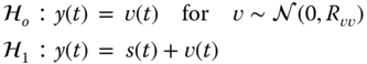
The signal is modeled by a Gauss–Markov model

- (a) Calculate the likelihood‐ratio defined by
where the measurement data set is defined by
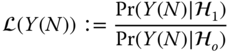
 . Calculate the corresponding threshold and construct the detector (binary hypothesis test).
 - (b) Suppose there is an unknown but deterministic parameter in the signal model, that is,
Construct the “composite” likelihood ratio for this case. Calculate the corresponding threshold and construct the detector (binary hypothesis test). (Hint: Use the EKF to jointly estimate the signal and parameter.)

- (c) Calculate a sequential form of the likelihood ratio above by letting the batch of measurements,
 . Calculate the corresponding threshold and construct the detector (binary hypothesis test). Note that there are two thresholds for this type of detector.
- (a) Calculate the likelihood‐ratio defined by
- 5.9 Angle modulated communications including both frequency modulation (FM) and phase modulation (PM) are basically nonlinear systems from the model‐based perspective. They are characterized by high bandwidth requirements, and their performance is outstanding in noisy environments. Both can be captured by the transmitted measurement model:

where
 is a constant,
  is the carrier frequency,
  and
and  are the deviation constants for the respective modulation systems, and of course,
  , is the message model. Demodulation to extract the message from the transmission is accomplished by estimating the phase of
  . For FM, the recovered phase is differentiated and scaled to extract the message, while PM only requires the scaling.
Suppose the message signal is given by the Gauss–Markov representation

with both
 and
and  zero‐mean, Gaussian with variances,
  and
and  .
.- (a) Construct a receiver for the PM system using the EKF design.
- (b) Construct an equivalent receiver for the FM system.
- (c) Assume that the message amplitude parameter
 is unknown. Construct the EKF receiver for the PM system to jointly estimate the message and parameter.
 - (d) Under the same assumptions as (c), construct the EKF receiver for the FM system to jointly estimate the message and parameter.
- (e) Compare the receivers for both systems. What are their similarities and differences?
- 5.10 We are given the population model below and would like to “parameterize” it to design a parametrically adaptive processor, since we know that the parameters are not very well known. The state transition and corresponding measurement model are given by

where
 ,
,  and
and  . The initial state is Gaussian distributed with
  .
.In terms of the nonlinear state‐space representation, we have
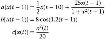
- (a) Choose the model constants: 25, 8, 0.5, and
 as the unknown parameters, reformulate the state estimation problem as a parameter estimation problem with unknown parameter vector,
  and a random walk model with the corresponding process noise variance,
  .
. - (b) Develop the joint UKF algorithm to solve this problem. Run the UKF algorithm and discuss the performance results.
- (c) Develop the joint PF algorithm to solve this problem. Run the PF algorithm and discuss the performance results.
- (d) Choose to “move” the particles using the roughening approach. How do these results compare to the standard bootstrap algorithm?
- (e) Develop the joint linearized (UKF) PF algorithm to solve this problem. Run this PF algorithm and discuss the performance results.
- (a) Choose the model constants: 25, 8, 0.5, and