
Appendix B
Projection Theory
B.1 Projections: Deterministic Spaces
Projection theory plays an important role in subspace identification primarily because subspaces are created by transforming or “projecting” a vector into a lower dimensional space – the subspace [1–3]. We are primarily interested in two projection operators: (i) orthogonal and (ii) oblique or parallel. The orthogonal projection operator “projects” ![]() onto
onto ![]() as
as ![]() or its complement
or its complement ![]() , while the oblique projection operator “projects”
, while the oblique projection operator “projects” ![]() onto
onto ![]() “along”
“along” ![]() as
as ![]() . For instance, orthogonally projecting the vector
. For instance, orthogonally projecting the vector ![]() , we have
, we have ![]() or
or ![]() , while obliquely projecting
, while obliquely projecting ![]() along
along ![]() is
is ![]() .
.
Mathematically, the ![]() ‐dimensional vector space
‐dimensional vector space ![]() can be decomposed into a direct sum of subspaces such that
can be decomposed into a direct sum of subspaces such that
then for the vector ![]() , we have
, we have
with ![]() defined as the projection of
defined as the projection of ![]() onto
onto ![]() , while
, while ![]() defined as the projection of
defined as the projection of ![]() onto
onto ![]() .
.
When a particular projection is termed parallel (![]() ) or “oblique,” the corresponding projection operator that transforms
) or “oblique,” the corresponding projection operator that transforms ![]() onto
onto ![]() along
along ![]() is defined as
is defined as ![]() , then
, then
with ![]() defined as the oblique projection of
defined as the oblique projection of ![]() onto
onto ![]() along
along ![]() , while
, while ![]() defined as the projection of
defined as the projection of ![]() onto
onto ![]() along
along ![]() .
.
When the intersection ![]() , then the direct sum follows as
, then the direct sum follows as
The matrix projection operation (![]() ) is
) is ![]() (
(![]() ) a linear operator in
) a linear operator in ![]() satisfying the properties of linearity and homogeneity. It can be expressed as an idempotent matrix such that
satisfying the properties of linearity and homogeneity. It can be expressed as an idempotent matrix such that ![]() with the null space of
with the null space of ![]() given by
given by ![]() . Here
. Here ![]() is the projection matrix onto
is the projection matrix onto ![]() along
along ![]() iff
iff ![]() is idempotent. That is, the matrix
is idempotent. That is, the matrix ![]() is an orthogonal projection if and only if it is idempotent (
is an orthogonal projection if and only if it is idempotent (![]() ) and symmetric (
) and symmetric (![]() ).
).
Suppose that ![]() '
'![]() , then
, then ![]() with the vectors defined as “mutually orthogonal.” If
with the vectors defined as “mutually orthogonal.” If ![]() '
'![]() , then
, then ![]() is orthogonal to
is orthogonal to ![]() expressed by
expressed by ![]() spanning
spanning ![]() and called the orthogonal complement of
and called the orthogonal complement of ![]() . If the subspaces
. If the subspaces ![]() and
and ![]() are orthogonal
are orthogonal ![]() , then their sum is called the direct sum
, then their sum is called the direct sum ![]() such that
such that
When ![]() and
and ![]() are orthogonal satisfying the direct sum decomposition (above), then
are orthogonal satisfying the direct sum decomposition (above), then ![]() is the orthogonal projection of
is the orthogonal projection of ![]() onto
onto ![]() .
.
B.2 Projections: Random Spaces
If we define the projection operator over a random space, then the random vector (![]() ) resides in a Hilbert space (
) resides in a Hilbert space (![]() ) with finite second‐order moments, that is, 2
) with finite second‐order moments, that is, 2
The projection operator ![]() is now defined in terms of the expectation such that the projection of
is now defined in terms of the expectation such that the projection of ![]() onto
onto ![]() is defined by
is defined by
for ![]() the pseudo‐inverse operator given by
the pseudo‐inverse operator given by ![]() .
.
The corresponding projection onto the orthogonal complement (![]() ) is defined by
) is defined by

Therefore, the space can be decomposed into the projections as
The oblique (parallel) projection operators follow as well for a random space, that is, the oblique projection operator of ![]() onto
onto ![]() along
along ![]()
and therefore, we have the operator decomposition for 2
for ![]() is the oblique (parallel) projection of
is the oblique (parallel) projection of ![]() onto
onto ![]() along
along ![]() and
and ![]() is the oblique projection of
is the oblique projection of ![]() onto
onto ![]() along
along ![]() .
.
B.3 Projection: Operators
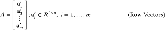
Let ![]() then the row space of
then the row space of ![]() is spanned by the row vectors
is spanned by the row vectors ![]() , while the column space of
, while the column space of ![]() is spanned by the column vectors
is spanned by the column vectors ![]() . That is,
. That is,
and
Any vector ![]() in the row space of
in the row space of ![]() is defined by
is defined by

and similarly for the column space

Therefore, the set of vectors ![]() and
and ![]() provide a set of basis vectors spanning the respective row or column spaces of
provide a set of basis vectors spanning the respective row or column spaces of ![]() and, of course,
and, of course, ![]() .
.
B.3.1 Orthogonal (Perpendicular) Projections
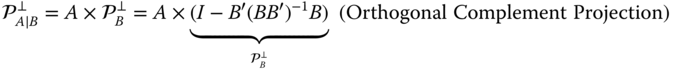
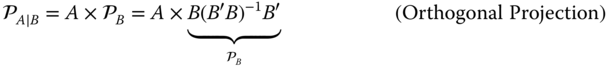
Projections or, more precisely, projection operators are well known from operations on vectors (e.g. the Gram–Schmidt orthogonalization procedure). These operations, evolving from solutions to least‐squares error minimization problem, can be interpreted in terms of matrix operations of their row and column spaces defined above. The orthogonal projection operator (![]() ) is defined in terms of the row space of a matrix
) is defined in terms of the row space of a matrix ![]() by
by
with its corresponding orthogonal complement operator as
These operators when applied to a matrix “project” the row space of a matrix ![]() onto (
onto ( ![]() ) the row space of
) the row space of ![]() such that
such that ![]() given by
given by

and similarly onto the orthogonal complement of ![]() such that
such that
Thus, a matrix can be decomposed in terms of its inherent orthogonal projections as a direct sum as shown in Figure B.1a, that is,
Similar relations exist if the row space of ![]() is projected onto the column space of
is projected onto the column space of ![]() , then it follows that the projection operator in this case is defined by
, then it follows that the projection operator in this case is defined by
along with the corresponding projection given by
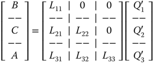
Numerically, these matrix operations are facilitated by the LQ‐decomposition (see Appendix C) as

where the projections are given by

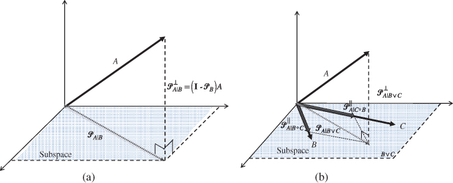
Figure B.1 Orthogonal and oblique projections. (a) Orthogonal projection of  onto
onto  (
( ) and its complement (
 ). (b) Oblique projection of
  onto
onto  along
along  (
( ).
).
B.3.2 Oblique (Parallel) Projections
The oblique projection (![]() ) of the
) of the ![]() onto
onto ![]() along (
along (![]() ) the
) the ![]() is defined by
is defined by ![]() . This projection operation can be expressed as the rows of two nonorthogonal matrices (
. This projection operation can be expressed as the rows of two nonorthogonal matrices (![]() and
and ![]() ) and their corresponding orthogonal complement. Symbolically, the projection of the rows of
) and their corresponding orthogonal complement. Symbolically, the projection of the rows of ![]() onto the joint row space of
onto the joint row space of ![]() and
and ![]() (
(![]() ) can be expressed in terms of two oblique projections and one orthogonal complement. This projection is illustrated in Figure B.1
b, where we see that the
) can be expressed in terms of two oblique projections and one orthogonal complement. This projection is illustrated in Figure B.1
b, where we see that the ![]() is first orthogonally projected onto the joint row space of
is first orthogonally projected onto the joint row space of ![]() and
and ![]() (orthogonal complement) and then decomposed along
(orthogonal complement) and then decomposed along ![]() and
and ![]() individually enabling the extraction of the oblique projection of the
individually enabling the extraction of the oblique projection of the ![]() onto
onto ![]() along (
along (![]() ) the
) the ![]() .
.
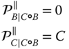
Pragmatically, this relation can be expressed into a more “operational” form that is applied in Section 6.5 to derive the N4SID algorithm 1 ,4, that is,
for ![]() the pseudo‐inverse operation (see Appendix C). Oblique projections also have the following properties that are useful in derivations:
the pseudo‐inverse operation (see Appendix C). Oblique projections also have the following properties that are useful in derivations:
Analogously, the orthogonal complement projection can be expressed in terms of the oblique projection operator as
Numerically, the oblique projection can be computed again using the LQ‐decomposition (see Appendix C).
where the oblique projection of the ![]() onto
onto ![]() along the
along the ![]() is given by
is given by
Some handy relationships between oblique and orthogonal projection matrices are given in Table B.1 (see [1–3, 5] for more details).1
Table B.1 Matrix Projections.
| Projection: operators, projections, numerics | |||
| Operation | Operator | Projection | Numerical (LQ‐decomposition) |
| Orthogonal | |||
| Oblique | |||
| Relations | |||
| — | — | ||
| — | — | ||
| — | |||
| — | |||
References
- 1 van Overschee, P. and De Moor, B. (1996). Subspace Identification for Linear Systems: Theory, Implementation, Applications. Boston, MA: Kluwer Academic Publishers.
- 2 Katayama, T. (2005). Subspace Methods for System Identification. London: Springer.
- 3 Verhaegen, M. and Verdult, V. (2007). Filtering and System Identification: A Least‐Squares Approach. Cambridge: Cambridge University Press.
- 4 Behrens, R. and Scharf, L. (1994). Signal processing applications of oblique projection operators. IEEE Trans. Signal Process. 42 (6): 1413–1424.
- 5 Tangirala, A. (2015). Principles of System Identification: Theory and Practice. Boca Raton, FL: CRC Press.