
Reality Check
The World Is Relational
In today’s enterprise environments, relational databases are the strategic method for data storage. For an enterprise-strength XML, it is crucial to integrate with this technology. This chapter explores paths of migration from and to relational databases as well as concepts of collaboration between the XML format and the relational format.
The chapter starts by giving an introduction into the relational data model and its implementation—SQL. We then compare the features found in SQL (data types and tables) with those offered by XML Schema. We will show how XML schemata can be translated into relational schemata, and vice versa. Finally, we will discuss two commercial implementations (Tamino X-Node and Experanto) that collaborate with relational databases via schema mapping.
11.1 MOTIVATION
Relational databases became a strategic data storage technology when client-server architectures in enterprises emerged. With different clients requiring different views on the same data, the ability to freely construct complex data structures from the simplest data atoms was crucial—a requirement that the classical hierarchical database systems could not fulfill. Relational technology made the enterprise data view possible, with one (big) schema describing the information model of the whole enterprise. Thus, each relational schema defines one ontology, one Universe of Discourse.
And this is the problem. Most enterprises cannot afford to be a data island anymore. Electronic business, company mergers, collaborations such as automated supply chains or virtual enterprises require that information can be exchanged between enterprises and that the cost of conversion is low. This is not the case if conversion happens only on a bilateral level, starting from scratch with every new partner.
XML represents a way to avoid this chaos. Because of its extensibility, XML allows the use of generic, pivot formats for various proprietary company formats. Usually business groups and associations define these formats. If such a format does not satisfy the needs of a specific partner completely, it is relatively easy to remedy by dialecting—extending the generic format with additional specific elements. This is why the integration of XML with relational technology is all important for enterprise scenarios. We will see that XML Schema has been designed very carefully with this goal in mind.
11.2 DATABASES
Logically, relational databases have a very simple structure. The fact that the implementation of a good relational database management system (RDBMS) is not simple at all, and that developers of RDBMSs have invested an incredible amount of work to get decent performance out of this clear and logical concept, is a different story.
When discussing relational databases in context with XML, there are two application areas to keep in mind:
![]() One application is to represent existing data in the RDBMS in XML format. This is important for organizations that store most of their enterprise data in relational form and want to leverage this data for electronic business.
One application is to represent existing data in the RDBMS in XML format. This is important for organizations that store most of their enterprise data in relational form and want to leverage this data for electronic business.
![]() The second is to store existing XML data in relational databases. With mechanisms for referential integrity, transaction logic, backup, and recovery, a database always provides safer storage for data than a simple file system. Of course, it is not always necessary to select an RDBMS for that purpose. Native XML databases can store XML data more efficiently and require less effort when creating an appropriate data model. However, a native XML database is not always at hand, and an RDBMS may provide easier access to the data from existing legacy applications.
The second is to store existing XML data in relational databases. With mechanisms for referential integrity, transaction logic, backup, and recovery, a database always provides safer storage for data than a simple file system. Of course, it is not always necessary to select an RDBMS for that purpose. Native XML databases can store XML data more efficiently and require less effort when creating an appropriate data model. However, a native XML database is not always at hand, and an RDBMS may provide easier access to the data from existing legacy applications.
The Standard Query Language (SQL) is the widely accepted standard for accessing an RDBMS (see Section 11.6. Originally developed to support database table creation, query, update, delete, and insert operations, SQL has been enhanced and expanded over the years and now includes additional means for constraint validation and support of object-oriented databases. SQL-99 goes far beyond the relational data model. However, most RDBMSs don’t support SQL-99, and if they do, they only support a subset. I will therefore restrict the discussion to SQL-92 but give notice where new SQL-99 features solve problems that cannot be solved with SQL-92. Most RDBMSs implement a subset of SQL-92 but enhance it with proprietary extensions. In this discussion, I will stay close to the ANSI or ISO standard.
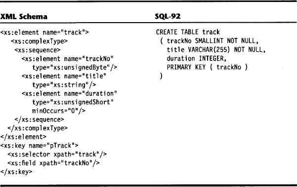
Representing the content of a relational database in XML is relatively easy. The SQL-99 table and type system (and hence the table and type systems of previous SQL editions) is a strict subset of the XML Schema type system. XML Schema looks the way it looks because it was designed to be compatible with SQL-99 (thanks to the intensive participation of DBMS manufacturers). Thus we can easily represent existing relational data with XML Schema without information loss. The opposite way—storing XML data in relational databases without information loss—is not so easy, however.
11.3 THE RELATIONAL DATA MODEL
A relational database basically consists of a set of two-dimensional tables. These tables are organized in unnamed rows and named columns. In relational algebra, tables are called relationships, columns are called attributes, and rows are called tuples. Each row contains a data record, and within such a record, each column represents a data field. Duplicate rows are not allowed. The sequence of rows and columns is not ordered. Two tables have the same type if they have the same set of columns.
Keys are used to identify rows in a table uniquely. Each key consists of one or several fields (columns) chosen in a way that the value or the combined values identify each row uniquely. A key that consists of a minimum number of fields and still satisfies this condition is called a primary key. Foreign keys are field combinations whose combined values can match with primary keys in other tables. This allows us to use tables as relationships: A table that has two foreign keys can relate two other tables to each other. That is the whole idea behind the relational data model: A table represents a relationship.
11.4 THE RELATIONAL ALGEBRA
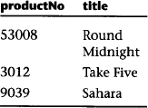
Equally simple is the relational algebra. First, there are set operations:
The operations can be applied to two tables of the same type. The result (shown below) is a table with rows reflecting the union, intersection, and difference between the rows of the original tables.
Table A
| productNo | title |
| 53008 | Round Midnight |
| 3012 | Take Five |
Table B
| productNo | title |
| 9039 | Sahara |
| 53008 | Round Midnight |
Then there are three specific relational operations:
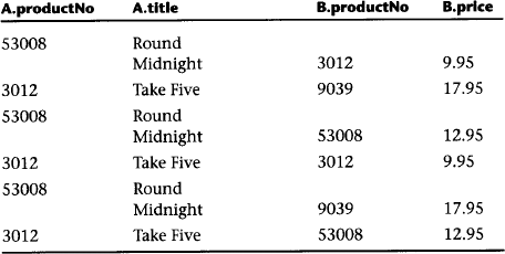
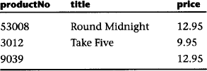
In a Cartesian product, given two tables A and B, the Cartesian product A×B consists of all rows (a1, a2, …, an, b1, b2, …, bn) where (a1, a2,…, an) is a row from A and (b1, b2, …, bn) is a row from B. So, if A has 3 columns and 5 rows, and B has 2 columns and 3 rows, A × B has 5 columns and 15 rows. A smaller example is shown below:
Table A
| productNo | title |
| 53008 | Round Midnight |
| 3012 | Take Five |
Table B
| productNo | price |
| 3012 | 9.95 |
| 9039 | 17.95 |
| 53008 | 12.95 |
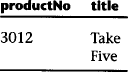
In projection, given a table A, P(A,c1,c2, …, cn) is called a projection of table A on (c1,c2, …, cn) if all columns ai in A that are not specified in (c1,c2, …, cn) are removed from A. Duplicate rows that may have been created in the process are removed, too. For example:
| productNo | title | artist |
| 53008 | Round Midnight | Thelonious Monk |
| 3012 | Take Five | Dave Brubeck |
| artist | title |
| Thelonious Monk | Round Midnight |
| Dave Brubeck | Take Five |
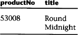
In selection, given a table A and a Boolean function F with arguments from the set of columns {a1, a2, …, an} in A, the selection A: F of table A with selector predicate F consists of all rows from A (and only such rows) satisfying predicate F. For example:
Table A
| productNo | title |
| 53008 | Round Midnight |
| 3012 | Take Five |
| 9039 | Sahara |
| productNo | title |
| 53008 | Round Midnight |
| 9039 | Sahara |
This is all we need. We can now derive two well-known relational operators from the basic operations defined above:
![]() The general join operation A × B: F is nothing but a Cartesian product of two tables A and B followed by a selection with some predicate F.
The general join operation A × B: F is nothing but a Cartesian product of two tables A and B followed by a selection with some predicate F.
![]() In case of the familiar natural join operation A ⇔ B the predicate F consists of a test of one or several column pairs from A and B for equality. Because this results in identical columns, a projection is also performed, to drop duplicate columns. The following example shows a natural join of tables A and B by column productNo:
In case of the familiar natural join operation A ⇔ B the predicate F consists of a test of one or several column pairs from A and B for equality. Because this results in identical columns, a projection is also performed, to drop duplicate columns. The following example shows a natural join of tables A and B by column productNo:
Table A
| productNo | title |
| 53008 | Round Midnight |
| 3012 | Take Five |
Table B
| productNo | price |
| 3012 | 9.95 |
| 9039 | 17.95 |
| 53008 | 12.95 |
| productNo | title | price |
| 53008 | Round Midnight | 12.95 |
| 3012 | Take Five | 9.95 |
One problem with two-dimensional tables is that we must specify all fields in all records. For example, if we have a table person that contains columns for first name, middle name, and last name, then any person record stored in the table must have a first name, middle name, and last name. This is clearly not acceptable, and consequently, relational databases recognize the concept of null values. Any data field in a relational database can contain a “real” value or a null value that means a real value is not known. It is possible to deny the use of null values for certain columns. In particular, columns used for primary keys must not contain null values.
Null values allow the introduction of a new operation: the outer join. The outer join is constructed from the join operation by uniting the rows of the join with the rows of the original tables A and/or B. Because A and B have a different type than the result of the join A×B : F, the rows of A and B are padded with null values before that operation: (a1, a2, …, an, null, null, …, null) and (null, null,…, null, b1, b2, …, bn).
If only the padded rows of table A are added, we speak of a left outer join; if only the padded rows of table B are added, we speak of a right outer join. If both are added, we speak of the full outer join. The following example shows a right outer natural join by column productNo.
Table A
| productNo | title |
| 53008 | Round Midnight |
| 3012 | Take Five |
Table B
| productNo | price |
| 3012 | 9.95 |
| 9039 | 17.95 |
| 53008 | 12.95 |
11.5 NORMALIZATION
The design of relational models requires a sequence of normalization steps. Each step splits the complex data structures of the original model into simpler constructs and reduces redundancies and dependencies between data items. This starts with First Normal Form (1NF), which requires that all column values are atomic. This is in stark contrast to the XML data model with its hierarchy of complex elements.
The relational normalization continues with Second Normal Form (2NF) up to 5NF. These Normal Forms deal more or less with the relationships between column values and keys. In the context of this book they are of no interest; it is the 1NF that causes us some problems.
When registering XML schemata with an XML-enabled relational database, it is the XML access layer of the database that will perform this normalization for us. It will resolve the hierarchical structure of the XML schema into a set of flat SQL tables. To understand this process, we will do this transformation manually.
11.5.1 Defining the Target Format
We will construct a small relational database and demonstrate normalization to First Normal Form. We sidestep a course in SQL for now by constructing our database in the form of an XML document! This has the additional benefit of showing us how relational structures can be implemented in XML.
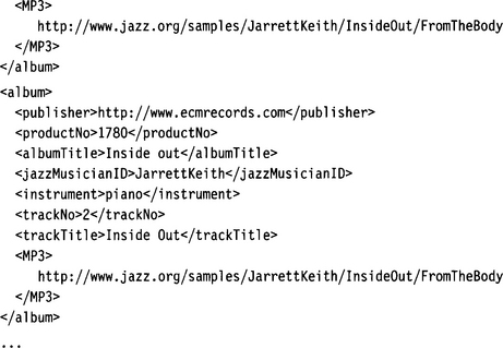
The concept is simple: The root element of our document represents the whole database. The tables are represented as repeating child elements of this root element. The column values are child elements of these elements, that is, grandchildren of the root element. A person table, for example, would look like this:
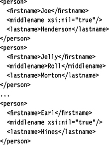
Note that we have used nil values here to represent relational null values. This is just to make the XML layout more similar to the relational layout. As nilvalues can only be used with elements and not with attributes, we always represent table columns with elements.
11.5.2 The Original Schema
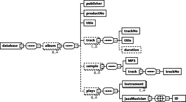
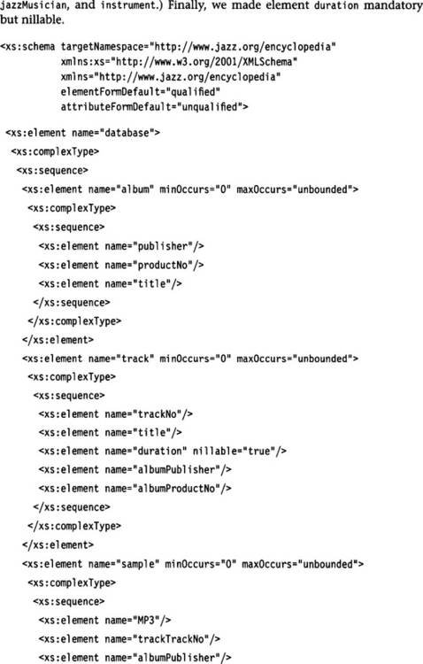
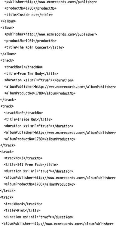
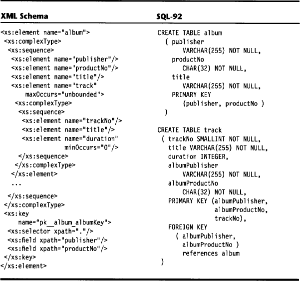
What we are going to do is to normalize our album schema from Chapter 8. We have included all global definitions as local definitions and simplified this schema a bit—at this point we are not interested in data types and annotations. We have also enclosed this album in a root element database. Figure 11.1 shows a diagram of the database.
11.5.3 Steamrolling the Schema
We are now going to convert this table into First Normal Form. Plainly speaking, 1NF means that each table field contains only a leaf element. This is clearly not the case with album. Three child elements (plays, track, sample) of album are repeating elements and, in addition, have a complex structure. They are tables themselves. We therefore remove these child elements from album and make them child elements of database; they become full database tables (see Figure 11.2, page 406).
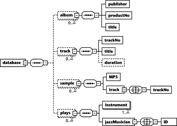
Figure 11.2 Much better, but still not perfect. Note that we made track optional because its former parent node album was optional.
There are still two columns that contain fields with complex structures: jazzMusician and track. This is easy to solve. We can simply collapse jazzMusician and ID into jazzMusicianID; track and trackNo into trackTrackNo.
11.5.4 Introducing Key Relationships
Unfortunately, our effort to flatten the album schema has resulted in a loss of structural information. The tables album, plays, track, and sample are completely uncorrelated. We solve this problem by declaring the combination of publisher and productNo as a primary key for album records, and by introducing elements albumPublisher and al bumProductNo into the tables plays, track, and sample. These fields can then act as foreign keys relating to the album record to which a particular record from plays, track, or sample belongs (see Figure 11.3).
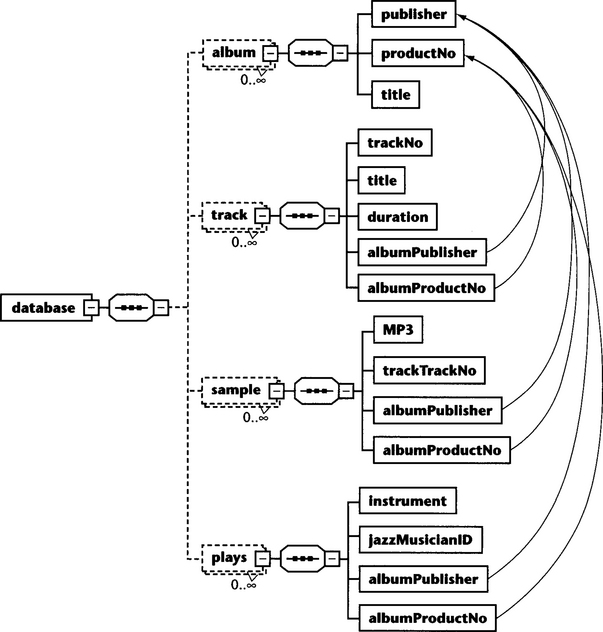
In the following listing, all the primary and secondary keys are defined. All keys are now defined on the database level. Because of this, trackNo as a key for track has become ambiguous—trackNo is only unique in the context of one album element. We have fixed this by adding albumPublisher and albumProductNo to the keys pk_track_trackNo and fk_sampletrack.
We have also removed the maxOccurs=“unbounded” from plays/instrument. Instead of having one plays element with several instrument elements, we will have several plays elements with the same jazzMusician and album but with different instruments. (plays represents a ternary relationship between album, jazzMusician, and instrument.) Finally, we made element duration mandatory but nillable.
11.5.5 Preserving Sequential Order
Although we have now remodeled the parent-child relations of the original schema by introducing primary and foreign keys, we still face some information loss: The cardinality constraints are gone. The constraint that an album must contain at least one track is no longer there! We cannot express this constraint in terms of relational syntax. Relational database systems, however, allow expressing such constraints via Integrity Rules (see Section 11.9.
And there is still another information loss: Repeating elements in XML are ordered. In the original document we would have been able to address the second track element with the XPath expression album/track[2]. In a relational table, in contrast, the rows form an unordered set. There is no guarantee that a query returns the rows in the sequence in which they were inserted. Fortunately, our track table contains a column trackNo. We could use this field to sort returned records when we query the database. If the sequence of the plays and sample records were important, too, we would have to introduce similar numbering fields into these elements.
A document instance of our schema would now look like the following:
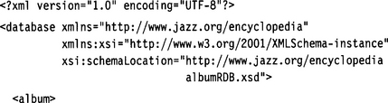
We now have a document with content in relational First Normal Form. The original element album that represented a business object is split into many separate records distributed over various tables.
11.5.6 Recomposing Original Document Nodes
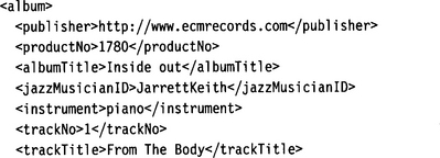
We could apply relational operations on the content to create composite records that combine records from the various tables. To recombine all the tables album, plays, track, and sample we would need to perform the following steps:
1. Compute the natural left outer join between album and plays using the keys pk_album_albumKey and fk_plays_album as a selection constraint. We choose the outer join because albums without plays elements are allowed. In the process, the fields albumPublisher and albumProductNo from table plays are removed.
2. Sort the table track in ascending order using the field trackNo as sort criterion.
3. Compute the natural join between the result from step 1 and the sorted track table from step 2 using the keys pk_album_albumKey and fk_track_album as a selection constraint. We do not use an outer join here because albums require at least one track. In the process, the fields albumPublisher and albumProductNo from table track are removed.
4. Compute the natural left outer join between album and sample using the keys pk_album_albumKey and fk_sample_album as a selection constraint. We choose the outer join because albums without sample elements are allowed. In the process, the fields albumPublisher and albumProductNo from table sample are removed.
5. Finally, we have to consider the relationship between sample and track. We throw out all records for which the selection constraint given by the keys pk_tracktrackNo and fk_sample_track does not hold. After this operation, the column sample/trackTrackNo has become redundant. We perform a projection to remove this column.
6. We have a name clash. Both album and track contain a column named title. We rename these elements albumTitle and trackTitle.
The above operations result in a set of records that looks like the following:
For every valid combination of album, plays, track, and sample we get a new record. What we do not get with pure relational operations is the nice tree structure of the original document, although SQL provides some means for aggregation in queries (see next section). This is left to application logic, either expressed in some programming language or by means of SQL-99 [Krishnamurthy2000].
11.6 BRIEF INTRODUCTION TO SQL
This section gives a brief introduction to SQL-92 and then discusses how SQL-99 extends SQL-92. Note that this section is intended to give an overview about the features of SQL, not to provide an in-depth tutorial. Interested readers may refer to the many excellent textbooks about this topic, such as [Silberschatz 2001]. Although implementations of SQL-99 are scarce and incomplete, it is important because the type and structural system of XML Schema was designed as a superset of the type and structural system of SQL-99.
11.6.1 Queries
The query part of SQL is based on relational algebra with certain modifications and enhancements. A typical SQL query looks like
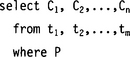
with C1, C2,…,Cn being column names, t1, t2,…,tm being table names, and P a predicate. If a column name does not uniquely identify a column, it must be prefixed with the table name, using the familiar dot notation. This query is equivalent to the following relational operations:
1. Constructing a Cartesian product from t1, t2,…, tm. This is specified in the from clause by listing the participating tables.
The from clause may also specify a join. This is done by specifying the join type (inner join, left outer join, right outer join, full outer join), the join predicate (natural, on predicate), and which columns of the join are used (using C1, C2,…,Cn); for example:
![]()
2. Applying a selection with predicate P. This is done in the where clause. The where clause allows comparisons between columns and/or constants. Comparisons between arithmetic expressions and between string expressions are possible, too. These comparisons can be combined in a Boolean expression with the operators and, or, and not.
3. Projecting the result onto columns C1, C2,…,Cn. This is specified in the select clause. Alternatively, the select clause may specify an asterisk (*) to denote all columns, meaning to skip this step.
In contrast to pure relational theory, SQL allows duplicates in tables and query results. The keyword distinct can be specified after select to remove duplicates; the keyword all, to keep duplicates.
The select clause can be used to apply arithmetic operations (+,−,*,/) on column names, provided these columns have a numeric type; for example:
![]()
Aggregating functions such as avg(), min(), max(), sum(), and count() are used to compute the average, minimum, maximum, sum, and number of rows over columns.
A variety of string operations (concatenation, substring, conversion from upper- to lowercase and vice versa, etc.) are also available.
The select clause can be used to rename the columns of the query result using the keyword as. For example,
![]()
renames the columns C1, C2,…,Cn to R1, R2,…,Rn.
There are a few optional clauses that can be specified after the where clause:
![]() Sorting the result is possible by specifying the clause
Sorting the result is possible by specifying the clause
![]()
with Ci, Cj specifying the sort fields. The keywords asc or desc may be appended to specify ascending or descending order.
![]() Aggregation of query results is possible with the clause
Aggregation of query results is possible with the clause
![]()
This will result in a single result record for each combination of Ck and C1. The select clause must cumulate all columns that are not specified in the group by clause but are specified in the select clause with aggregating functions such as sum() or avg().
It is possible to apply additional predicates on the results of the group by clause to select only certain rows from the result set obtained by group by. This is done with the clause having Q where Q is a selection predicate.
Select statements can be nested—that is, the result of a query can be used as an input table for another query. The where clause provides several operators to relate to such result sets. For example,
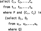
tests whether the value tuple (Ci, Cj) is found in the result set of the nested query. Similarly, it is possible to test whether a given value is greater or smaller than all or some of the values returned by the nested query.
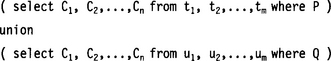
Query results can be combined with set operations such as union, intersection, and difference. This is done with the operators union, intersect, and except. A condition is that both operands of such an operation have an identical column schema:
Although there is more to know about SQL queries, this should be sufficient for a brief introduction. In addition to queries, SQL provides commands for table creation, for inserting, updating, and deleting table rows, and for administration.
11.6.2 Table Creation
Tables are created with the create command:
C1, C2,…,Cn define the column names, and D1, D2,…,Dn define the data types of each column (see Section 11.7. Each of the Ci Di pairs can be postfixed with not null to indicate that no null values are allowed in this column.
Other integrity constraints are
![]()
to define a primary key consisting of the columns Ci, Cj,… (similar to the key clause in XML Schema),
![]()
to define a foreign key consisting of the columns Ci, Cj,… (similar to the keyref clause in XML Schema) and referring to table t, and
![]()
with P being a predicate over the columns C1, C2,…,Cn. This predicate is checked whenever a new row is inserted or a row is updated.
The command alter table is used to modify existing tables (adding or removing of columns), and the command drop table is used to remove tables from a schema.
11.6.3 Table Modification
Rows can be deleted from a table with the del ete command:
![]()
The from clause specifies the table, the where clause (see Section 11.6.1) specifies a predicate P, which selects the rows to be deleted.
New rows can be created with the insert command:
![]()
The into clause specifies the table; the values clause specifies a value for each column. As rows in a table form an unordered set, it is not necessary to specify where to insert the new row.
Existing rows can be modified with the update command:
![]()
The set clause specifies which columns should be modified. The expressions Ei, Ej are the new values and can consist of constants, or arithmetic or string algebraic expressions computing a new value. These expressions can refer to existing column values. The where clause (see Section 11.6.1) specifies a predicate P, which selects the rows to be modified.
Multiple update, insert, and delete operations can be combined in transactions. The end of a transaction (and the beginning of the next) is defined with the commands commit work or rollback work.
11.6.4 Views
The ability to create views on a schema is an important facility of SQL. Views are typically used to give users restricted access to the tables of a schema. This allows decentralized maintenance of a data pool: In a large corporation, individual aspects of a table can be maintained by different departments without the need to perform each update through a central administration. For example, if we have a table customer, the sales department can be responsible for the sales contacts and sales history of a customer, the accounting department can be responsible for the customers’ accounts, and so forth.
In SQL a view is created with the create view command:
![]()
Q can be any legal query expression, including query expressions across multiple tables and on aggregations. The created view v can then be used in the from clause of a query instead of a table.
Updates on views are possible, too, but they are restricted on views that are defined by simple query expressions. Most implementations, for example, do not support updates on views that are defined with query expressions containing aggregates (group by).
Views can be defined across multiple tables by utilizing SQL’s join facilities. Such a view can represent a set of multiple tables as a single virtual table to the user.
11.6.5 SQL-99
SQL-99 introduces object-orientation into relational databases. By doing so, it departs from pure relational theory; consequently, the approach of SQL-99 is called object-relational. Nevertheless, SQL-99 maintains backward compatibility with earlier versions of SQL. The most important change is that SQL-99 allows non-atomic, structured table columns (also called nested tables). In particular, SQL-99 introduces built-in constructors such as row and array. It is also possible to define your own structured data types:
![]()
C1, C2,…,Cn define the column names, and D1, D2,…,Dn define the data types of each column, including other structured types and collections. These data types can be used everywhere types are specified, including the create table command.
We can access the components of such a structured type by using the familiar dot notation, for example, customer.name.first. User-defined types cannot be used directly in arithmetic expressions and comparisons; instead the user must provide appropriate access methods. Such methods are declared in the create type command:
But they must be implemented in a separate clause:
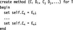
Ek, …, En are expressions derived from the parameters Ci, Cj,… The table columns are addressed via self.Ck, …, self.Cn.
SQL-99 allows the construction of type hierarchies. The expression
![]()
establishes an inheritance relationship where T1 inherits columns and methods from T2.
Tables can be derived from a type,
![]()
with t specifying the table name and T the name of a defined type. The table t is created with a column for each property of type T. The table also inherits the methods of T. In terms of object-oriented programming, each row in table t is now an instance of type T. Because these rows are regarded as objects, an objectidentifier is generated for each row. These object identifiers can be used to refer to these rows. It is possible to store such identifiers in other tables: Their data type is ref (t), with t identifying the table that is referred to. This reference data type allows the new pointer notation in queries:
![]()
Given that Ci is a column of type ref (t2), this expression results in column t2.Ck with the rows identified by the object identifiers stored in t1.Ci.
Of course, there is much more to SQL-99. Its features would surely fill a book of its own.
11.7 SIMPLE DATA TYPES
For the description of SQL data types, I refer to the current working draft for SQL 200x (SQL-4) [Melton2001]. Earlier SQL standards (SQL-99, SQL-92, etc.) and existing implementations differ in some points from this description. However, this working draft is currently the best reference point for comparing XML Schema data types with SQL data types. The mapping between XML Schema data types and SQL data types is described in detail in [Melton2001a] and [Eisenberg2002].
11.7.1 String Data Types
The primitive data type string as defined in XML Schema is based on the Unicode character set (independent of the actual encoding!) and is of unlimited length. In SQL there are several corresponding character string types: CHARACTER, CHARACTER VARYING, CHARACTER LARGE OBJECT (CLOB). (There are also other spellings, such as CHAR and VARCHAR, which are used in earlier SQL editions.) CLOBs are restricted in certain aspects: They cannot be used in primary or foreign keys or unique column combinations.
All character string types are based on character sets supported by SQL. SQL supports various character sets, including ASCII and Unicode. This may require that XML strings be mapped to SQL strings and vice versa. This mapping is implementation defined. In addition, SQL string data types have a fixed or maximum length. The data type CHARACTER has a fixed, schema-defined length (the maximum length is implementation defined, varying between 255 and 4,000 in implementations), while the data type CHARACTER VARYING supports strings of variable length. Again, the maximum length is implementation defined. The CHARACTER LARGE OBJECT typically supports string lengths of up to 2GB. In XML, these data types can be modeled by restricting the string data type with the constraining facets length or maxLength.
In SQL, there are no equivalent standard data types for XML Schema data types derived from string, such as normal izedString or token.
11.7.2 Binary Data Types
Since XML is text based, it does not support binary data in native format. Instead, XML Schema offers two encoded binary formats: hexBinary and base64Binary. Both formats support binary data of unlimited length.
SQL supports the binary data type BINARY LARGE OBJECT that supports large strings of binary data. (Earlier SQL standards also recognize BIT and BIT VARYING.)
11.7.3 The Boolean Data Type
XML Schema supports Boolean values with the data type boolean. SQL supports Boolean values with data type BOOLEAN.
11.7.4 Exact Numeric Types
The only primitive exact numeric data type in XML Schema is decimal. All other exact data types such as integer, long, int, short, and so on, are derived from this data type by restriction. XML Schema does not restrict the upper and lower bound of decimal but requires processors to support at least 18 decimal digits. The SQL data type DECIMAL is almost equivalent to the decimal data type in XML Schema. The maximum number of decimal digits is implementation defined, ranging from 18 to 38 decimal digits.
There is no direct equivalent for the XML Schema integer data type in SQL. However, this data type can be represented in SQL by data type DECIMAL with no fractional digits. For the following integer data types there is a direct equivalence:
| XML | SQL | Range |
| long | BIGINT– | 9,223,372,036,854,775,808 9,223,372,036,854,775,807 |
| int | INTEGER | –2,147,483,648 2,147,483,647 |
| short | SMALLINT | –32,768 32,767 |
11.7.5 Approximate Numeric Types
XML Schema supports the approximate numeric types float and double for single and double precision floating-point numbers according to IEEE 754-1985. With these data types we find the highest compatibility between SQL and OO languages, as IEEE 754-1985 has been adopted by SQL-92 and practically all OO languages. However, the naming can be confusing:
| XML | SQL | Precision |
| float | REAL | 32 bit |
| double | FLOAT | 64 bit |
The SQL data type DOUBLE PRECISION (128 bit) does not have an equivalent in XML Schema.
11.7.6 Date and Time
XML Schema provides a rich set of date and time data types based on ISO 8601. dateTime specifies a precise instant in time (a combination of date and time), date specifies a Gregorian calendar date, and time specifies a time of day. All three types can be specified with or without a time zone. The data type duration specifies an interval in years, months, days, hours, minutes, and seconds, and allows negative intervals, too.
SQL supports date and time values with the data types TIME, DATE, and TIMESTAMP. While both TIME and TIMESTAMP can be specified with or without a time zone, DATE can only be specified without a time zone. (Note: The ODBC database interface does not support TIME and TIMESTAMP with time zone.) TIME and TIMESTAMP support fractions of seconds. The resolution is implementation dependent.
SQL provides a data type INTERVAL with features similar to the XML Schema data type duration. However, not many DBMSs implement this data type.
11.7.7 Other Data Types
XML Schema supports URIs with the data type anyURI. SQL does not have an equivalent to anyURI. However, URIs can easily be stored in CHARACTER VARYING fields.
The QName data type in XML Schema specifies qualified names. It consists of a local part and a namespace part. It is relatively easy to represent such a qualified name in SQL: It is simply mapped to a tuple consisting of a namespace URI and the local name (both stored in CHARACTER VARYING columns). Note that it would be wrong just to store a qualified name as a local name with a prefix! The mapping between prefix and namespace may change at any time.
11.7.8 Type Restrictions
XML Schema provides a rich set of constraining facets to derive user-defined simple data types from built-in data types. SQL allows parameterizing built-in types but in a limited way. For example, it is possible to control the length of a CHARACTER column, or to control the number of decimal and fractional digits in a DECIMAL column. Other parameters such as the constraining facets minInclusive or maxExclusive in XML Schema do not exist in the SQL type system. However, SQL offers other ways to constrain the value of a column (see Section 11.9.
11.7.9 Type Extensions
Restriction is not the only way in XML Schema to derive user-defined types. Type extensions such as type union and extension by list are possible, too. SQL-92 has no equivalent construct. If such types must be mapped onto relational types, the only choice is to store values of these types in their lexical representation, that is, to use the type CHARACTER VARYING or CLOB in SQL. In contrast, SQL-99 allows representing list extensions by defining an ARRAY. A LIST collection type is planned for future versions.
11.7.10 Null Values
All SQL data types support the notion of null values. XML Schema allows nill values for elements but not for attributes (see Section 5.3.16).
11.8 COMPLEX TYPES
Section 11.5 already showed a few examples of how complex types can be mapped onto relational structures. We have seen that relational fields that may either contain a value or null can represent optional elements. We have also seen that repeating elements almost always result in a separate table. Each record in this table contains a foreign key referring to the primary key of the former parent element.
This section discusses how to express hierarchy in relational terms, and how to implement the three basic regular expression operators (sequence, choice, recursion) with the relational methods of SQL-92.
11.8.1 Hierarchy
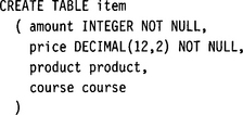
Leaf elements (elements that do not contain child elements) of a cardinality <= 1 and attributes can be implemented as simple table columns (see Table 11.1). Complex elements and leaf elements with cardinality > 1, however, must be implemented as tables. Equipping the parent with a primary key and the child with a foreign key referring to this primary key can preserve parent-child relationships.
Table 11.1
Translating leaf elements into a relational schema. Note that we have to constrain the maximum length of string values, as SQL requires specifying a maximum length for VARCHAR.
Take for example the track element in the example in Section 11.5. Element track is a complex child element of album. Because it is complex, we have to implement it as a separate table. We introduce two fields albumPublisher and albumProductNo to form a foreign key. This key refers to the primary key defined for table album, which consists of the fields publisher and productNo (see Table 11.2).
Because track is defined as a repeating element in album, we also add the fields albumPublisher and albumProductNo to the primary key of track. Otherwise the key would not be unique, as trackNo is only unique within the context of one album instance.
In some cases, however, the creation of a separate table for a complex element can be overkill. Take for example a complex element such as name (first,middle?, last). In such cases we are better off resolving this element into three leaf elements, such as name_first, name_middle?, name_last.
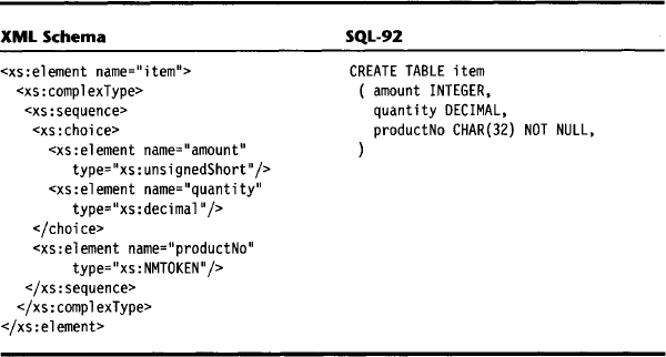
As mentioned above, SQL-99 solves this problem by introducing user-defined structured types. It would be possible to define a structured type for name(first,middle?, last),
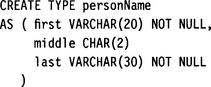
and then use it in a column definition:
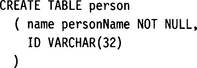
The subfields of a type can be accessed via a dot notation, such as
![]()
11.8.2 Sequence
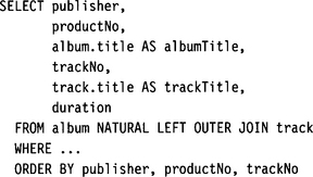
Again, as far as leaf elements are concerned, sequence is easy to establish. A sequence of leaf elements is simply translated into a sequence of table columns. However, for complex elements we lose this sequence information when the complex element forms a table. If the sequence of complex child elements is essential, we must make sure in later queries that the various tables are joined in the right sequence. The SQL query
![]()
joins the two tables album and track in the correct order. The * notation after the SELECT stands for “all fields.” In this case, where more than one table is specified after the FROM keyword, it delivers the Cartesian product.
In our case, however, it would be better to perform an explicit projection. There are three reasons for this: First, we were just lucky that the album schema specified all leaf elements in front of the complex element track. If, for example, the element title followed the element track, the query shown above would deliver the wrong result. Second, we need to rename a column because both album and track contain a title column. Third, we would like to remove the duplicate columns publisher/albumPublisher and productNo/albumProductNo.
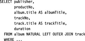
The AS clause is used to rename a column.
For repeating elements (which form their own table), sequence information is lost, too. Rows in relational databases form an unordered set. To maintain the sequence information between the element occurrences, we must equip each of the table rows with a field that numbers the rows in the original sequence, such as trackNo in the table track. Later queries can then use the ORDER BY operation to reestablish the original sequence.
11.8.3 Choice
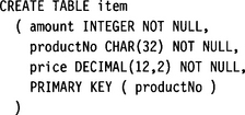
A construct such as the choice connector does not exist in relational schemata. If the choice connector combines two leaf elements, the implementation is relatively easy: Both elements become fields in the table. In each row, one of the fields must have a value and the other must be null (see Table 11.3).
Table 11.3
Translating leaf element choices into a relational schema. Note that one of the columns amount or quantity must be null.
For complex elements combined by a choice connector, the situation is tricky. Both elements are implemented as a table that points via a foreign key to the parent table. If we want to reconstruct the document instances in a query, we must compute the union of two subqueries: The first subquery joins the parent table with the left child table; the second subquery joins the parent table with the right child table. However, unions are only possible when both operands have the same structure. This can sometimes require some ingenuity. The general solution is to cast all noncompatible fields of each operand into a character string and then concatenate these fields into a single character string. This allows a successful union of both subqueries.
Let’s assume the following table structure:
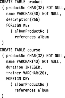
Now let’s assume that an item is the parent of either a product or a course. Product and course have a different layout, so a direct union is impossible. The following SQL query solves the problem:
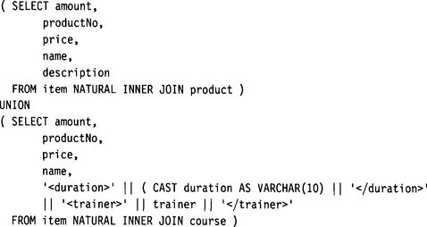
In the second SELECT clause we use string concatenation to combine duration and trainer into a single character string. This string is type compatible with description, so the UNION operator can succeed.
In SQL-99 the problem of alternative complex types is much simpler to solve. Both product and course can be defined as structured types. Table items would simply contain two additional columns product and course, where either one or the other is null. Querying this table would require neither a join nor a union.
11.8.4 Recursion
Recursion is relatively easy to model. The recursive element is implemented as a table. This table has a primary key and a foreign key, with the foreign key referring to this primary key (see Table 11.4).
11.9 CONSTRAINTS
SQL defines a rich arsenal for validating the integrity of relational data:
![]() Domain constraints are the most elementary form of integrity constraints. Domain constraints are used to constrain the value of a single column. They are used to test values inserted into the database and to test queries to make sure that a comparison is valid. Domain constraints resemble the constraining facets for simple types in XML Schema but have more expressive power. For example, a domain constraint can contain a subquery, thus allowing the implementation of cross-field constraints.
Domain constraints are the most elementary form of integrity constraints. Domain constraints are used to constrain the value of a single column. They are used to test values inserted into the database and to test queries to make sure that a comparison is valid. Domain constraints resemble the constraining facets for simple types in XML Schema but have more expressive power. For example, a domain constraint can contain a subquery, thus allowing the implementation of cross-field constraints.
SQL-99 introduces a SIMILAR predicate to test whether strings conform to regular expression syntax. This is comparable to the pattern facet in XML Schema, which constrains the lexical space of a data type to conform to the specified regular expression syntax. Consequently, the predicate SIMILAR can be used to mimic this constraining facet.
![]() Referential integrity constraints are used to declare columns or combinations of columns as unique, as a primary key, or as a foreign key. This functionality is practically equivalent to the unique, key, and keyref constructs in XML Schema. These constraints are applied when records are inserted, updated, or deleted. Operations that would violate these constraints are rejected.
Referential integrity constraints are used to declare columns or combinations of columns as unique, as a primary key, or as a foreign key. This functionality is practically equivalent to the unique, key, and keyref constructs in XML Schema. These constraints are applied when records are inserted, updated, or deleted. Operations that would violate these constraints are rejected.
![]() Cascading actions allow the DBMS to automatically maintain referential integrity by propagating operations such as DELETE or UPDATE along referential chains. For example, in our small database in Section 7.2.4, we established primary/foreign key relations from the tables plays, track, and sample to table album. If we deleted an album record, a cascading delete operation would also delete all records from plays, track, and sample that referred to this specific album record.
Cascading actions allow the DBMS to automatically maintain referential integrity by propagating operations such as DELETE or UPDATE along referential chains. For example, in our small database in Section 7.2.4, we established primary/foreign key relations from the tables plays, track, and sample to table album. If we deleted an album record, a cascading delete operation would also delete all records from plays, track, and sample that referred to this specific album record.
![]() General assertions are constraints that the database must always satisfy. An assertion defines a general query with a Boolean result. This query is executed with each operation that is performed on a table for which the assertion is defined. If the query fails, the operation is rejected. Since general assertions can contain complex queries, they can cause considerable overhead. There is no equivalent construct in XML Schema, but when storing XML documents in a relational database, general assertions can be used to maintain the structural integrity of the document instances.
General assertions are constraints that the database must always satisfy. An assertion defines a general query with a Boolean result. This query is executed with each operation that is performed on a table for which the assertion is defined. If the query fails, the operation is rejected. Since general assertions can contain complex queries, they can cause considerable overhead. There is no equivalent construct in XML Schema, but when storing XML documents in a relational database, general assertions can be used to maintain the structural integrity of the document instances.
![]() Triggers consist of SQL statements that are executed automatically by the DBMS as a side effect of database operations. Triggers contain a criterion that specifies under which conditions the specified statements are executed. Triggers are not defined in SQL-92, but many database implementations support them. SQL-99 defines a standardized model for triggers.
Triggers consist of SQL statements that are executed automatically by the DBMS as a side effect of database operations. Triggers contain a criterion that specifies under which conditions the specified statements are executed. Triggers are not defined in SQL-92, but many database implementations support them. SQL-99 defines a standardized model for triggers.
As you can see, the support for constraints in SQL far surpasses the possibilities provided by XML Schema. However, not every mechanism defined in the standard is implemented in existing DBMSs. For example, Oracle 9i does not support general assertions but supports triggers.
11.10 FROM RELATIONAL TABLES TO XML SCHEMA
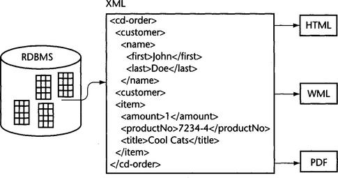
Translating relational data into XML is a frequent operation. Especially when legacy enterprise data must be put on the Web, XML is the format of choice because XML is ideally suited to act as a pivot format from which many other web formats can be generated (Figure 11.4, page 432). The relational data is first translated into a presentation-neutral XML format, which can then be transformed into the target formats.
Constructing an XML schema from a relational table definition is simple and straightforward. The table is converted into an XML element; the sequence of table columns is converted into a sequence of child elements. Mapping SQL data types to simple XML Schema data types is also not a problem (see Section 11.6. Primary keys are converted into key clauses; foreign keys are converted into keyref clauses. Unique constraints are converted into unique clauses. Also, some suitable domain constraints may be represented by user-defined simple data types obtained by applying the appropriate constraining facets to built-in XML Schema data types.
However, with this technique, we only arrive at flat normalized XML schemata, similar to the one obtained in Section 11.5. To construct a deeply nested, treelike XML data structure from a relational schema requires a different approach:
![]() If we are still in possession of the conceptual model that served as a basis for the relational implementation, we can use this conceptual model to create the XML schemata. We can then map the elements of the relational schema onto the elements of the XML schema.
If we are still in possession of the conceptual model that served as a basis for the relational implementation, we can use this conceptual model to create the XML schemata. We can then map the elements of the relational schema onto the elements of the XML schema.
![]() If we are only in possession of the relational schema, a serious reengineering effort is required.
If we are only in possession of the relational schema, a serious reengineering effort is required.
In the first step we re-create the conceptual model (see Chapters 2 and 3). Each table is remodeled as an asset; the table columns become properties. Foreign/primary key relations are translated into an arc originating from the asset to which the primary key belongs. The cardinality constraint of all arcs is “*” (no cardinality constraint).
However, this model is not really complete. We are unable to learn from the relational schema which columns and which key relationships represent alternatives. In many cases, it will be impossible to find out if two fields or two child tables are mutually exclusive. In some cases, however, this knowledge may be hidden in SQL constraints and SQL queries.
In the second step we determine Level 2 Structures, and in the third step we translate the conceptual model into XML Schema (see Chapter 8).
11.11 MEDIATION BETWEEN RDBMS AND XML DATABASES
In this section we introduce two commercial products, Tamino X-Node and Experanto, that can mediate between relational data structures and XML.
11.11.1 Tamino X Node
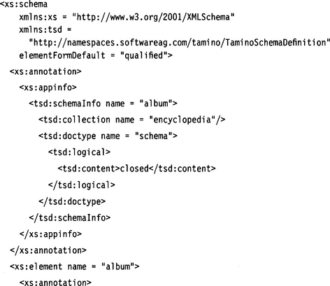
Software AG’s (www.softwareag.com) Tamino XML Server is one of the leading native XML databases. Tamino is able to handle generic (schema-less) XML documents, but for the most efficient operation it requires the definition of schemata where it uses a subset of XML Schema. Document instances can be validated against the schema.
In addition, a Tamino schema describes physical properties—for example, which document nodes should be used to index the document, and in which form. These additional definitions are included in appinfo sections in the schema file. These appinfo sections can also contain information about the storage location of each node—as native XML data within the Tamino data storage, or as relational data. Via its X-Node component, Tamino can access connected (and possibly remote) RDBMSs. Since the storage location can differ from document node to document node, Tamino can compose virtual XML documents from data stored in its own data storage, in relational databases, or other data sources. This not only works for retrieval but also for update, store, and delete operations. The following gives an overview of how the mapping between XML nodes and relational tables and columns is described within the schema’s appinfo sections.
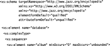
Let’s assume that we store information about jazz albums in a relational database. The following tables are defined:
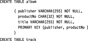
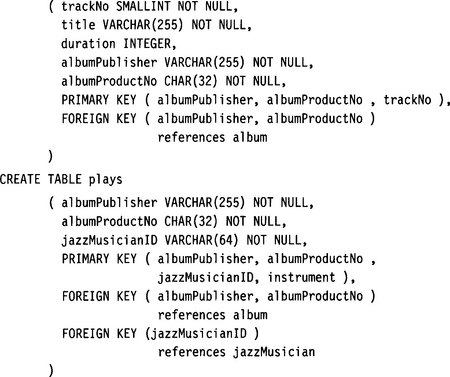
We want to map these SQL schemata to an XML schema similar to the album schema in Chapter 8. In the process, we want to extend the schema and add a sample node. The resulting XML Schema could look like the following:
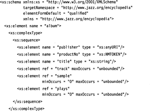
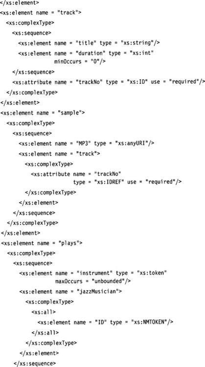
Note that the duration element has type xs:int instead of xs:duration. This was derived from the SQL tables where duration was defined as INTEGER. Most SQL databases do not support the SQL data type INTERVAL. We have also added the definition for element sample and have established a cross-reference between sample and track.
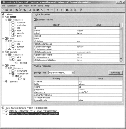
We can now use this schema as input for Tamino’s Schema editor, as shown in Figure 11.5. This editor allows us to map the schema nodes to physical resources such as SQL tables and columns. Basically, each complex element such as track and plays is mapped to the corresponding SQL table. The leaf elements and attributes, in contrast, are mapped to columns of those tables. The exceptions are the element sample and its child elements. These elements are mapped to native fields within Tamino. The consequence is that album instance documents reside in part within Tamino and in part in the connected ODBC database. Nevertheless, it is possible to execute complex queries and to perform update operations (which are carried forward to the connected ODBC database).
Let’s take a closer look at how the definition of the album node looks now:
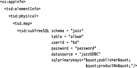
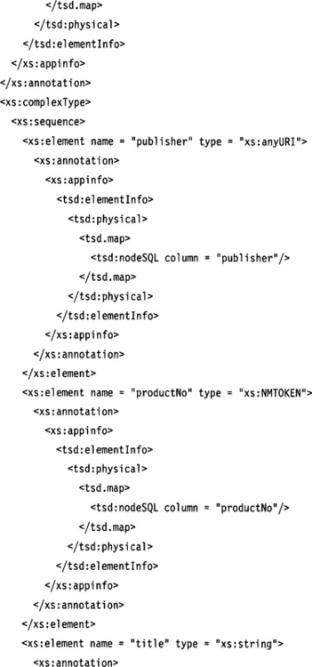
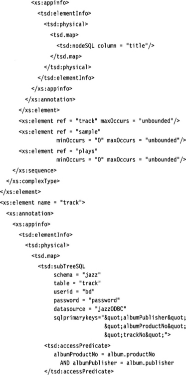
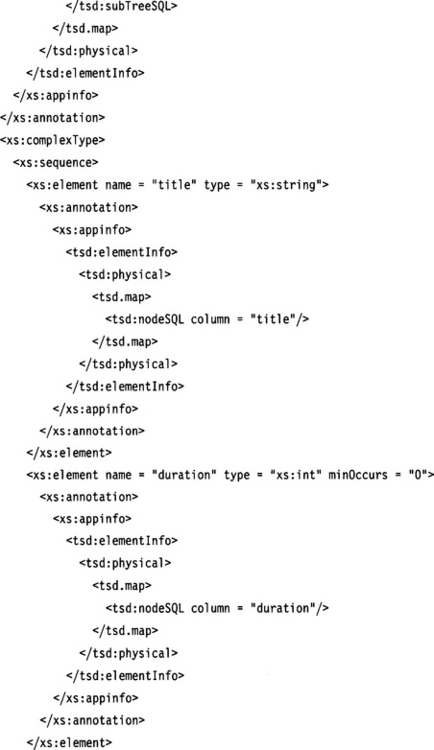
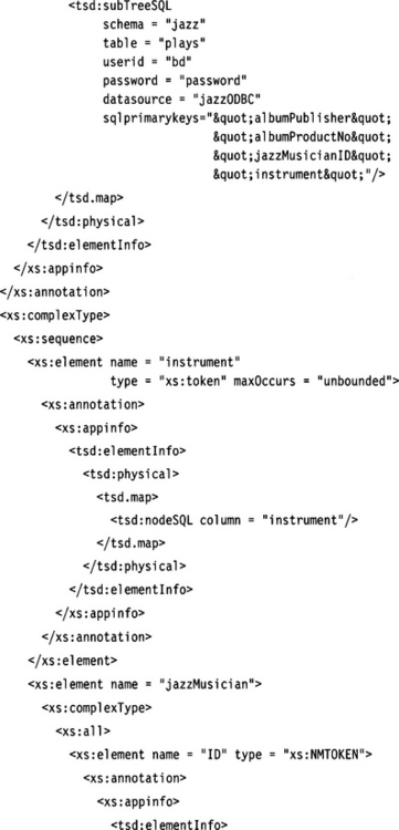
We can see that mappings to SQL tables used for complex elements are described with a tsd:subTreeSQL element. Specified in its attributes are the name of the SQL schema (the name of the database), the name of the table, user ID, and password to allow Tamino to access these tables, and the name of the ODBC data source through which this table is accessed. This setup would allow us to combine various tables from different data sources into one XML document.
The attribute sqlprimarykeys specifies the primary key fields of the specified table. For element track, the additional clause
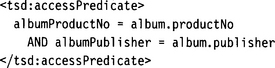
specifies a join criterion to match records from table track to records of table album. The content of the accessPredicate clause will appear in the SQL WHERE clause generated by the Tamino X-Node.
For leaf elements and attributes, the mapping is simpler: We only have to specify the column of the SQL table that has been specified in the ancestor of the respective XML element or attribute. Take for example the element plays/jazzMusician/ID. We have specified column jazzMusicianID. Because the nearest ancestor with a table specification is the element plays and the table specified there is the SQL table plays, we refer to column jazzMusicianID in table plays.
11.11.2 Experanto
Another mediator software between relational databases and the XML world is IBM’s Experanto (formerly XTABLES), which allows transparent access to RDBMSs and other data sources such as web services. Experanto features a completely different architecture from Tamino’s. The core of the system is a powerful XQuery engine.
XQuery 1.0 is currently a W3C Working Draft [Boag2002]. XQuery builds heavily on XPath 2.0 and offers functionality similar to XSLT, but uses an SQL-like syntax to formulate queries. One of its strengths is that it is possible to define functions in XQuery, and XQuery functions may be used recursively as targets of new queries. An XQuery function thus defines a particular view of the information base.
Experanto exploits this feature of XQuery. For relational tables declared to the system, Experanto automatically generates a default view—an XQuery function that can retrieve a raw table record in XML format. Users can define custom views and queries on the basis of this default view. Because XQuery allows joining data sources, views across multiple tables can be defined.
Experanto is basically a schema-less system: The (virtual) document types are constructed by defining XQuery expressions, not by defining schemata using a common schema language. When a schema is needed for the virtual document type—for example, to serve as input to binding generators such as Sun’s JAXB, Enhydra’s Zeus, or Breeze XML Studio (see Section 10.1—the author must create an additional explicit schema. In Section 13.1 we will discuss the problems of view definition in more detail.
Because XQuery—as the name says—is purely a solution for querying XML data sources, and not for their modification, Experanto can only query the connected data sources, but not update them.