13

Domain-Specific Computer Architectures

This chapter brings together the topics discussed in previous chapters as we examine a variety of computer system architectures designed to meet unique user requirements. We will gain an understanding of the user-level requirements and performance capabilities associated with several categories of real-world computer systems.

This chapter will cover the following topics:

• Architecting computer systems to meet unique requirements
• Smartphone architecture
• Personal computer architecture
• Warehouse-scale computing architecture
• Neural networks and machine learning architectures

After completing this chapter, you will understand the decision process used in defining computer architectures to support specific needs. You will have learned the key requirements driving the architectural designs of mobile devices, personal computers, cloud server systems, and neural networks and other machine learning architectures.

Technical requirements

The files for this chapter, including answers to the exercises, are available at https://github.com/PacktPublishing/Modern-Computer-Architecture-and-Organization-Second-Edition.

Architecting computer systems to meet unique requirements

Every device containing a digital processor is designed to perform a particular function or collection of functions. This includes general-purpose devices such as personal computers. A comprehensive list of the required and desired features and capabilities for a particular device or computer system provides the raw information to begin designing the architecture of its digital components.

The list that follows identifies some of the considerations a computer architect must weigh in the process of organizing the design of a digital system:

• The types of processing required: Does the device need to process audio, video, or other analog information? Is a high-resolution graphics display included in the design? Will extensive floating-point or integer mathematics be required? Will the system support multiple, simultaneously running applications? Are special algorithms, such as neural network processing, going to be used?
• Memory and storage requirements: How much RAM will the operating system and anticipated user applications need to perform as intended? How much non-volatile storage will be required?
• Hard or soft real-time processing: Is a real-time response to inputs within a time limit mandatory? If real-time performance is not absolutely required, are there desired response times that must be met most, but not necessarily all, of the time?
• Connectivity requirements: What kinds of wired connections, such as Ethernet and USB, does the device need to support? How many physical ports for each type of connection are required? What types of wireless connections (cellular network, Wi-Fi, Bluetooth, NFC, GPS, and so on) are needed?
• Power consumption: Is the device battery-powered? If so, what is the tolerable level of power consumption for digital system components during periods of high usage, as well as during idle periods? If the system runs on externally provided power, is it more important for it to have high processing performance or low power consumption? For battery-powered systems and externally powered systems, what are the limits of power dissipation before overheating becomes an issue?
• Physical constraints: Are there tight constraints on the size of the digital processing components? Is there a limit on the system weight?
• Environmental limits: Is the device intended to operate in very hot or cold environments? What level of shock and vibration must the device withstand? Does the device need to operate in extremely humid, dry, or dusty atmospheric conditions? Will the device be exposed to a saltwater environment or to radiation in space?

The following sections examine the top-level architectures of several categories of digital devices and discuss the answers the architects of those systems arrived at in response to questions like those in the preceding list. We’ll begin with mobile device architecture, looking specifically at the iPhone 13 Pro Max.

Smartphone architecture

At the architectural level, there are three key features a smartphone must provide to gain wide acceptance: small size (except for the display), long battery life, and very high processing performance upon demand. Obviously, the requirements for long battery life and high processing power are in conflict and must be balanced to achieve an optimal design.

The requirement for small size is generally approached by starting with a screen size (in terms of height and width) large enough to render high-quality video and function as a user-input device (especially as a keyboard), yet small enough to be easily carried in a pocket or purse. To keep the overall device size small in terms of total volume, it must be as thin as possible.

In the quest for thinness, the mechanical design must provide sufficient structural strength to support the screen and resist damage from routine handling, drops on the floor, and other physical assaults, while simultaneously providing adequate space for batteries, digital components, and subsystems such as the cellular radio transceiver.

Because users will have unrestricted access to the external and internal features of their phones, any trade secrets or other intellectual property, such as system firmware, that the manufacturer wishes to prevent from being disclosed must be protected from all types of extraction. Yet, even with these protections in place, it must also be straightforward for end users to securely install firmware updates while blocking the installation of unauthorized firmware images.

We will examine the digital architecture of a current high-end smartphone in the context of these requirements in the next section.

iPhone 13 Pro Max

The iPhone 13 Pro Max was released in September 2021. The iPhone 13 Pro Max was Apple’s flagship smartphone at the time of its release and contained some of the most advanced technologies on the market.

The computational architecture of the iPhone 13 Pro Max is centered on the Apple A15 Bionic SoC, an ARMv8 six-core processor constructed with 15 billion CMOS transistors. Two of the cores, with an architecture code-named Avalanche, are optimized for high performance and support a maximum clock speed of 3.23 GHz. The remaining four cores, code-named Blizzard, are designed for energy-efficient operation at up to 1.82 GHz. All six cores are out-of-order superscalar designs. When executing multiple processes or multiple threads within a single process concurrently, it is possible for all six cores to run in parallel.

Of course, running all six cores simultaneously creates a significant power drain. Most of the time, especially when the user is not interacting with the device, several of the cores are placed in low-power modes to maximize battery life.

The iPhone 13 Pro Max contains up to 8 GB of fourth-generation low-power double data rate RAM (LP-DDR4x). Each LP-DDR4x device supports a 4,266 Mbps data transfer rate. The enhancement indicated by the x in LP-DDR4x reduces the I/O signal voltage from the 1.1 V of the previous DDR generation (LP-DDR4) to 0.6 V in LP-DDR4x, reducing RAM power consumption.

The A15 SoC integrates a five-core GPU designed by Apple. In addition to accelerating traditional GPU tasks such as three-dimensional scene rendering, the GPU contains several enhancements supporting machine learning and other data-parallel tasks suitable for implementation on GPU hardware.

The 3D rendering process implements an algorithm tailored to resource-constrained systems like smartphones called tile-based deferred rendering (TBDR). TBDR attempts to identify objects within the field of view that are not visible (in other words, those that are obscured by other objects) as early in the rendering process as possible, thereby avoiding the work of completing their rendering. This rendering process divides the image into sections (the tiles) and performs TBDR on multiple tiles in parallel to achieve maximum performance.

The A15 contains a neural network processor called the Apple Neural Engine. This processor contains 16 cores capable of a total of 15.8 trillion operations per second. This subsystem appears to be used for tasks such as identifying and tracking objects in the live video feed received from the phone’s cameras.

The A15 contains a motion coprocessor. This is a separate ARM processor dedicated to collecting and processing data from the phone’s gyroscope, accelerometer, compass, and barometric sensors. The processed output of this data includes an estimated category of the user’s current activity, such as walking, running, sleeping, or driving. Sensor data collection and processing continues at a low power level even while the remainder of the phone is in sleep mode.

The A15, fully embracing the term system on chip, also contains a high-performance solid-state drive (SSD) controller that manages access to up to 1 TB of internal drive storage. The interface between the A15 SoC and flash memory is PCI Express.

The following diagram displays the major components of the iPhone 13 Pro Max:

Figure 13.1: iPhone 13 Pro Max components

The iPhone 13 Pro Max contains several high-performance subsystems, each described briefly in the following table:

Table 13.1: iPhone 13 Pro Max subsystems

The iPhone 13 Pro Max brought together the most advanced, small, lightweight mobile electronic technologies available at the time of its design and assembled them into a sleek, attractive package that served as Apple’s flagship smartphone product.

Next, we will look at the architecture of a high-performance personal computer.

Personal computer architecture

The next system we’ll examine is a gaming PC with a processor that, at the time of writing (in late 2021), leads the pack in terms of raw performance. We will look in detail at the system processor, the GPU, and the computer’s major subsystems.

Alienware Aurora Ryzen Edition R10 gaming desktop

The Alienware Aurora Ryzen Edition R10 desktop PC is designed to provide maximum performance for gaming applications. To achieve peak speed, the system architecture is built around the fastest main processor, GPU, memory, and disk subsystems available at prices that at least some serious gamers and other performance-focused users are willing to tolerate. However, the number of customers for the high-end configuration options described in this section is likely to be limited by its cost, which is over US $4,000.

The Aurora Ryzen Edition R10 is available with a variety of AMD Ryzen processors at varying performance levels and price points. The current highest-performing processor for this platform is the AMD Ryzen 9 5950X, which launched in November 2020.

The Ryzen 9 5950X implements the x64 ISA in a superscalar, out-of-order architecture with speculative execution and register renaming. Based on AMD-provided data, the Zen 3 microarchitecture of the 5950X has up to 19% higher instructions per clock (IPC) than the previous generation (Zen 2) AMD microarchitecture.

The Ryzen 9 5950X processor boasts the following features:

• 16 cores
• 2 threads per processor (for a total of 32 simultaneous threads)
• Base clock speed of 3.4 GHz with a peak frequency of 4.9 GHz when overclocking
• 32 KB L1 instruction cache with 8-way associativity for each core
• 32 KB L1 data cache with 8-way associativity for each core
• 8 MB L2 cache
• 64 MB L3 cache
• 20 PCIe 4.0 lanes
• Total dissipated power of 105 watts

At the time of its release, Ryzen 9 5950X was arguably the highest performing x86 processor available for the gaming and performance enthusiast market.

Ryzen 9 5950X branch prediction

The Zen 3 architecture includes a sophisticated branch prediction unit that caches information describing the branches taken and uses this data to increase the accuracy of future predictions. This analysis covers not only individual branches, but also correlates among recent branches in nearby code to further increase prediction accuracy. Increased prediction accuracy reduces the performance degradation from pipeline bubbles and minimizes the unnecessary work involved in speculative execution along branches that end up not being taken.

The branch prediction unit employs a form of machine learning called the perceptron. Perceptrons are simplified models of biological neurons that form the basis for many applications of artificial neural networks. Refer to the Deep learning section in Chapter 6, Specialized Computing Domains, for a brief introduction to artificial neural networks.

In the 5950X, perceptrons learn to predict the branching behavior of individual instructions based on recent branching behavior by the same instruction and by other instructions. Essentially, by tracking the behavior of recent branches (in terms of branches taken and not taken), it is possible to develop correlations involving the branch instruction under consideration that lead to increased prediction accuracy.

Nvidia GeForce RTX 3090 GPU

The Aurora Ryzen Edition R10 offers as an option the Nvidia GeForce RTX 3090 GPU. In addition to the generally high level of graphical performance you would expect from a top-end gaming GPU, this card provides substantial hardware support for raytracing and includes dedicated cores to accelerate machine learning applications.

In traditional GPUs, visual objects are described as collections of polygons. To render a scene, the location and spatial orientation of each polygon must first be determined, then those polygons visible in the scene are drawn at the appropriate location in the image.

Raytracing uses an alternative, more sophisticated approach. A ray-traced image is drawn by tracing the path of light emitted from one or more illumination sources in the virtual world. As the light rays encounter objects, effects such as reflection, refraction, scattering, and shadows occur.

Ray-traced images generally appear much more visually realistic than polygon-rendered scenes; however, raytracing incurs a much higher computational cost.

Today, most popular, visually rich, highly dynamic games take advantage of raytracing at least to some degree. For game developers, it is not an all-or-nothing decision to use raytracing. It is possible to render portions of scenes in the traditional polygon-based mode while employing raytracing to render the objects and surfaces in the scene that benefit the most from its advantages. For example, a scene may contain background imagery displayed as polygons, while a nearby glass window renders reflections of objects from the glass surface along with the view seen through the glass, courtesy of raytracing.

At the time of its release, the RTX 3090 was the highest-performing GPU available for running deep learning models with TensorFlow. TensorFlow, developed by Google’s Machine Intelligence Research organization, is a popular open-source software platform for machine learning applications. TensorFlow is widely used in research involving deep neural networks.

The RTX 3090 leverages its machine learning capability to increase the apparent resolution of rendered images without the computational expense of rendering at the higher resolution. It does this by intelligently applying antialiasing and sharpening effects to the image. The technology learns image characteristics during the rendering of tens of thousands of images and uses this information to improve the quality of subsequently rendered scenes. This technology can, for example, make a scene rendered at 1080p resolution (1,920 x 1,080 pixels) appear as if it is being rendered at 1440p (1,920 x 1,440 pixels).

In addition to its raytracing and machine learning technologies, the RTX 3090 has the following features:

• 10496 NVIDIA CUDA® Cores: The CUDA cores provide a parallel computing platform suitable for general computational applications such as linear algebra.
• 328 tensor cores: The tensor cores perform the tensor and matrix operations at the center of deep learning algorithms.
• A PCIe 4.0 x16 interface: This interface communicates with the main processor.
• 24 GB of GDDR6X memory: GDDR6X improves upon the prior generation of GDDR6 technology by providing an increased data transfer rate (up to 21 Gbit/sec per pin versus a maximum of 16 Gbit/sec per pin for GDDR6).
• Nvidia Scalable Link Interface (SLI): The SLI links two to four identical GPUs within a system to share the processing workload. A special bridge connector must be used to interconnect the collaborating GPUs.
• Three DisplayPort 1.4a video outputs: The DisplayPort interfaces support 8K (7,680 x 4,320 pixels) resolution at 60 Hz.
• HDMI 2.1 port: The HDMI output supports 4K (3,840 x 2,160 pixels) resolution at 60 Hz.

The next section summarizes the subsystems with the Alienware Aurora Ryzen Edition R10.

Aurora subsystems

The major subsystems of the Alienware Aurora Ryzen Edition R10 are described briefly in the following table:

Table 13.2: Alienware Aurora Ryzen Edition R10 subsystems

The Alienware Aurora Ryzen Edition R10 gaming desktop integrates the most advanced technology available at the time of its introduction in terms of the raw speed of its processor, memory, GPU, and storage, as well as its use of machine learning to improve instruction execution performance.

The next section will take us from the level of the personal computer system discussed in this section and widen our view to explore the implementation challenges and design solutions employed in large-scale computing environments consisting of thousands of integrated, cooperating computer systems.

Warehouse-scale computing architecture

Providers of large-scale computing capabilities and networking services to the public and to sprawling organizations such as governments, research universities, and major corporations often aggregate computing capabilities in large buildings, each containing perhaps thousands of computers.

To make the most effective use of these capabilities, it is not sufficient to consider the collection of computers in a warehouse-scale computer (WSC) as simply a large number of individual computers. Instead, in consideration of the immense quantity of processing, networking, and storage capability provided by a warehouse-scale computing environment, it is more appropriate to think of the entire data center as a single, massively parallel computing system.

Early electronic computers were huge systems, occupying large rooms. Since then, computer architectures have evolved to today’s fingernail-size processor chips possessing vastly more computing power than those early systems. We can imagine that today’s warehouse-sized computing environments are a prelude to computer systems a few decades in the future that might be the size of a pizza box, or a smartphone, or a fingernail, packing as much processing power as today’s WSCs, if not far more.

Since the internet rose to prominence in the mid-1990s, a transition has been in progress, shifting application processing from programs installed on personal computers over to centralized server systems that perform algorithmic computing, store and retrieve massive data content, and enable direct communication among internet users.

These server-side applications employ a thin application layer on the client side, often provided by a web browser. All the data retrieval, computational processing, and preparation of information for display takes place in the server. The client application merely receives instructions and data regarding the text, graphics, and user interface controls to present to the user. The browser-based application then awaits user input and sends requests for action back to the server.

Online services provided by internet companies such as Google, Amazon, and Microsoft rely on the power and versatility of very large data center computing architectures to provide services to millions of users. One of these WSCs might run a small number of very large applications providing services to thousands of users simultaneously.

Service providers strive to provide exceptional reliability, often promising 99.99% uptime, corresponding to approximately 1 hour of downtime per year.

The following subsections introduce the hardware and software components of a typical WSC and discuss how these pieces work together to provide fast, efficient, and highly reliable internet services to large numbers of users. This section concludes with a walkthrough of the steps involved in building and deploying a simple web application in a commercial cloud environment.

WSC hardware

Building, operating, and maintaining a WSC is an expensive proposition. While providing the necessary quality of service (in terms of metrics such as response speed, data throughput, and reliability), WSC operators strive to minimize the total cost of owning and operating these systems.

To achieve very high reliability, WSC designers might take one of two approaches in implementing the underlying computing hardware:

• Invest in hardware that has exceptional reliability: This approach relies on costly components with low failure rates. However, even if each individual computer system provides excellent reliability, by the time several thousand copies of the system are in operation simultaneously, occasional failures will occur at a statistically predictable frequency. This approach is very expensive and, ultimately, it doesn’t solve the problem because failures continue to occur.
• Employ lower-cost hardware with average reliability and design the system to tolerate individual component failures at the highest expected rates: This approach permits much lower hardware costs compared to high-reliability components, though it requires a sophisticated software infrastructure capable of detecting hardware failures and rapidly compensating with redundant systems in a manner that maintains the promised quality of service.

Most providers of standard internet services, such as search engines and email services, employ low-cost generic computing hardware and perform failover by transitioning workloads to redundant online systems when failures occur.

To make this discussion concrete, we will examine the workloads a WSC must support to function as an internet search engine. WSC workloads supporting internet searches must possess the following attributes:

• Fast response to search requests: The server-side turnaround for an internet search request must be a small fraction of a second. If users are routinely forced to endure a noticeable delay, they are likely to switch to a competing search engine for future requests.
• State information related to each search need not be retained at the server, even for sequential interactions with the same user: In other words, the processing of each search request is a complete interaction. After the search completes, the server forgets all about it. A subsequent search request from the same user to the same service does not leverage any stored information from the first request.

Given these attributes, each service request can be treated as an isolated event, independent of all other requests, past, present, and future. The independence of each request means it can be processed as a thread of execution in parallel with other search requests coming from other users or even from the same user. This workload model is an ideal candidate for acceleration through hardware parallelism.

The processing of internet searches is less a compute-intensive task than it is data intensive. As a simple example, when performing a search where the search term consists of a single word, the web service receives the request from the user, then it extracts the search term and consults its index to determine the most relevant pages for the given term.

The internet contains, at a minimum, hundreds of billions of pages, most of which users expect to be able to locate via searches. This is an oversimplification, though, because a large share of the pages accessible via the internet are not indexable by search engines. However, even limiting the search to the accessible pages, it is simply not possible for a single server, even one with a large number of processor cores and the maximum installable amount of local memory and disk storage, to respond to internet searches in a reasonable time period for a large user base. There is just too much data and too many user requests. Instead, the search function must be split among many (hundreds, possibly thousands) of separate servers, each containing a subset of the entire index of web pages known to the search engine.

Each index server receives a stream of lookup requests filtered to those relevant to the portion of the index it manages. An index server generates a set of results based on matches to the search term and returns that set for higher-level processing. In more complex searches, separate searches for multiple search terms may need to be processed by different index servers. The results of those searches must then be filtered and merged during higher-level processing.

As the index servers generate results based on search terms, these subsets are fed to a system that processes the information into a form to be transmitted to the user. For standard searches, users expect to receive a list of pages ranked in order of relevance to their query. For each page returned, a search engine generally provides the URL of the target page along with a section of text surrounding the search term within the page’s content to provide some context.

The time required to generate these results depends more on the speed of database lookups associated with the page index and the extraction of page content from storage than it does on the raw processing power of the servers involved in the task. For this reason, many WSCs providing web search and similar services use servers containing inexpensive motherboards, processors, memory components, and disks.

Rack-based servers

WSC servers are typically assembled in racks with each server consuming one 1U slot. A 1U server slot has a front panel opening 19” wide and 1.75” high. One rack might contain as many as 40 servers, consuming 70” of vertical space.

Each server is a fairly complete computer system containing a moderately powerful processor, RAM, a local disk drive, and a 1 Gbit/sec or faster Ethernet interface. Since the capabilities and capacities of consumer-grade processors, DRAM, and disks are continuing to grow, we won’t attempt to identify the performance parameters of a specific system configuration.

Although each server contains a processor with integrated graphics and some USB ports, most servers do not have a display, keyboard, or mouse directly connected, except perhaps during their initial configuration. Rack-mounted servers generally operate in a so-called headless mode, in which all interaction with the system takes place over its network connection.

The following diagram shows a rack containing 16 servers:

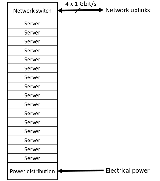
Figure 13.2: A rack containing 16 servers

Each server connects to the rack network switch with a 1 Gbit/s Ethernet cable. The rack in this example connects to the higher-level WSC network environment with four 1 Gbit/s Ethernet cables. Servers within the rack communicate with each other through the rack switch at the full 1 Gbit/s Ethernet data rate. Since there are only four 1 Gbit/s external connections leading from the rack, all 16 servers obviously cannot communicate at full speed with systems external to the rack. In this example, the rack connectivity is oversubscribed by a factor of 4. This means the external network capacity is one quarter of the peak communication speed of the servers within the rack.

Racks are organized into clusters that share a second-level cluster switch. The following diagram represents a configuration in which four racks connect to each cluster-level switch that, in turn, connects to the WSC-wide network:

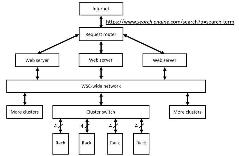
Figure 13.3: WSC internal network

In the WSC configuration of Figure 13.3, a user request arrives over the internet and is initially processed by a routing device that directs the request to an available web server. The server receiving the request is responsible for overseeing the search process and sending the response back to the user.

Multiple web servers are online at all times to provide load sharing and redundancy in case of failure. Figure 13.3 shows three web servers, but a busy WSC may have many more servers in operation simultaneously. The web server parses the search request and forwards queries to the appropriate index servers in the rack clusters of the WSC. Based on the terms being searched, the web server directs index lookup requests to one or more index servers for processing.

To perform efficiently and reliably, the WSC must maintain multiple copies of each subset of the index database, spread across multiple clusters, to provide load sharing and redundancy in case of failures at the server, rack, or cluster level.

Index lookups are processed by the index servers and relevant target page text is collected from document servers. The complete set of search results is assembled and passed back to the responsible web server. The web server then prepares the complete response and transmits it to the user.

The configuration of a real-world WSC will contain additional complexity beyond what is shown in Figure 13.2 and Figure 13.3. Even so, these simplified representations permit us to appreciate some of the important capabilities of a WSC implementing an internet search engine workload.

In addition to responding to user search requests, the search engine must regularly update its database to remain relevant to the current state of web pages across the internet. Search engines update their knowledge of web pages using applications called web crawlers. A web crawler begins with a web page address as its starting point, reads the targeted page, and parses its content. The crawler stores the page text in the search engine document database and extracts any links it contains. For each link it finds, the crawler repeats the page reading, parsing, and link-following process. In this manner, the search engine builds and updates its indexed database of internet content.

This subsection summarized a conceptual WSC design configuration, which is based on racks filled with commodity computing components. The next section examines the measures the WSC must take to detect component failures and compensate without compromising the overall quality of service.

Hardware fault management

As we’ve seen, WSCs contain thousands of computer systems. We can expect hardware failures will occur on a regular basis, even if more costly components have been selected to provide a higher, but not perfect, level of reliability.

As an inherent part of the multilevel dispatch, processing, and return of results implied in Figure 13.3, each server sending a request to a system at a lower level of the diagram must monitor the responsiveness and correctness of the system assigned to process the request. If the response is unacceptably delayed, or if it fails to pass validity checks, the lower-level system must be reported as unresponsive or misbehaving.

When such an error is detected, the requesting system immediately re-sends the request to a redundant server for processing. Some response failures may be due to transient events such as a momentary processing overload. If the lower-level server recovers and continues operating properly, no response is required.

If a server remains persistently unresponsive or erroneous, a maintenance request must be issued to troubleshoot and repair the offending system. When a system is identified as unavailable, WSC management (both the automated and human portions) may choose to bring up a system to replicate the failed server from a pool of backup systems and direct the replacement system to begin servicing requests from users.

Electrical power consumption

One of the major cost drivers of a WSC is electrical power consumption. The primary consumers of electricity in a WSC are the servers and networking devices that perform data processing for end users, as well as the air conditioning system that keeps those systems cool.

To keep the WSC electricity bill to a minimum, it is critical to only turn on computers and other power-hungry devices when there is something useful for them to do. The traffic load to a search engine varies widely over time and may spike in response to events in the news and on social media. A WSC must maintain enough servers to support the maximum traffic level it is designed to handle. When the total workload is below the maximum, any servers that do not have work to do must be powered down.

A lightly loaded server consumes a significant amount of electrical power. For best efficiency, the WSC management system should completely turn off servers and other devices when they are not needed. As the traffic load increases, servers and associated network devices can be powered up and brought online quickly to maintain the required quality of service.

The WSC as a multilevel information cache

We examined the multilevel cache architecture employed in modern processors in Chapter 8, Performance-Enhancing Techniques. To achieve optimum performance, a web service such as a search engine must employ a caching strategy that, in effect, adds levels to those that already exist within the processor.

To achieve the best response time, an index server should maintain a substantial subset of its index data in an in-memory database. By selecting content for in-memory storage based on historic usage patterns, as well as recent search trends, a high percentage of incoming searches can be satisfied without the need to access disk storage.

To make the best use of an in-memory database, the presence of a large quantity of DRAM in each server is clearly beneficial. The selection of the optimum amount of DRAM to install in each index server is dependent upon attributes such as the relative cost of additional DRAM per server in comparison to the cost of additional servers containing less memory, as well as the performance characteristics of more servers with less memory relative to fewer servers with more memory.

We won’t delve any further into such analysis, other than to note that such evaluations are a core element of WSC design optimization.

If we consider DRAM to be the first level of WSC-level caching, the next level is the local disk located in each server. For misses of the in-memory database, the next place to search is the server’s disk. If the result is not found in the local disk, the next search level takes place in other servers located in the same rack. Communications between servers in the same rack can run at full network speed (1 Gbit/s in our example configuration).

The next level of search extends to racks within the same cluster. Bandwidth between racks is limited by the oversubscription of the links between racks and the cluster switch, which limits the performance of these connections. The final level of search within the WSC stretches across clusters, which likely has further constraints on bandwidth.

A large part of the challenge of building an effective search engine infrastructure is the development of a high-performance software architecture. This architecture must satisfy a high percentage of search requests by the fastest, most localized lookups achievable by the search engine index servers and document servers. This means a high percentage of search lookups must be completed via in-memory searches in the index servers.

Deploying a cloud application

In this section, we walk through the steps to develop and deploy a simple web application on the Microsoft Azure cloud platform. This demonstrates how developers take full advantage of large and complex WSC service providers using readily available development tools. This example uses software tools and a cloud service that are available at no cost:

1. Visit https://azure.microsoft.com/en-us/free/ and create a free Azure account. Azure is a cloud computing service provided by Microsoft.
2. Visit https://nodejs.org/en/ and install Node.js. Node.js is a runtime environment for web server applications written in the JavaScript language.
3. Visit https://code.visualstudio.com/ and install Visual Studio Code. Visual Studio Code (abbreviated VS Code) is a multi-language source code editor.
4. Visit https://marketplace.visualstudio.com/items?itemName=ms-azuretools.vscode-azureappservice and install the Azure App Service for VS Code. Azure App Service is an extension to VS Code that assists with creating and deploying web applications in Azure.

The following instructions are demonstrated on a Windows host operating system, but similar (or identical in many cases) commands will work on Linux hosts.

After installing the tools, open a Windows Command Prompt and enter the following commands to create a simple web application and run it on your computer:

C:Projects>npx express-generator webapp --view pug
C:Projects>cd webapp
C:Projectswebapp>npm install
C:Projectswebapp>npm start

Open a web browser and navigate to http://localhost:3000. You will see a web page that looks like Figure 13.4:

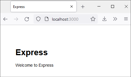
Figure 13.4: Simple Node.js application display

While this application does not do anything objectively useful, the code produced by the preceding steps provides a solid basis for building a sophisticated, scalable web application.

In the following steps, you will deploy this application to the Azure cloud environment using a free Azure account.

1. Start VS Code in the webapp directory:

   C:Projectswebapp>code
   
2. Select the Azure logo as shown in the bottom left corner of Figure 13.5:

   

   Figure 13.5: Adding an application setting

3. Click Sign in to Azure… and complete the process to create a new free account and sign in.
4. Click the cloud icon to the right of APP SERVICE as shown in Figure 13.6. If the icon is not visible, move the cursor to this area and it will appear. When prompted, select the webapp folder:

   

   Figure 13.6: Deploying to the cloud

5. Click + Create new Web App… Advanced. You will be prompted to create a unique name for your application. For example, the name webapp was already in use, but webapp228 was available. You will need to select a different name.
6. Click + Create a new resource group and give it a name. For example, webapp228-rg.
7. You will be prompted to select a runtime stack. In this case, select Node 16 LTS.
8. Select the Windows operating system.
9. Select the geographic location for deployment. For example, West US 2.
10. Select + Create new App Service plan. Give it a name such as webapp228-plan. Select the Free (F1) pricing tier.
11. When prompted with + Create new Application Insights, select Skip for now.
12. Application provisioning in Azure will begin and will take some time. When prompted Always deploy the workspace “webapp” to “webapp228”? select Yes.
13. In VS Code, expand the APP SERVICE node then expand webapp228. Right-click Application Settings. Select Add New Setting… as shown in Figure 13.7.

    

    Figure 13.7: Adding an application setting

14. Enter SCM_DO_BUILD_DURING_DEPLOYMENT as the setting key and true as the setting value. This step will generate a web.config file automatically. This file is required for deployment.
15. Select the cloud icon next to APP SERVICE again and deploy the application.
16. After deployment completes, click Browse Website to open the website in your browser. In this example, the URL for the website is https://webapp228.azurewebsites.net/. This is a publicly accessible website, available to anyone on the internet.

These steps demonstrated the procedure for building and deploying a simple web application to a full-featured cloud environment. By deploying to the Azure environment, our application takes full advantage of Azure cloud platform capabilities that provide performance, scalability, and security.

The next section looks at the high-performance architectures employed in dedicated neural network processors.

Neural networks and machine learning architectures

We briefly studied the architecture of neural networks in Chapter 6, Specialized Computing Domains. This section examines the inner workings of a high-performance, dedicated neural net processor.

Intel Nervana neural network processor

In 2019, Intel announced the release of a pair of new processors, one optimized for the task of training sophisticated neural networks and the other for using trained networks to conduct inference, which is the process of generating neural network outputs given a set of input data.

The Nervana neural network processor for training (NNP-T) is essentially a miniature supercomputer tailored to the computational tasks required in the neural network training process. The NNP-T1000 is available in the following two configurations:

• The NNP-T1300 is a dual-slot PCIe card suitable for installation in a standard PC. It communicates with the host via PCIe 4.0 x16. It is possible to connect multiple NNP-T1300 cards within the same computer system or across computers using cables.
• The NNP-T1400 is a mezzanine card suitable for use as a processing module in an Open Compute Project (OCP) accelerator module (OAM). A mezzanine card is a circuit card that plugs into another plug-in circuit card such as a PCIe card. OAM is a design specification for hardware architectures that implement artificial intelligence systems requiring high module-to-module communication bandwidth. Development of the OAM standard has been led by Facebook, Microsoft, and Baidu. Up to 1,024 NNP-T1000 modules can be combined to form a massive NNP architecture with extremely high-speed serial connections among the modules.

The NNP-T1300 fits in a standard PC and is something an individual developer might use. A configuration of multiple NNP-T1400 processors, on the other hand, quickly becomes very costly and begins to resemble a supercomputer in terms of performance.

The primary application domains for powerful NNP architectures such as Nervana include natural language processing (NLP) and machine vision. NLP performs tasks such as processing sequences of words and attempting to extract the meaning behind them and generating natural language for computer interaction with humans. When you call a company’s customer support line and a computer asks you to talk to it, you are interacting with an NLP system.

Machine vision is a key enabling technology for autonomous vehicles. Automotive machine vision systems process video camera feeds to identify and classify road features, road signs, and obstacles, such as vehicles and pedestrians. This processing must produce results in real time to be useful while driving a vehicle.

Building a neural network to perform a human-scale task, such as reading a body of text and interpreting its meaning or driving a car in heavy traffic, requires an extensive training process. Neural network training involves sequential steps of presenting the network with a set of inputs together with the response the network is expected to produce given that input. This information, consisting of pairs of input datasets and known correct outputs, is called the training set. Each time the network sees a new input set and is given the output it is expected to produce from that input, it adjusts its internal connections and weight values slightly to improve its ability to generate correct outputs. For complex neural networks, such as those targeted by the Nervana NNP, the training set might consist of millions of input/output dataset pairs.

The processing required by NNP training algorithms boils down to mostly matrix and vector manipulations. The multiplication of large matrices is one of the most common and most compute-intensive tasks in neural network training. These matrices may contain hundreds or even thousands of rows and columns. The fundamental operation in matrix multiplication is the multiply–accumulate, or MAC, operation we learned about in Chapter 6, Specialized Computing Domains.

Complex neural networks contain an enormous number of weight parameters. During training, the processor must repetitively access these values to compute the signal strengths associated with each neuron in the model and make training adjustments to the weights. To achieve maximum performance for a given amount of memory and internal communication bandwidth, it is desirable to employ the smallest usable data type to store each numeric value. In most applications of numeric processing, the 32-bit IEEE single-precision, floating-point format is the smallest data type used. When possible, it can help to use an even smaller floating-point format.

The Nervana architecture employs a specialized floating-point format for storing network signals. The bfloat16 format is based on the IEEE-754 32-bit single-precision, floating-point format, except the mantissa is truncated from 24 bits to 8 bits. The Floating-point mathematics section in Chapter 9, Specialized Processor Extensions, discussed the IEEE-754 32-bit and 64-bit floating-point data formats in some detail.

The reasons for using the bfloat16 format instead of the IEEE-754 half-precision 16-bit floating-point format for neural network processing are as follows:

• The IEEE-754 16-bit format has a sign bit, 5 exponent bits, and 11 mantissa bits, one of which is implied. Compared to the IEEE-754 single-precision (32-bit), floating-point format, this half-precision format loses three bits in the exponent, reducing the range of numeric values it can represent to one-eighth the range of 32-bit floating point.
• The bfloat16 format retains all eight exponent bits of the IEEE-754 single-precision format, allowing it to cover the full numeric range of the IEEE-754 32-bit format, though with substantially reduced precision.

Based on research findings and customer feedback, Intel suggests the bfloat16 format is most appropriate for deep learning applications because the greater exponent range is more critical than the benefit of a more precise mantissa. In fact, Intel suggests the quantization effect resulting from the reduced mantissa size does not significantly affect the inference accuracy of bfloat16-based network implementations in comparison to IEEE-754 single-precision implementations.

The fundamental data type used in ANN processing is the tensor, which is represented as a multidimensional array. A vector is a one-dimensional tensor, and a matrix is a two-dimensional tensor. Higher-dimension tensors can be defined as well. In the Nervana architecture, a tensor is a multidimensional array of bfloat16 values. The tensor is the fundamental data type of the Nervana architecture – the NNP-T operates on tensors at the instruction set level.

The most compute-intensive operation performed by deep learning algorithms is the multiplication of tensors. Accelerating these multiplications is the primary goal of dedicated ANN processing hardware such as the Nervana architecture. Accelerating tensor operations requires not just high-performance mathematical processing; it is also critical to transfer operand data to the core for processing in an efficient manner and move output results to their destinations just as efficiently. This requires a careful balance of numeric processing capability, memory read/write speed, and communication speed.

Processing in the NNP-T architecture takes place in tensor processor clusters (TPCs), each of which contains two multiply–accumulate (MAC) processing units and 2.5 MB of high-bandwidth memory. High-bandwidth memory (HBM) differs from DDR SDRAM by stacking several DRAM die within a package and providing a much wider (1,024 bits in comparison to 64 bits for DDR) data transfer size. Each MAC processing unit contains a 32 x 32 array of MAC processors operating in parallel.

An NNP-T processor contains up to 24 TPCs, running in parallel, with high-speed serial interfaces interconnecting them in a fabric configuration. The Nervana devices provide high-speed serial connections to additional Nervana boards in the same system and to Nervana devices in other computers.

A single NNP-T processor can perform 119 trillion operations per second (TOPS). The following table shows a comparison between the two processors:

Table 13.3: Features of the NNP T-1000 processor configurations

The Nervana neural network processor for inference (NNP-I) performs the inference phase of neural network processing. Inference consists of providing inputs to pretrained neural networks, processing those inputs, and collecting the outputs from the network. Depending on the application, the inference process may involve repetitive evaluations of a single, very large network on time-varying input data, or it may involve applying many different neural network models to the same set of input data at each input update.

The NNP-I is available in two form factors:

• A PCIe card containing two NNP I-1000 devices. This card is capable of 170 TOPS and dissipates up to 75 W.
• An M.2 card containing a single NNP I-1000 device. This card is capable of 50 TOPS and dissipates just 12 W.

The Nervana architecture is an advanced, supercomputer-like processing environment optimized for training neural networks and performing inferencing on real-world data using pretrained networks.

Summary

This chapter presented several computer system architectures tailored to particular user needs and identified some key features associated with each of them. We looked at application categories including smartphones, gaming-focused personal computers, warehouse-scale computing, and neural networks. These examples provided a connection between the more theoretical discussions of computer and systems architectures and components presented in earlier chapters and the real-world implementations of modern, high-performance computing systems.

Having completed this chapter, you should understand the decision processes used in defining computer architectures to support specific user needs. You have gained insight into the key requirements driving smart mobile device architectures, high-performance personal computing architectures, warehouse-scale cloud-computing architectures, and advanced machine learning architectures.

The next chapter presents the categories of cybersecurity threats modern computer systems face and introduces computing architectures suitable for applications that require an exceptional assurance of security, such as national security systems and financial transaction processing.

Exercises

1. Draw a block diagram of the computing architecture for a system to measure and report weather data 24 hours a day at 5-minute intervals using SMS text messages. The system is battery powered and relies on solar cells to recharge the battery during daylight hours. Assume the weather instrumentation consumes minimal average power, only requiring full power momentarily during each measurement cycle.
2. For the system of Exercise 1, identify a suitable commercially available processor and list the reasons that processor is a good choice for this application. Factors to consider include cost, processing speed, tolerance of harsh environments, power consumption, and integrated features such as RAM and communication interfaces.

Join our community Discord space

Join the book’s Discord workspace for a monthly Ask me Anything session with the author: https://discord.gg/7h8aNRhRuY