16

Self-Driving Vehicle Architectures

This chapter describes the capabilities of self-navigating vehicle-processing architectures. It begins with a discussion of the types of sensors and data a self-driving vehicle receives as input while driving. We continue with a discussion of the requirements for ensuring the safety of the autonomous vehicle and its occupants, as well as for other vehicles, pedestrians, and stationary objects. Next is a description of the types of processing required for effective vehicle control. The chapter concludes with an overview of an example self-driving computer architecture.

After completing this chapter, you will have learned the basics of the computing architectures used by self-driving vehicles and will understand the types of sensors used by these vehicles. You will be able to describe the types of processing required by self-driving vehicles and will understand the safety issues associated with self-driving vehicles.

The following topics will be presented in this chapter:

• Overview of self-driving vehicles
• Safety concerns of self-driving vehicles
• Hardware and software requirements for self-driving vehicles
• Autonomous vehicle computing architecture

Technical requirements

The files for this chapter, including answers to the exercises, are available at https://github.com/PacktPublishing/Modern-Computer-Architecture-and-Organization-Second-Edition.

Overview of self-driving vehicles

Several major motor vehicle manufacturers and technology companies are actively pursuing the development and sale of fully self-driving, or autonomous, motor vehicles. The utopian vision of safe, entirely self-driving vehicles beckons us to a future in which commuters are free to relax, read, or even sleep while in transit and the likelihood of being involved in a serious traffic accident is drastically reduced from the hazardous situation of today.

While this is the dream, the current state of self-driving vehicles remains far from this goal. Experts in the field predict it will take decades to fully develop and deploy the technology to support the widespread use of fully autonomous transportation.

To understand the requirements of autonomous driving systems, we begin with the inputs a human driver provides to control the operation of a current-generation motor vehicle. These are:

• Gear selection: For simplicity, we assume the presence of an automatic transmission that allows the driver to select between park, forward, and reverse
• Steering: The input for this is the steering wheel
• Accelerator: Pressing a floor pedal accelerates the vehicle in the direction selected by the gearshift
• Brake: Whether the vehicle is moving forward or backward, pressing the brake pedal slows the vehicle and eventually brings it to a stop

To achieve the goals of fully autonomous driving, technology must advance to the point that control of all four of these inputs can be entrusted to the sensors and computing systems present in the automated vehicle.

To understand the current state of self-driving vehicle technology in relation to the goal of fully autonomous driving, it is helpful to refer to a scale that defines the transitional steps from entirely driver-controlled vehicles to a fully autonomous architecture. This is the subject of the next section.

Driving autonomy levels

The Society of Automotive Engineers (SAE) has defined six levels of driving automation (see https://www.sae.org/standards/content/j3016_202104/), covering the range from no automation whatsoever to fully automated vehicles that have no human driver. These levels are:

• Level 0 – No driving automation: This is the starting point, describing the way motor vehicles have operated since they were first invented. At Level 0, the driver is responsible for all aspects of vehicle operation, which includes reaching the intended destination while ensuring the safety of the vehicle, its occupants, and everything outside the vehicle.

  Level 0 vehicles may contain safety features such as a forward collision warning and automated emergency braking. These features are considered Level 0 because they do not control the vehicle for sustained periods of time.

• Level 1 – Driver assistance: A Level 1 driving automation system can perform either steering control or acceleration/deceleration control for a sustained period, but not both functions simultaneously. When using Level 1 driver assistance, the driver must continuously perform all driving functions other than the single automated function. Level 1 steering control is called Lane-Keeping Assistance (LKA). Level 1 acceleration/deceleration control is called Adaptive Cruise Control (ACC). When using a Level 1 driver assistance feature, the driver is required to remain continuously alert and ready to take full control.
• Level 2 – Partial driving automation: Level 2 driving automation systems build upon the capabilities of Level 1 by performing simultaneous steering control and acceleration/deceleration control. As in Level 1, the driver is required to always remain alert and ready to take full control.
• Level 3 – Conditional driving automation: A Level 3 driving automation system can perform all driving tasks for sustained periods of time. A driver must always be present and must be ready to take control if the automated driving system requests human intervention. The primary difference between Level 2 and Level 3 is that in Level 3, the driver is not required to continuously monitor the performance of the automated driving system or maintain awareness of the situation outside the vehicle. Instead, the human driver must always be ready to respond to requests for intervention from the automated driving system.
• Level 4 – High driving automation: A Level 4 automated driving system can perform all driving tasks for sustained periods of time and is also capable of automatically reacting to unexpected conditions in a way that minimizes the risk to the vehicle, its occupants, and others outside the vehicle. This risk minimization process is referred to as driving task fallback, and it may involve actions that result in avoiding risk and resuming normal driving or performing other maneuvers such as bringing the vehicle to a stop at a safe location. A human driver may take over control of the vehicle in response to driving task fallback, or at other times if desired. However, unlike the lower driving automation levels, there is no requirement for anyone in the Level 4 vehicle to remain ready to take over control of the vehicle while it is in operation. It is also not required that vehicles with Level 4 automation include operating controls for human drivers. The primary use case for Level 4 driving automation is in applications such as taxis and public transportation systems where vehicle operation is constrained to a specific geographic region and a known set of roads.
• Level 5 – Full driving automation: In a Level 5 vehicle, all driving tasks are always performed by the automated driving system. There is no need for control inputs that would allow a human driver to operate the vehicle—all vehicle occupants are passengers. A Level 5 driving system must be capable of operating a vehicle on all road types, at all times of day, and in all weather conditions in which a responsible and typically skilled human driver would be able to drive safely. The only driving-related task the human occupants of the vehicle perform is selecting a destination.

In 2021, most vehicles on the road are at Level 0. Many newer vehicle models contain Level 1 and Level 2 automation features. There have been almost no Level 3 systems approved for operation in countries around the world. The Level 3 systems that have received regulatory approval are typically limited to specific operating conditions such as driving in heavy traffic on highways.

An important distinction in the performance requirements for autonomous vehicles compared to many traditional computing applications such as smartphones and web servers is the very real potential for autonomous vehicles to injure and kill vehicle occupants and others outside the vehicle. This is the topic of the next section.

Safety concerns of self-driving vehicles

At all times when some level of autonomous control is active in a moving motor vehicle, the algorithms behind the autonomous behavior must continuously apply a hierarchical set of requirements to meet the needs of passengers while making every effort to avoid negative outcomes, such as collisions with other objects.

The highest priority encoded in autonomous vehicle algorithms must always be to ensure the safety of the vehicle, its occupants, and others in the vicinity. Consider the alternative: if the vehicle’s highest priority was to get its passengers to the requested destination, the vehicle would interpret this as a license to run through red lights and strike pedestrians if those actions result in the quickest path to the destination.

The vehicle not only needs to predict and manage its path through the numerous obstacles that present themselves; it must also ensure that all of its safety-critical components are operating properly and are receiving valid input data. This means that if vital sensors such as video cameras suffer degradation from a buildup of snow or dirt that prevents effective sensor operation, the vehicle algorithms must bring the system to a state of minimum risk. In this situation, the vehicle may take steps to ensure safety by notifying the driver to take control or by bringing the vehicle to a stop at a safe location.

Because it is critical that autonomous vehicles behave in a safe manner, approval for autonomous vehicles to operate on public roads is required by government regulatory agencies responsible for road safety. It is not generally possible for an individual developer or company to build an autonomous vehicle and allow it to operate on roads without this kind of approval. If someone does this and the vehicle ends up causing an accident or injury, the legal liability for the event may be assigned to the vehicle’s occupants or to the party responsible for allowing the vehicle to operate on the road.

Various academic and commercial efforts have completed some of the steps of technological development required for autonomous driving, but a fully capable, fully autonomous vehicle design has yet to be fielded. The following four stages provide a rough guide to the types of autonomous driving capabilities that have been demonstrated and that will be required to reach Level 5 autonomy:

• Stage 1 – Road following: A road-following automated driving system can detect and follow road markings such as lane lines and can even detect texture changes between the road surface and the shoulder on unmarked roads. A driving system that merely maintains the position within a lane does not perform driving necessities like obeying traffic lights and avoiding other vehicles.
• Stage 2 – Obeying traffic rules: A driving automation system at this stage can perform lane keeping while also detecting and responding correctly to driving directions provided by road signs and signal lights. A system with this level of capability can reliably react to signs providing driving information such as a speed limit or a requirement to yield at an intersection.
• Stage 3 – Obstacle avoidance: A driving system capable of obstacle avoidance performs lane keeping and obeys traffic signals while also detecting all significant objects in the vehicle’s vicinity, stationary or moving, and responds appropriately to minimize risk to all. Obstacles include other motor vehicles, cyclists, pedestrians, animals, road construction, debris on the roadway, and other unusual driving situations such as flooded or washed-out roads.
• Stage 4 – Handling edge cases reliably: While it may seem that an automated driving system that handles the first three stages of capability listed here would be of sufficiently high quality to put into operation, perhaps the most challenging aspect of automated driving may be ensuring the system can deal properly with rare but consequential situations where a human driver would be expected to respond in an appropriate manner. For example, suppose flooding has caused a portion of a bridge to collapse into a river.

  A car driven by a human crossing the bridge would ideally come to a stop when the driver observes that a section of the bridge is missing. To be confident of the capabilities of an automated driving system, passengers in an autonomous vehicle must trust it will respond appropriately in all situations where a competent human driver would be able to effectively minimize risk to everyone inside and outside the vehicle.

• A more mundane example of these capabilities occurs when two vehicles pull up to a four-way stop from different directions at nearly the same time. One driver may motion to the other with a hand signal to proceed through the intersection. When the second driver is an autonomous system, will that system detect the gesture and respond appropriately?

While achieving the Stage 4 ability to respond to rare but dangerous events may seem to be a logical extension of the capabilities described in the first three stages, this scenario in fact presents a formidable challenge for an automated driving system. As we’ll see later in this chapter, neural networks are the primary technology currently in use for implementing automated driving systems. Neural networks learn from a series of example situations presented to them along with the “correct” answer the network should produce in each situation. These networks have shown a tremendous ability to generalize from the situations presented to them and respond correctly to novel situations that lie within the scope of the learning situations the network has observed.

The process of dealing with situations that are in some sense “in between” the network learning scenarios is called interpolation. Problems arise when the neural networks attempt to generalize to scenarios that lie outside the scope of their learning scenarios. This is called extrapolation. A neural network’s extrapolated response to a novel situation may or may not be something a competent human driver would consider to be correct. Dealing effectively with the very large number of rare but possible driving scenarios that human drivers experience daily may be the greatest challenge facing the development of autonomous driving systems.

The next section introduces the data inputs provided to autonomous driving systems by the various sensors installed in the vehicle.

Hardware and software requirements for self-driving vehicles

Human drivers must sense the state of their vehicles and constantly evaluate the surrounding environment, keeping track of stationary and moving obstacles. The primary means of gathering this information is through vision.

Using eyesight, a competent driver monitors vehicle instrumentation, principally the speedometer, and scans the surrounding environment to perform lane keeping, maintain appropriate spacing from other vehicles, obey traffic signs and signals, and avoid any obstacles on or near the road surface.

Human drivers rely on other senses to a lesser degree, including the use of hearing to detect signals such as car horns and railway crossings. The sense of touch comes into play as well, for example when bump strips are installed on a highway surface to warn of an upcoming intersection. The sense of touch can also assist when an inattentive driver drifts off the roadway and onto the shoulder, which typically has a significantly different texture from the road surface.

Sight, hearing, and touch are the only inputs a human driver uses while driving. Looked at in one way, this demonstrates that the information input provided by these senses enables human drivers to travel billions of miles each day, largely successfully. Viewed differently, significant gaps obviously remain in the processes of sensing and executing appropriate responses to hazardous situations as evidenced by the thousands of deaths that occur daily in traffic accidents.

To be accepted by the driving public, autonomous driving systems must not be merely as safe as human drivers—they must be demonstrably far superior to humans in terms of the rate of traffic accidents per mile traveled. This high level of performance will be necessary because many human drivers will be reluctant to turn over control to an automated system until they have been convinced the system is superior to their own (perhaps imagined) high level of driving skill.

The next section introduces the types of sensors used in autonomous driving systems and their contributions to meeting the goals of safety and reliability.

Sensing vehicle state and the surroundings

Autonomous driving sensors must accurately measure the state of the vehicle itself as well as the location and velocity (velocity is the combination of speed and direction of motion) of all significant objects in the vehicle’s vicinity. The following sections describe the primary sensor types used in current generations of autonomous vehicle designs.

GPS, speedometer, and inertial sensors

An autonomous vehicle must continuously maintain awareness of its state, which includes its location, direction of movement, and speed. Vehicle location information is used for low-level driving tasks like lane keeping, and for higher-level functions such as developing a route to a destination.

Low-level location measurements enable information to be derived from lidar data or from video camera images that provide information including the vehicle’s position relative to lane-marking lines. This information is high-resolution (meaning accuracy is measured in centimeters) and is updated at a high rate (perhaps dozens or even hundreds of times per second), enabling smooth and continuous responses by the driving system to changing conditions.

The information provided by a Global Positioning System (GPS) sensor is updated less frequently (perhaps a few times per second) and may have much lower accuracy, with position errors of multiple meters. The information provided by a GPS receiver is ideal for use in route planning, but it is likely to provide too coarse of a measurement and to be updated too infrequently to be of use for keeping a vehicle centered in a lane.

GPS receivers have a notable performance limitation because they rely on the continuous reception of satellite signals to enable their operation. In situations where visibility of the sky from the vehicle is impaired, perhaps on a road with dense tree cover, in the urban canyon of a city center, or in a tunnel, the GPS receiver may not work at all.

The vehicle’s speedometer normally provides an accurate measurement of vehicle speed based on tire rotation rate. At times the speedometer measurement may be an inaccurate representation of the vehicle speed due to tire slippage, perhaps resulting from the presence of mud or ice on the roadway. As a backup to the speedometer, GPS provides an accurate measurement of vehicle speed whenever it is receiving the necessary satellite signals. In this situation, divergence between the vehicle speedometer reading and the speed measured by the GPS may be an indication of tire slippage, which is an unsafe condition.

Modern vehicles often contain inertial sensors in the form of accelerometers and, in some cases, a gyroscope. An accelerometer measures the acceleration, or rate of change of velocity, along a single axis of motion. Humans sense acceleration as the force pressing them back into the seat while a vehicle is speeding up and as the force pushing them sideways during an aggressive turn.

Motor vehicles typically contain two accelerometers: one to measure acceleration and deceleration along the forward-reverse axis of motion, and a second measuring acceleration along the side-to-side axis of motion. The accelerometer measuring side-to-side acceleration measures the inertial effects of turns. A gyroscope can be used to measure the vehicle’s rate of turn directly.

Accelerometers can provide measurements at very high rates and are used for purposes such as deploying air bags within milliseconds after a collision has been detected. The accelerometers and gyroscope in a vehicle track its orientation and velocity, enabling it to maintain an accurate understanding of its relationship to its surroundings.

Using an algorithm called a Kalman filter, it is possible to combine measurements from multiple sources like the GPS receiver and inertial sensors with a mathematical model of the physical laws that constrain the motion of objects such as an automobile. The Kalman filtering process recognizes that each measurement contains some error and that the mathematical model is an imperfect representation of the dynamic behavior of the vehicle. By incorporating the statistical error characteristics of the sensors and the range of unpredictable behaviors a vehicle can experience (resulting from acceleration, braking, and steering inputs as well as from external effects such as driving up and down hills), the Kalman filter synthesizes the available information to produce an estimate of the vehicle’s state that is significantly more accurate than the information received from any sensor or the mathematical model by itself.

The GPS, speedometer, and inertial sensors provide an estimate of the vehicle’s state. To drive safely and reach a requested destination, an autonomous driving system must also sense the environment surrounding it. The sensors that perform this function are the subjects of the following sections.

Video cameras

Some autonomous driving systems employ an array of video cameras as the primary sensor of the external environment. The video cameras used in these vehicles have features that are familiar to users of consumer-grade digital video cameras, including handheld devices and the video cameras in smartphones. An autonomous vehicle video camera is a moderately high-resolution device, typically 1,920x1,080 pixels. A vehicle may have several cameras located around its periphery with overlapping fields of view.

The use of multiple cameras highlights one improvement of autonomous vehicles over human-driven vehicles: vision systems used in autonomous vehicles are capable of simultaneously and continuously monitoring activity around the vehicle in all directions. Human drivers, in comparison, can only look in one direction at a time, with some limited peripheral vision across a greater field of view. The presence of internal and external mirrors in human-driven vehicles helps to mitigate this inherent limitation of human vision, though there are typically substantial blind spots that human drivers must be cognizant of and incorporate into their situational awareness.

The greatest challenge associated with using video cameras in autonomous driving systems is that the video images output by these devices are not directly useful in performing driving tasks. Substantial processing must be performed to identify significant features in the images, combine those features to recognize individual objects, and then understand what the objects are doing and react appropriately. We will discuss the processing of video images in autonomous driving systems in the Perceiving the environment section later in this chapter.

Radar

One limitation of video cameras in autonomous driving systems is that they provide a flat, two-dimensional image of the scene viewed by the camera. Without substantial further processing, it is not possible to tell if the portion of the scene represented by any individual pixel is close to the vehicle (and therefore potentially an obstacle that requires an immediate reaction) or something that is far away and is of no relevance to the driving task.

The technology of radio detection and ranging (radar) provides a solution to part of this problem. A radar system repetitively sends out pulses of electromagnetic energy into the environment and listens for echoes of those signals bouncing off objects in its vicinity.

A radar system can detect objects and provide measurements of the direction to each object as well as the range to those objects. It can also measure the speed of objects relative to the vehicle carrying the radar system. A radar system can track a vehicle several hundred feet ahead and maintain a safe following distance when used as part of an ACC.

Radar systems have some significant limitations, however. Compared to a video camera, the scene perceived by a typical automotive radar system is much blurrier and has lower resolution. Radar systems are also prone to noisy measurements, which reduces confidence in the quality of the information they provide.

Despite those limitations, radar sensors perform without degradation in situations where video cameras often fail, such as in heavy rain, snow, and dense fog.

Lidar

Instead of using video cameras, some autonomous vehicle developers have elected to rely on lidar systems for determining vehicle location and orientation and detecting objects in the vehicle’s vicinity. A light detection and ranging (lidar) sensor uses a laser to scan the area around the vehicle and collect data from the reflections received from surfaces and objects.

Each measurement by a lidar device represents the distance from the lidar laser illuminator to a surface that reflects some of the laser energy back to the lidar sensor. The direction of the laser beam relative to the vehicle at the time of each sample is known to the lidar processing software. The distance to the reflecting point and back is calculated by measuring the time between when the laser pulse is emitted and the time the echo arrives at the lidar sensor, which is referred to as the pulse’s time of flight. The round-trip distance traveled by the pulse is equal to the pulse’s time of flight multiplied by the speed of light through the atmosphere.

By collecting measurements in rapid succession in all directions around the vehicle, a three-dimensional set of points called a point cloud is developed. This point cloud represents the distance from the lidar sensor to surrounding surfaces, including the road surface, buildings, vehicles, trees, and other types of objects.

Sonar

Sound navigation and ranging (sonar) performs a function that is intuitively similar to radar and lidar systems, except sonar systems emit pulses of sound rather than electromagnetic waves.

Sonar systems generally operate at much shorter ranges than radar and lidar systems and are mainly used to detect obstacles in close-quarters situations, like when parking between other vehicles or for detecting when a vehicle in an adjacent lane on a highway is approaching uncomfortably close to the vehicle.

Perceiving the environment

As sensors collect raw information about the vehicle and its surroundings, the sensor output information is not immediately usable for performing effective vehicle control. Several stages of processing must be performed to convert raw sensor measurements into actionable information that can be used for autonomous driving. The following sections describe the processing steps needed to convert sensor data into driving decisions in autonomous vehicles that rely on video cameras and lidar systems as primary sensors. We begin with the processing of images from video cameras using convolutional neural networks.

Convolutional neural networks

Chapter 6, Specialized Computing Domains, briefly introduced the concepts of deep learning and artificial neural networks. To recap, artificial neurons are mathematical models intended to represent the behavior of biological neurons, which are the brain cells responsible for perception and decision making.

In modern autonomous vehicle systems that use video cameras to sense the environment, the leading technology used to extract decision-quality information from video images captured by cameras is the convolutional neural network.

A Convolutional Neural Network (CNN) is a specialized type of artificial neural network that performs a form of filtering called convolution on raw image data to extract information useful for detecting and identifying objects within the image.

An image captured by a video camera is a rectangular grid of pixels. The color of each pixel is represented by a set of red, green, and blue intensities. Each of these intensities is an 8-bit integer ranging from 0 to 255. An intensity of 0 means the corresponding color is not present in the pixel’s color, while 255 represents the maximum intensity for that color. A pixel’s color is represented by the three red, green, and blue values, abbreviated as RGB. Some examples of RGB colors are listed in Table 16.1:

Red Intensity	Green Intensity	Blue Intensity	Color
255	0	0	Red
0	255	0	Green
0	0	255	Blue
0	0	0	Black
255	255	255	White
128	128	128	Gray
255	255	0	Yellow
255	0	255	Magenta
0	255	255	Light Blue

Table 16.1: Examples of RGB colors

A CNN receives as its input the RGB image captured by a video camera as three separate two-dimensional arrays of 8-bit pixel colors, one each for red, blue, and green. We will refer to these as the three color planes of the image.

The CNN then performs convolution filtering on each of the color planes. A convolution filter consists of a rectangular grid of numbers that is typically small, perhaps 2 rows by 2 columns. The convolution operation begins at the top-left corner of each color plane. Mathematically, convolution is performed by multiplying the color intensity at each pixel location by the number at the corresponding location in the convolution filter and then summing the products of these operations over all elements in the filter. The result of this operation is one element of the convolution output. We’ll go through an example shortly to help clarify this process.

The convolution continues by shifting the filter 1 or more pixels to the right, and then repeating the multiplication and summing operations with the image pixels covered at the filter’s new location. This produces the convolution output at the second location in the top row. This process continues all the way across the top row of the image and then the filter shifts back to the left edge and moves downward by 1 or more pixels and repeats the process across the second row in the image. This sequence of shifting the filter, multiplying the filter elements by the pixel color intensities at the filter location, and summing the results continues across the entire image.

Example CNN implementation

We’ll now present a simple example to demonstrate how CNNs work. Let’s say we have an image that is 5x5 pixels and a convolution filter that is 2x2 pixels. We will only look at one of the three color planes, though in real filters, the same operations will be performed separately across all three color planes.

We will shift the filter by 1 pixel to the right and 1 pixel downward each time such movement is required. The distance (in terms of pixels) the convolution filter shifts each time it relocates is called the stride. For simplicity, all pixels and convolution filter elements in the example will be represented as single-digit integers. Table 16.2 contains our example color plane data:

1	4	6	7	8
2	9	2	0	5
8	2	1	4	7
3	9	0	6	8
2	1	4	7	5

Table 16.2: Example color plane data

Table 16.3 contains the convolution filter. Each number in the table is one filter coefficient:

7	2
8	0

Table 16.3: Example convolution filter

We will be using a stride of 1, which means each sequential evaluation of the filter output will shift 1 pixel to the right and then 1 pixel downward and back to the left edge when the right edge of the image has been reached.

For the first filter evaluation, we multiply the pixels in the upper-left corner of the image by the corresponding elements in the convolution filter, as shown in Table 16.4:

1×7	4×2	6	7	8
2×8	9×0	2	0	5
8	2	1	4	7
3	9	0	6	8
2	1	4	7	5

Table 16.4: Multiplication step in convolution

After multiplying the color plane intensities by the convolution filter elements in the 2x2 grid, we add them together, as shown in Equation 16.1:

Equation 16.1: Multiplication and summing steps in convolution

The result of the element-by-element multiplication of the color plane intensities by the filter coefficients, followed by summing each of those results, is one element of our output array, C_1,1, which we place in row 1, column 1 of our output array, as shown in Table 16.5:

31

Table 16.5: First convolution output element

Next, we shift the filter grid one position to the right and perform the multiply-and-sum operation again, as shown in Table 16.6:

1	4×7	6×2	7	8
2	9×8	2×0	0	5
8	2	1	4	7
3	9	0	6	8
2	1	4	7	5

Table 16.6: Multiplication step in convolution

After multiplying the color plane intensities at the second filter location by the convolution filter elements, the result is shown in Equation 16.2:

Equation 16.2: Summing step in convolution

Table 16.7 shows the convolution output after the second element has been inserted at row 1, column 2:

31	112

Table 16.7: Second convolution output element

We continue shifting 1 pixel to the right for each evaluation across the top row. Because our filter is 2 pixels wide and the image is 5 pixels wide, we can only place the filter in 4 locations without running the filter off the image. This is the reason the filter output array has 4 rows and 4 columns.

After the top row of the image is complete, we bring the filter back to the left image edge and move it down 1 pixel to compute the element in row 2, column 1 (C_2,1). This process repeats across the entire image until it ends at the bottom-right corner. For our 5x5 image, the completed output of the convolution operation is shown in Table 16.8:

31	112	72	65
96	83	22	42
84	88	15	90
55	71	44	114

Table 16.8: Result of convolution operation

While this explanation of convolution may have seemed a bit tedious and unenlightening, we are now getting to the good part.

CNNs in autonomous driving applications

These are the most interesting points related to the use of convolution filtering in video image processing for autonomous driving systems:

• Mathematically, convolution consists of the simple operations of multiplication and addition.
• CNNs can be trained in the same way as the Artificial Neural Networks (ANNs) discussed in Chapter 6, Specialized Computing Domains. This training consists of repeated trials that present the neural network with a set of input data along with the “correct” output that should be produced when presented with that data. The training process adjusts the weights within the ANN (and in convolution filters of the CNN) to improve its ability to respond correctly to the given inputs on each iteration.
• As part of the training process, the CNN discovers the best data values to place at each location in its convolution filter tables.

To provide a concrete example, consider the problem of steering a vehicle to remain properly centered within its lane. To train a CNN to perform this task, the general procedure is to record a series of video segments from vehicle cameras together with appropriate steering commands that the autonomous system must attempt to replicate as its output.

The training dataset must provide sufficient variety to ensure the behavior learned by the CNN covers the full range of its intended operating conditions. This means the training data should include straight roads and roads with a variety of curves. The data should also include daytime and nighttime driving, and other conditions that may be encountered, such as different types of weather.

During training, each training example is presented to the network as a video image along with the correct steering response. As the CNN learns how to respond properly to the varying inputs, it adjusts the coefficients in its convolution filters to identify image features that are useful in performing the desired tasks.

One image feature that is particularly useful in autonomous driving is edge detection. Edge detection involves locating the dividing lines that separate distinct portions of the image from one another. For example, the lines painted on roadways are always in a very different color from the road surface to make them highly visible to drivers, both human and autonomous.

The most interesting, even fascinating, attribute of the CNN training process is that by simply presenting video frames of road surfaces to a CNN along with accurate examples of the desired outputs, the CNN will discover image attributes that are useful (such as edges) and build convolution filters automatically that are specifically tuned to identify useful features.

Because the CNN filter is applied repeatedly across the entire image, it is possible for the filter to detect objects wherever they may appear in the image. This is an important feature of autonomous driving because it is not possible to predict the location in a video image where an important object may appear.

Real-world applications of CNNs may contain several convolution filters, each containing different sets of coefficients. Each of these filters is tuned during the training process to seek out different types of relevant features that can be processed in later stages of the network to perform higher-level functions, like identifying stop signs, traffic lights, and pedestrians.

A complete CNN design contains one or more stages of convolution that each operates as described in this section. The initial convolution stage performs filtering to detect simple features like edges, while later stages combine these features to identify more complex objects like a stop sign.

To reliably detect a feature such as a stop sign under varying conditions, the training data must contain images of stop signs as seen from nearby and far away, as well as when looking at it straight on and from off to the side at an angle, all under a variety of lighting and weather conditions.

Within the CNN structure, the data elements computed in each convolution stage pass through an activation function to produce the final output of the stage. Although many types of functions can be used for this purpose, a common activation function is the Rectified Linear Unit function, abbreviated to RELU.

The RELU activation function is a very simple formula: given the table of output values from a convolution operation such as Table 16.8, examine each element. If the element is less than 0, replace it with 0. That’s all there is to it. Our simple example in Table 16.8 does not contain any negative elements, so applying RELU will not change it. In real applications, the RELU activation function provides important benefits, including improved training speed compared to other common activation functions.

Another type of stage used in CNN architectures is the pooling stage. High-resolution images contain a large number of pixels. To keep memory consumption and processing requirements within achievable limits, it is necessary to reduce the quantity of data flowing through the network while retaining the features that lead to the correct recognition of objects within the image. One way to do this is a technique called pooling. Pooling combines multiple elements in an input table into a single element in the output table. For example, each 2x2 pixel subset of Table 16.8 could be combined to reduce the size of the output from that subset to a single numerical value.

There are several ways to combine the pixels within a subset into a single value. One obvious possibility is to compute the average. For the 2x2 pixel region in the upper-left corner of Table 16.8, the average is (31 + 112 + 96 + 83) / 4 = 80.5). While averaging provides a representation that includes effects from all the pixels in the region, this has not proven to be a pooling method providing the best performance in CNNs. Instead, in many cases, simply selecting the maximum value within the region as the pool result has been shown to give good performance. In this example, the maximum value of the selected region is 112.

This technique is referred to as max pooling. Table 16.9 shows the results of applying max pooling with a region size of 2x2 to Table 16.8:

112	72
88	114

Table 16.9: Result of 2x2 max pooling on Table 16.8

To convert a layer from the two-dimensional structure of the video images and the convolutional layers that process the video data into a form suitable for input to a traditional ANN, it is necessary to rearrange the data into a one-dimensional format.

As with the other mathematical operations described earlier, this is a simple procedure. The conversion from a two-dimensional structure to a one-dimensional vector is called flattening. In a flattening layer, the coefficients in the two-dimensional structure are simply transferred sequentially into a vector, which serves as the input to a traditional ANN.

Table 16.10 presents the results of Table 16.9 after the flattening operation has been performed:

112

72

88

114

Table 16.10: Result of flattening on Table 16.9

Table 16.10 is a one-dimensional vector of numeric values that is in a suitable format for use as input to a traditional ANN.

Following the convolutional, pooling, and flattening stages, a CNN implements one or more ANN layers, each of which forms a hidden layer of neurons. These hidden layers are usually fully connected sets of neurons, as shown in Figure 6.5 in Chapter 6, Specialized Computing Domains. Following the hidden layer is an output layer, which presents the final outputs of the network for use in further processing.

When a sufficiently rich set of training data has been combined with an appropriately sized CNN structure capable of learning and retaining the necessary knowledge, it is possible to encode a tremendous amount of information that represents a wide variety of driving situations into the CNN and ANN coefficients.

In a roadworthy autonomous vehicle design, the result of the CNN design and training process is a system that can recognize and identify the object types encountered across the full range of driving situations encountered by drivers daily. This is a tremendously complex task, and it may take several years before the computing technology and software capability (both in the network structure and in the training process) are capable of consistently outperforming human drivers in the tasks of object detection and recognition.

Figure 16.1 presents a basic (Stage 1, as described above) CNN architecture that has shown to be capable of steering an autonomous driving system to remain somewhat centered in a lane on a curving road:

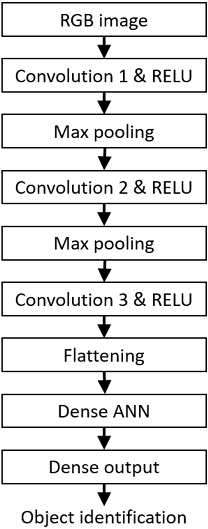
Figure 16.1: CNN layers used in object identification application

The exercises at the end of this chapter develop an example CNN based on the structure of Figure 16.1 that can identify and categorize objects in low-resolution color images with a significant degree of accuracy.

You may wonder how the developer of a CNN for a particular application selects architectural features such as the types and number of layers and other parameters defining the network. In many cases, it is not at all clear what the best combination of layer types and the settings for other network parameters (such as convolution filter dimensions) is for achieving the overall goals of the CNN application.

The types and dimensions of layers and related parameters describing a neural network are referred to as hyperparameters. A hyperparameter is a high-level design feature of a neural network that defines some part of its structure. Hyperparameters are distinct from the weighting factors (see Figure 6.4) on the neural connections, which are defined automatically during the training process.

The selection of hyperparameter values to configure a neural network for a particular application can be considered a search process. The architect of the neural network design can use software tools to test a variety of network architectures composed of different sequences of neural network layer types along with different parameter values associated with each layer, such as the dimensions of convolution filters or the number of neurons in a fully connected layer. This search process comprises a training phase for each network configuration followed by a testing phase to evaluate the performance of the trained network. Network designs that perform the best during the testing phase are retained for further evaluation as the design process moves forward.

In the next section, we’ll look at how lidar is used to perform the functions of determining a vehicle’s location and identifying objects in the surroundings.

Lidar localization

As we discussed earlier, lidar sensors measure the distance to surfaces that reflect some of the transmitted laser energy back to the lidar sensor. The direction of the transmitted laser beam relative to the vehicle at the time of each sample is known to the lidar processing software. The distance to the reflecting point and back is calculated by measuring the time between when the laser pulse is emitted and the time the echo arrives at the lidar sensor, which is referred to as the pulse’s time of flight. The round-trip distance traveled by the pulse is equal to the pulse’s time of flight multiplied by the speed of light.

By collecting measurements in rapid succession in all directions around the vehicle, a point cloud can be formed, which contains the full set of measurements to points in the surroundings.

By comparing the point cloud produced by the lidar sensor to a stored map of surfaces and structures in the vicinity of the vehicle location, the lidar data processing software can adjust and align its measured point cloud to bring it into agreement with the stored map data. This process enables the lidar system to precisely determine its location and orientation relative to the surrounding environment. This process is referred to as localization.

In comparison to video image-based autonomous driving systems, lidar-based driving systems have the following advantages:

• Lidar sensors continuously produce precise three-dimensional maps of the surroundings. This information represents the distance from the sensor to each point in the point cloud. A single video camera produces a two-dimensional image with no information about the distance to any point in the scene.
• Video cameras can be blinded by sunlight or another bright light source. Lidar sensors are much less susceptible to such interference.
• The object detection function in video camera-based systems may fail to identify objects when the perceived color of the object lacks sufficient contrast from the surrounding environment. Lidar systems detect objects in their surroundings regardless of their color.

Lidar systems have the following limitations:

• Lidar systems have substantially less resolution than standard video cameras.
• As with video cameras, the performance of lidar sensors can be impaired by weather conditions such as fog and heavy rain.
• Lidar localization systems only work on roads and in other environments that have been precisely mapped. The database containing the map information must be available to the vehicle while operating. This necessitates an ongoing investment to collect mapping data on the roads used for autonomous driving. The mapping effort must repeat the data collection process to pick up changes such as the construction of new buildings near roadways. When driving on roads that have not been mapped, the lidar system is not available for use by the vehicle.
• Lidar systems tend to be significantly more expensive than video cameras.

There is ongoing competition between automakers and technology companies to develop and deploy autonomous driving systems using different sensing technologies. As of 2021, Tesla has focused its efforts on the use of multiple video cameras to provide the information necessary to perform autonomous driving functions without the need for a precision map of the surrounding environment.

Other companies, including Toyota and Waymo, rely on the use of lidar as the primary system for sensing the environment in concert with a database containing three-dimensional localization data.

Whether an autonomous driving system relies on video cameras or a lidar system, it must identify and track objects over time to perform the functions required for safe driving. This is the subject of the next section.

Object tracking

The output from the perception stage of an autonomous driving system includes a list of objects and their classification (such as a truck or cyclist) derived from video or lidar data. To support the task of driving, additional processing must be performed to maintain a history of objects identified in sequential sensor updates and track the behavior of those objects over time.

Object tracking measures object motion over time and enables the prediction of the future motion of those objects. The results of object motion prediction are used in path planning decisions to maintain safe separation distances from other objects and to minimize the risk of collisions.

Tracking objects over sequential updates permits errors such as spurious object detection within individual scene samples to be identified and corrected if the presence of the possible object cannot be confirmed in later updates.

After developing a dataset describing the state of the vehicle and all the objects relevant to driving the vehicle, the autonomous driving system must make a series of decisions, discussed next.

Decision processing

Using the information provided during the perception stage of sensor data processing, the autonomous driving system decides upon the actions it will execute at each moment to continue safe vehicle operation while making progress toward the requested destination. The basic functions it must support consist of lane keeping, obeying the rules of the road, avoiding collisions with other objects, and planning the vehicle path. These are the topics of the following sections.

Lane keeping

The lane-keeping task requires the vehicle driver (human or autonomous) to continuously monitor the vehicle’s location within the width of the lane it occupies and maintain the vehicle’s position within an acceptable deviation from the center of the lane.

Lane keeping is a straightforward task on a clearly marked road in good weather conditions. On the other hand, an autonomous driving system (or a human driver) may experience significant difficulty staying centered in a lane when lane markings are obscured by fresh snowfall or mud on the road’s surface.

A lidar-based autonomous driving system should experience little or no impairment while navigating a road surface covered by a light layer of snow, as long as lidar measurements of the surroundings continue to provide valid information. A video camera-based system, however, may experience substantial difficulty in this context.

Complying with the rules of the road

Autonomous driving systems must obey all traffic laws and regulatory requirements while operating on public roads. This includes basic functions, like stopping for stop signs and responding appropriately to traffic lights, as well as other necessities, such as yielding the right of way to another vehicle when the situation requires it.

The driving task can become complex when autonomous vehicles must share the road with human-operated vehicles. Humans have developed a range of behaviors for use in driving situations that are intended to make driving easier for everyone. For example, a vehicle on a crowded highway may slow down to provide space for a merging vehicle to enter the roadway.

A successful autonomous driving system must comply with all legal requirements and must also align its behavior with the expectations of human drivers.

Avoiding objects

Autonomous driving systems are required to perceive and respond appropriately to the entire gamut of inanimate objects and living creatures that drivers encounter on roads every day. This includes not only other vehicles, pedestrians, and cyclists—random objects such as ladders, car hoods, tires, and tree limbs also wind up on roads every day. Animals such as squirrels, cats, dogs, deer, cattle, bears, and moose regularly attempt to cross the roads in various regions.

Human drivers generally attempt to avoid striking smaller animals on the road if it can be done without creating an unacceptably dangerous situation. When encountering a large animal, avoiding impact might be necessary to prevent killing the vehicle’s occupants. Autonomous driving systems will be expected to outperform human drivers under all these conditions.

Planning the vehicle path

High-level path planning generates a sequence of connected road segments the vehicle intends to traverse while traveling from its starting point to its destination. GPS-based route planning systems are familiar to drivers of today’s vehicles. Autonomous vehicles use the same approach to develop a planned path to their destination.

Low-level path planning encompasses all the driving actions along the path to the destination. An autonomous driving system must constantly evaluate its surroundings and make decisions such as when to change lanes, when it is safe to enter an intersection, and when to give up trying to turn left onto a very busy street and fall back to an alternate route.

As with all aspects of autonomous driving, the highest goals of path planning are to keep the vehicle occupants and others outside the vehicle safe, obey all traffic laws, and, while accomplishing all that, travel to the destination as quickly as possible.

Autonomous vehicle computing architecture

Figure 16.2 summarizes the hardware components and the processing stages in an autonomous driving system based on the current state of technology, as described in this chapter.

Figure 16.2: Components and processes of an autonomous driving system

We introduced sensor technologies that gather information about the state of the vehicle and its surroundings. This information flows into a Sensing process, which receives data from the sensors, validates that each sensor is performing properly, and prepares the data for perception. The process of Perceiving takes raw sensor data and extracts useful information from it, such as identifying objects in video images and determining their location and velocity. With an accurate understanding of the vehicle’s state and all relevant surrounding objects, the Deciding process performs high-level navigation functions, like selecting which route to take to the destination, as well as low-level functions such as choosing what direction to go at an intersection. The process of Acting on these decisions sends commands to hardware units performing steering, controlling vehicle speed, and providing information to other drivers, most notably by operating the turn signals.

Tesla HW3 Autopilot

To maintain trade secrets, some of the automotive and technology companies working to develop autonomous driving systems have released very limited information about the designs of their systems. Tesla, on the other hand, has been more forthcoming with information about the autonomous driving computer hardware used in their vehicles. Tesla vehicles are currently operating on public roads with so-called full self-driving capabilities using a computer system called Hardware 3.0 (HW3).

The Tesla HW3 processor board contains two fully redundant computing systems, each of which is capable of safely operating the vehicle on its own. The two systems operate in synchrony and continuously compare their outputs. If one of the systems experiences a failure, the second system takes over vehicle operation until a repair can be performed.

The HW3 computer is based on a custom SoC that Tesla developed to optimize system performance for the autonomous driving task. The SoC incorporates substantial resources for neural network computing in addition to traditional capabilities related to image processing and scalar computation.

These are some of the key features of the Tesla HW3 computer:

• The SoC integrated circuit is based on a 14 nm FinFET process with a total of 6 billion transistors. The Fin Field-Effect Transistor (FinFET) technology employs a significant vertical dimension (called the “fin”), which differs from the planar circuit structure of traditional CMOS technology. FinFETs can achieve faster switching times and carry a higher current than traditional CMOS transistors. HW3 was the first automotive application of the 14 nm FinFET technology.
• The HW3 computer uses Low-Power DDR4 (LPDDR4) DRAM. LPDDR4 is a variation of DDR4 DRAM optimized to reduce power consumption for applications such as smartphones and laptop computers. LPDDR4 has lower bandwidth than DDR4 and consumes substantially less power. While a Tesla vehicle has a very large battery compared to a smartphone, the power consumed by the vehicle computer must still be kept to a minimum, and the use of LPDDR4 DRAM helps with that.
• Each SoC contains two neural network accelerators, which together perform 72 TOPS (tera-ops, or trillions of operations per second). These processors execute a CNN for object detection within video camera images.
• Each neural network accelerator has 32 KB of dedicated high-speed SRAM. As we saw in Chapter 8, Performance-Enhancing Techniques, SRAM is much faster than DRAM, but has a significantly higher cost per bit in terms of chip area. This substantial quantity of SRAM provides a performance boost compared to other general-purpose processors that Tesla might have employed instead of the custom SoC.
• For general-purpose computing, each HW3 processor contains three quad-core ARM Cortex A72 64-bit CPUs running at 2.2 GHz.

According to Tesla, the HW3 computer can process an amazing 2,300 frames per second of high-definition video through its CNN architecture. This level of performance is required to support progress toward Tesla’s stated goal of using video camera-based sensing to enable Level 5 autonomous driving.

Autonomous vehicle technology is a rapidly developing field, but the current state of the art in vehicles available for purchase by the public remains significantly short of the goal of driverless operation. It may be several years before vehicles become available that are capable of carrying passengers on public roads without the need for someone to constantly monitor the surroundings through the windshield.

Summary

This chapter presented the capabilities required in self-navigating vehicle-processing architectures. It began by introducing driving autonomy levels and the requirements for ensuring the safety of the autonomous vehicle and its occupants, as well as the safety of other vehicles, pedestrians, and stationary objects. We continued with a discussion of the types of sensors and data a self-driving vehicle receives as input while driving. Next, we discussed the types of processing required for vehicle control. We ended with an overview of the Tesla HW3 computer architecture.

Having completed this chapter, you have learned the basics of the computing architectures used by self-driving vehicles and understand the types of sensors used by self-driving vehicles. You can describe the types of processing required by self-driving vehicles and understand the safety issues associated with self-driving vehicles.

In the next and final chapter, we will develop a view of the road ahead for computer architectures. The chapter will review the significant advances and ongoing trends that have led to the current state of computer architectures and extrapolate those trends to identify some possible future technological directions. Potentially disruptive technologies that could alter the path of future computer architectures will be considered as well. In closing, some approaches will be proposed for the professional development of a computer architect that are likely to result in a future-tolerant skill set.

Exercises

1. If you do not already have Python installed on your computer, visit https://www.python.org/downloads/ and install the current version. Ensure Python is in your search path by typing python –-version at a system command prompt. You should receive a response similar to Python 3.10.3.

   Install TensorFlow (an open source platform for machine learning) with the command (also at the system command prompt) pip install tensorflow. You may need to use the Run as administrator option when opening the command prompt to get a successful installation. Install Matplotlib (a library for visualizing data) with the command pip install matplotlib.

2. Create a program using the TensorFlow library that loads the CIFAR-10 dataset and displays a subset of the images along with the label associated with each image. This dataset is a product of the Canadian Institute for Advanced Research (CIFAR) and contains 60,000 images, each consisting of 32x32 RGB pixels. The images have been randomly separated into a training set containing 50,000 images and a test set of 10,000 images. Each image has been labeled by humans as representing an item in one of 10 categories: airplane, automobile, bird, cat, deer, dog, frog, horse, ship, or truck. For more information on the CIFAR-10 dataset, see the technical report by Alex Krizhevsky at https://www.cs.toronto.edu/~kriz/learning-features-2009-TR.pdf.
3. Create a program using the TensorFlow library that builds a CNN using the structure shown in Figure 16.1. Use a 3x3 convolution filter in each convolutional layer. Use 32 filters in the first convolutional layer and 64 filters in the other two convolutional layers. Use 64 neurons in the hidden layer. Provide 10 output neurons representing an image’s presence in one of the 10 CIFAR-10 categories.
4. Create a program using the TensorFlow library that trains the CNN developed in Exercise 3 and test the resulting model using the CIFAR-10 test images. Determine the percentage of test images that the CNN classifies correctly.

Join our community Discord space

Join the book’s Discord workspace for a monthly Ask me Anything session with the author: https://discord.gg/7h8aNRhRuY