Although differential cryptanalysis predates linear cryptanalysis, both attacks are structured in a similar fashion — a simple model of individual cipher components and a predictive model of the entire cipher. Instead of analyzing linear relationships between input and output bits of S-boxes, as in linear cryptanalysis, differential cryptanalysis focuses on finding a relationship between the changes that occur in the output bits as a result of changing some of the input bits.

Like linear cryptanalysis, differential cryptanalysis is a probabilistic attack: In this case, we will be measuring how changes in the plaintext affect the output, but since we do not know the key, the measurements will be random, but guided, in nature. How close the measurements are to what we desire will tell us information about the key.

First, a few definitions and conventions. There are a few conventions used in cryptanalysis literature, and I'll use these as much as possible, but the notation used can sometimes sacrifice conciseness for clarity.

The fundamental concept here is that of measured differences in values. We use the term differential to mean the XOR difference between two particular values, that is, the XOR of the two values. Differentials are often denoted as Ω values, such as Ω_A and Ω_B.

A characteristic is composed of two differentials, say Ω_A and Ω_B, written as

(Ω_A → Ω_B)

The idea is that a characteristic is showing that the differential, Ω_A, in an input gives rise to another differential, Ω_B, in an output. Most of the time, this characteristic is not a certainty; it will be true only some of the time. Hence, we are often concerned with the probability that a differential Ω_A in the input will result in a differential Ω_B in the output.

As a quick example, assume that we are using a simple XOR cipher that encrypts data by XORing each byte with an 8-bit key (which is the same throughout). Hence, a message representing the text "hello" in hexadecimal ASCII would be

68 65 6c 6c 6f

If we XORed this with the constant hex key 47, we wouldget

2f 22 2b 2b 28

We can try to use a differential of, say, ff (all ones) in the original plaintext, and then XOR again with the key to obtain a new ciphertext:

d0 dd d4 d4 d7

Finally, we compare the two ciphertexts by XORing them, obtaining the differential:

ff ff ff ff ff

Note that this is the exact differential we used on the plaintext! This should give us a clue that the cipher is not very strong. We can then write the characteristic for this as

(ffffffffff → ffffffffff)

We consider input and output here to refer to either the input and output of a S-box, some number of rounds of a cipher, or the total cipher itself. Most importantly, we will take characteristics of an S-box to create characteristics for various rounds, which are then stitched together to create a characteristic for the entire cipher — this is how a standard differential attack is realized.

Now we are ready to start analyzing the components of a cipher. Since most ciphers utilize S-boxes (or something analogous, such as the SubBytes operation in AES) at their heart, it is natural to start there. Thus, the first step of differential cryptanalysis is to compute the characteristics of inputs and the outputs of the S-boxes, which we will then stitch together to form a characteristic for the complete cipher.

For the following, assume that we have an S-box whose input is X and output is Y. If we have two particular inputs, X₁ and X₂, let

Ω_X = X₁ ⊕ X₂

Here, Ω_X is the differential for the two plaintexts. Similarly, for the two corresponding outputs of the above plaintexts, Y₁ and Y₂, respectively, let

Ω_Y = Y₁ ⊕ Y₂

To construct the differential relation, we consider all possible values of Ω_X, and we want to measure how this affects Ω_Y. So, for each possible value of X₁and Ω_X (and, therefore, X₂), we measure Y₁ and Y₂ to obtain Ω_Y and record this value in a table. Table 7-1 shows some the results of performing this analysis on the EASY1 cipher, with each entry being the number of times Ω_X gave rise to Ω_Y. (The entry in Table 7-1 corresponding to 0

However, more often it is useful to collect characteristics with the highest probabilities in a list format. By searching through the complete table of the differential analysis of the EASY1 cipher's S-box, we would note that the two largest entries are 6 and 8, representing probabilities of 6/64 and 8/64, respectively. Tables 7-2 and 7-3 give listings of all of the characteristics with these probabilities.

In general, entries with fewer bits set in the Ω_X and Ω_Y that have higher occurrence counts are desirable.

However, there is the issue of round keys. Specifically, in EASY1, as well as many other ciphers, there is a layer of key mixing after the input bits are used in the S-box. In linear cryptanalysis, these were kept track of and taken care of at the end of the linear expression. However, in differential cryptanalysis, we are not accumulating a massive linear expression; therefore, we need to address the key influence.

In our EASY1 cipher, denote W to be the corresponding input into the S-box after the key has been mixed in, or W = X ⊕ K, and let Y be the output of the S-box. We will naturally now rework our above analysis to be on Ω_W instead of Ω_X. Then, we have inputs to the S-box, W₁ and W₂, with Ω_W = W₁ ⊕ W₂. We substitute in the appropriate values in this equation, to obtain

Ω_W = W₁ ⊕ W₂ = (X₁ ⊕ K) ⊕ (X₂ ⊕ K) = X₁ ⊕ X₂ = Ω_X

Therefore, having the key bits mixed in does not affect our analysis at all and can be safely ignored in this cipher. Normally, this is the case with most ciphers. (However, there are some ciphers that provide more trouble, such as Blowfish, where the S-boxes themselves are determined by the key.)

Table 7-2. S-Box Characteristics of EASY1 with a Probability of 6/64

(000110	(000110
(000110	(000111
(001001	(001001
(001001	(001010
(001100	(001101
(001110	(010001
(010010	(010011
(011011	(011100
(011100	(011101
(011110	(011111
(100000	(100010
(100011	(100101
(101000	(101011
(101011	(101100
(101101	(110010
(110011	(110011
(111000	(111001
(111001	(111011
(111011	(111100
(111100	(111101

Table 7-3. S-Box Characteristics of EASY1 with a Probability of 8/64

(001011

(010000

(011001

(110101

Note that characteristics are not estimates, as the expressions in linear cryptanalysis are, but actual occurrences in the S-boxes themselves that have known probabilities. Hence, we do not need the Piling-up Lemma to combine S-box equations but can merely chain them together, multiplying the probabilities directly using normal rules of probability.

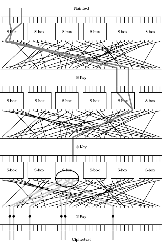
We have a graphical representation of this process of combining S-box characteristics in Figure 7-1. In this diagram, we are using two different relationships (in binary):

(001001 
 011000)
(010010 
 000001)

Both of these characteristics have a probability of 6/64. The first round uses the first characteristic, which has only two output bits affected by the two input bits. These output bits then feed into the second S-box of the second round after permutation.

Each charactistic is expected to be independent of the others; thus, we can multiply the probability of each to obtain a probability for each occurring at the same time:

Note that other S-boxes have no input difference and, therefore, no output difference.

We now have built a characteristic for the entire three-round cipher, starting with two input bits and affecting one intermediate output bit some of the time. We can use this model to derive six of the 18 key bits by selecting a set of plaintext pairs, with their difference being the input differential used to develop the model. Measuring the resulting change in the ciphertext pairs will enable us to find a portion of the key. When the ciphertext pairs yield the expected differential, they form what is called a right pair of plaintext–ciphertexts. (Obviously, plaintext–ciphertext pairs that do not exhibit the desired differentials are called wrong pairs.)

An important addition to the idea of building up characteristics is the idea of an iterative characteristic — one whose input differential is the same as its output differential at some point. These are particularly useful because they can be chained together very easily to create the larger characteristics required for analyzing ciphers with many rounds. I'll show some examples of these when we explore the differential cryptanalysis of DES in Section 7.7.2, although it can apply to any kind of cipher.

Figure 7-1. Differential attack on the EASY1 cipher.

Just as in linear cryptanalysis, we desire to have some number of plaintext– ciphertext pairs to determine the key. However, because differential cryptanalysis is a chosen-plaintext technique, we need to be able to pick certain plaintexts to make the technique work.

Specifically, we pick plaintexts in pairs with differences that are necessary for the characteristic we are testing. In our EASY1 cipher, this difference is Ω_P = 02 80 00 00 00 (bits 30 and 32). We obtain the ciphertexts for both plaintexts and measure the difference in the output. However, in this case, we did not construct the differential characteristic equation to relate the plaintext and the ciphertext: We relate the plaintext to the inputs to the last set of S-boxes. We then brute-force the relevant bits of the key, mix the key bits with the ciphertext, reverse the mixed bits through the S-boxes, and then attempt to perform a match on the output differential. We increment a counter for each key whenever any plaintext/ciphertext pair matches our expected differential.

In general, we expect the correct key to exhibit the probability that we found during analysis. When running the analysis, we obtain Table 7-4 of count values in a sample run.

From Table 7-4, we can note that the largest count is 87, corresponding to the entry for subkey 33 (100001). The key used to generate the ciphertext was 555555555, and we can confirm that the bits of subkey 33 match up correctly with the bits of the key (by looking at how the subkey is mapped to the real key through the permutation, as shown in Figure 7-1).

In total, this technique required approximately 2⁶ × 1000 ≈ 2¹⁶ operations to work. Brute-forcing the remaining bits will take about 2¹² operations, which is not as great as the 2¹⁶ already done. Together, these operations take less time than brute-forcing the 18-bit key (which would take 2¹⁸ operations).

If a full 36-bit key were used, we would have 2³⁰ operations left after the key derivation to brute-force the remaining 30 bits. The 2³⁰ operations in this case would take much longer than the 2¹⁶ operations to derive the 6 bits using differential cryptanalysis; thus, the overall key derivation would still require approximately 2³⁰ operations (less than the 2³⁶ required for brute-forcing a 36-bit key).

The code for implementing differential cryptanalysis, in general, is extremely straightforward. Typically, we do the analysis part offline, where we determine which characteristics to use.

First, we need to perform a simple differential analysis of an S-box. Assume that we have the S-box implemented as a lookup table (in the array s). Listing 7-1 gives us the code to do this, by taking every possible input value for the S-box, calculating the output value, and then measuring, for each input differential possible, the resultant output differential. A table is kept of how many times certain differentials give rise to other differentials.

# The number of bits in the S-box
sbits = 6

# Calculate the maximum value / differential
ssize = 2**6

# Generate the matrix of differences, starting
# at all zeros
count = []
for i in range(ssize):
  count.append([0 for j in range(ssize)])

# Take every possible value for the first plaintext
for x1 in range(0, ssize):
  # Calculate the corresponding ciphertext
  y1 = s[x1]

# Now, for each possible differential

for dx in range(0, ssize):
  # Calculate the other plaintext and ciphertext
  x2 = x1 ^ dx
  y2 = s[x2]

  # Calculate the output differential
  dy = y1 ^ y2

  # Increment the count of the characteristic
  # in the table corresponding to the two
  # differentials
  count[dx][dy] = count[dx][dy] + 1

Next, we show how to generate large numbers of plaintexts and ciphertexts, with the plaintexts having a known differential (see Listing 7-2). This is simply a matter of taking a random plaintext, XORing it with the necessary difference for the differential attack to produce another plaintext, and calculating the relevant ciphertexts to both plaintexts, and storing them. This process is repeated as many times as necessary.

Finally, we perform the differential attack, as shown in Listing 7-3. To perform the differential cryptanalysis, we go through each possible subkey (in this case, there are 64 such subkeys, since it is a 6-bit value). For each of these, we process all of the pairs of ciphertexts (by undoing the last permutation, XORing the subkey in, and going backwards through the appropriate S-box). We then calculate the differential of these processed ciphertexts, and if the differential corresponds to the characteristic we are concerned with, we increment the count of the subkey.

# Import the random library
import random

# Seed it with a fixed value (for repeatability)
random.seed(12345)

# Set the number of rounds in the encryption function
rounds = 3

# Set the number of bits in a plaintext or ciphertext
bits = 36

# Set the plaintext differential
pdiff = 0x280000000L

# Set the number of pairs to generate
numpairs = 1000

# Store the plaintexts and ciphertexts
plaintext1 = []
plaintext2 = []
ciphertext1 = []
ciphertext2 = []

for i in range(0, numpairs):
    # Create a random plaintext
    r = random.randint(0, 2**bits)

    # Create a paired plaintext with a fixed differential
    r2 = r ^ pdiff

    # Save them
    plaintext1.append(r)
    plaintext2.append(r2)

    # Create the associated ciphertexts
    # Assume that the encryption algorithm has already
    # been defined
    c = encrypt(r, rounds)
    c2 = encrypt(r2, rounds)
    ciphertext1.append(c)
    ciphertext2.append(c2)

keys = 64 # number of keys we need to analyze
count = [0 for i in range(keys)] # count for each key
maxcount = −1 # best count found so far
maxkey = −1 # key for the best differential
cdiff = 2# the ciphertext differential we are looking for

# Brute force the subkeys
for k1 in range(0, keys):
  # Adjust the key to match up with the correct S-box
  k = k1 <<18

  # For each p/c pair
  for j in range(numpairs):
    c1 = ciphertext1[j]
    c2 = ciphertext2[j]

# Calculate whatever needs to be done using
  # key bits, storing the results as u1 and u2
  v = mix(demux(apbox(c)), k)
  u = asbox(v[3])

  v2 = mix(demux(apbox(c2)), k)
  u2 = asbox(v2[3])

  # If the differential holds, increment count
  if u1 ^ u2 == cdiff: count[k1] = count[k1] + 1

# If this was the best key so far, then save it
# Otherwise, ignore it for now
if count[k1] >= maxcount:
 maxcount = count[k1]
 maxkey = k1

The sections above introduce the basic concept of differential cryptanalysis on this fairly simple product cipher. However, the concept extends over to Feistel ciphers, the ciphers we are usually most concerned with, quite gracefully.

The first steps are nearly identical: We identify S-box characteristics, and we start tracing those through the cipher. However, the exact way we trace them through the cipher differs somewhat.

Since we have the interaction of the left and right halves, we often have a more difficult task of choosing appropriate characteristics. We often want the differentials to mostly cancel each other out, so that we can control the effects on the next round.

Usually, this is through the use of iterative characteristics. These iterative characteristics will start with a differential. After several rounds through the cipher, they give the same output differential as the input. This enables us to repeat them several times, making analysis very easy. We will see examples of these in the next two sections.

Finally, the last part is key derivation. After the differentials have been traced all the way to the second-to-last round, as before, we then have to ensure that this final differential only modifies the bits of the round function that are affected by some subset of the key bits.

At this point, just as before, we take the two values of the ciphertext and run them through the previous round function. We will be brute-forcing the appropriate key portions of the round functions. The key value that gives us the highest number of the expected characteristics will be our guess.

In the next sections, I'll show how to use these ideas on FEAL and DES.

Differential Cryptanalysis of FEAL

In this section, we will see how the differential cryptanalysis method can be applied to the FEAL block cipher I introduced in Section 4.7. This technique was first presented in Reference [3].

To review, FEAL has a simple DES-like Feistel structure, with an S-box that uses a combination of integer addition, the XOR operation, and bitshifting.

Note, however, that the S-boxes are slightly more complicated than they appear at first glance. They take a 16-bit input and give an 8-bit output. To combat this, consider the middle 16 bits of the f-function, denoted by the equations

f¹ = S(f¹, f², 1)

f² = S(f², f¹, 0)

These can be regarded together as one S-box with a 16-bit input and 16-bit output, since their inputs are the same. The distribution table for this ''super'' S-box has some very interesting properties. Notably, most of the entries (98%) are 0. Furthermore, three of the entries hold with a probability of 1, for example:

(Ω_P = (L || 80 80 80 80))

Some interesting characteristics include iterative characteristics, those in which the input and output XOR differentials are the same. These allow us to construct longer expressions with less complicated analysis. For example, in FEAL, the following is a four-round iterative characteristic that holds with probability 2⁻8:

(Ω_P = 80 60 80 00 80 60 80 00)

Differential Cryptanalysis of DES

At the time when differential cryptanalysis was developed, DES was in widespread use and was often the target of many new techniques. The use of differential cryptanalysis against DES was first presented in Reference [2], as one of the first uses of differential cryptanalysis, and with surprising results (see Table 7-5).

Table 7-5. Differential Cryptanalysis Attack Against DES: Complexities for Different Numbers of Rounds [2]

ROUNDS	COMPLEXITY OF ATTACK
4	24
6	28
8	216
9	226
10	235
11	236
12	243
13	244
14	251
15	252
16 (full DES)	258

To start off, I'll show how to break the three-round DES, and then extrapolate the process further.

For our plaintext differential, we will always have the right (least significant) 32 bits be all zeros, with the left (most significant) being a particular pattern.

Recall from Chapter 4 that DES's main round function looks as follows:

1. R_i+1 = L_i ⊕ f (R_i, K_i+1).

2. L_i+1 = R_i.

Expanding this out to three rounds (values in bold are known values):

1. R₀ = 0.

2. L₀ (arbitrary, random).

3. R₁ = L₀ ⊕ f (0, K₁).

4. L₁ = R₀ = 0.

5. R₂ = L₁ ⊕ f (R₁, K₂) = f (R₁, K₂).

6. L₂ = R₁.

7. R₃ = L₂ ⊕ f (R₂, K₃) = R₁ ⊕ f (R₂, K₃).

8. L₃ = R₂ = f (R₁, K₂).

Now, if we have a second plaintext-ciphertext pair (say, L′₀, R′₀, L′₃, R′₃), with the new plaintext having a known differential to the previous plaintext (Ω), then we have the following derivation:

1. R′₀ = 0 (= R₀).

2. L′₀ = L₀ ⊕ Ω (arbitrary, random).

3. R′₁ = L′₀ ⊕ f (0, K₁) = R₁ ⊕ Ω.

4. L′₁ = R′₀ = 0.

5. R′₂ = L′₁ ⊕ f (R′₁, K₂) = f (R₁ ⊕ Ω, K₂).

6. L′₂ = R′₁.

7. R′₃ = L′₂ ⊕ f (R′₂, K₃) = R′₁ ⊕ f (R′₂, K₃).

8. L′₃ = R′₂ = f (R₁ ⊕ Ω, K₂).

Here, we have underlined where the differential propagates.

From the last steps of the two previous lists, since we know the values of L₃ and L′₃, we can calculate Δ, the difference in the ciphertexts. We also can perform a differential analysis of the S-boxes of DES, so that the effect of the differential Ω would be known, and we can choose Ω to exploit this for each S-box (since DES has several distinct S-boxes).

Once we know some good characteristics of the round function, we can then set up the three-round cipher to use the plaintext differential on the left to create differences in the plaintext. After measuring enough of these, we will be able to make good guesses at the key bits.

In general, we can easily see that if the right-half XOR is 0, and the left half has an arbitrary differential (say, L), we can construct a characteristic for a round of DES.

First, as shown above, if the input to the round function (f) is the same(with a zero XOR), then the output is the same. The new left half in both cases is the old right half (which is the same, since there is a zero XOR). The new right half is the XOR of the round function value (which is the same) and the old left half, which has a differential of Ω_L. The characteristic can be written as

((Ω_L || 0)

Furthermore, there is no guessing in this; thus, this characteristic has a probability of 1.

Let's construct another good characteristic. Again, assuming a constant differential for the left half (Ω_L), if we consider the right half having the differential 60 00 00 00, then the input to the round function will also have that same XOR. Using S-box analysis, we can show that the output differential of the round function 00 80 82 00 occurs with probability 14/64.

This differential would then be XORed with the previous differential (Ω_L), to obtain the following one-round characteristic:

((Ω_L 60 00 00 00)

Now that we have these two characteristics, we can combine them to create a fairly good three-round characteristic. To see how this is done, simply look at the previous characteristic, and assume that Ω_L = 00 80 82 00.

In this case, we will have the following chain, using the second, first, and second characteristics in that order:

(00 80 82 00 || 60 00 00 00)
 (60 00 00 00 || 00 00 00 00)
 (00 00 00 00 || 60 00 00 00)
 (00 80 82 00 || 60 00 00 00)

This is an example of an iterative characteristic: It yields itself after several rounds. Therefore, these can be chained together to create larger and larger characteristics.

Cryptanalysis of DES itself using this characteristic, as well as a few others, gives us an approximation for enough of the cipher to start brute-forcing particular subkey bits.

Now that we have seen exactly how to perform differential cryptanalysis, it's fair that we should attempt to analyze its operations and discuss some of its properties.

As we have shown, differential cryptanalysis has two primary features: It is a probabilistic attack, and it is a chosen-plaintext attack. Neither of these scenarios is ideal, but we are stuck with them.

The implications of this probabilistic attack are similar to the properties of other probabilistic problems. We aren't guaranteed to get good results, even with perfectly good inputs and a sufficient number of chosen plaintexts. The more chosen plaintexts we do have, however, the more likely we are to succeed.

Another disadvantage of this method is that we will come up with an answer no matter what; the answer will just be incorrect if we don't have a sufficient number of texts to test it against. Furthermore, there is no way to tell if the key bits derived are correct until we derive all the rest of the key bits and actually test encrypting the plaintext with the potential key (unless we know the answer ahead of time).

The fact that this algorithm is chosen plaintext is another step back: Chosen plaintexts represent some of the most stringent conditions of a cryptanalytic attack. They require the cryptanalyst to not only know and understand the cryptographic algorithm being used, have developed a plan of action against it, and collected a large amount of ciphertext with known plaintext values, but in addition have the ability to manipulate this plaintext! This is a fairly tall order and is a bit less practical than a known-plaintext attack or a ciphertext-only attack.

Finally, we have the fact that to execute the attack at all, we must store a large number of plaintext–ciphertext pairs. There are ways around this, in test scenarios at least, where we reverse the order that we do things. We first generate a new plaintext–ciphertext pair, XOR the plaintext to obtain the resultant ciphertext, and then try every possible subkey against it, incrementing their respective counts, as necessary. At the end of this computation, we can throw away the pairs and generate new ones. Thus, in some cases, we can mitigate this storage problem.

Moreover, the improvements in time over exhaustive search represent a tremendous breakthrough, even considering the strenuous requirements to implement the improvements.

Although differential cryptanalysis has several drawbacks, the overall concept has had a powerful impact on cryptanalysis. In the following sections, we examine some of the fundamental extensions of differential cryptanalysis.

An interesting combination of the two important algorithms presented in the last two chapters, linear and differential cryptanalysis, appeared in Reference [12], courtesy of Susan Langford and Martin Hellman.

The trick is to use a linear expression, developed in the way already shown, and to measure what changes in the plaintext do to the value of that linear expression. In this way, we aren't simply brute-forcing the subkey by calculating counts on the linear expression; rather, we are using carefully selected differentials that should produce fixed, expected probabilities of the two linear expressions being XORed being equal to 0. As before, we normally expect this to happen roughly half the time for any arbitrary linear expression and difference; thus, any deviation from this can be used.

A good example that the authors show is using a three-round linear approximation for DES. A normal linear expression proposed by Matsui is

This holds with a probability of either approximately 0.695 or 0.305.

The differential attack comes from noting that we can toggle bits 29 or 30 (or both) of the L₁ value, and this will produce no changes in the fourth-round linear approximation. This means, at this point, that our linear approximations XORed together have a probability of 1 of occurring.

Carrying this out to an eight-round approximation, the probability of the linear expression XOR becomes

0.695² + 0.305² = 0.576

We add the numbers together since we could either be right twice in a row or wrong with our expression twice in a row, and we can't really tell the difference. As the authors of the paper say, two wrongs make a right in binary arithmetic.

This means we have a bias of 0.076, giving us an approximate number of plaintext–ciphertext pairs:

8 × (0.076)⁻² ≈ 1400

We can even pull another trick to reduce this number further.

Since we still have to get bits 29 and 30 to toggle in L₁, we will naturally have to toggle bits in the plaintext (L₀ and R₀). Toggling the same two bits in R₀ will perform this.

We will also toggle bits 1, 9, 15, and 23 of L₀: These are the output bits of the S-box S₁ (which is also affected by 6 bits of the key). Bits 29 and 30 arealso used as the input to S₁ (and no other S-box in round 1); thus, our changes affect only S₁. This gives a total of 64 plaintexts, with their ciphertexts.

At first glance, none of these plaintext–ciphertext pairs are really "paired" in the way that differential cryptanalysis requires. However, it turns out that there are several such pairings. We can pair each plaintext value (there are 64) with three other plaintexts: one with bit 29 of R₀ toggled, one with bit 30 of R₀ toggled, and one with both bits toggled in R₀. This way, we have three pairs, for a theoretical total of 64 × 3 = 192 pairings. In reality, we get half as many (96), since half of the pairings are redundant.

This way, we are getting 96 pairings for 64 plaintexts (a ratio of 3-for-2), instead of the normal 1-for-2 of standard differential cryptanalysis because in differential cryptanalysis, we generate one plaintext, and then XOR it with a fixed value to obtain another plaintext. Thus, we have two plaintexts and one pairing, for a ratio of 1-for-2, which is approximately three times less efficient than combining the two techniques.

While this technique doesn't yield more key bits than either differential or linear cryptanalysis, it does allow us to derive these key bits with fewer plaintext–ciphertext pairs, while still maintaining a high success rate. There are some issues with scalability, though: This method works well for fewer numbers around and doesn't apply well to more rounds.

It is difficult to apply differential cryptanalysis to certain classes of ciphers. For example, if we have certain portions of the cipher modify the structure of the cipher itself based on the key, then we would not be able to effectively develop iterative characteristics to use in differential cryptanalysis. Ben-Aroya and Biham explore a particular method against two particular ciphers thought to be strong against differential cryptanalysis using a technique called conditional characteristics [1].

One of the ciphers they analyze is called Randomized DES (RDES). Many cryptologists thought that a way to limit the susceptibility of DES to differential cryptanalysis was to swap the left and right halves during some of the rounds: which rounds depended on the key value. Since there are 16 different rounds, there would be 2¹⁶ = 65,536 different combinations of swapping and not swapping, thereby making normal differential analysis extremely difficult.

Naturally, there is one problem. For a certain number of keys (one out of every 2¹⁵ of them), there would be no swapping at all! If subjected to a known-plaintext attack, the entire right half would not be affected by the encryption, passing through the rounds untouched. Similarly, for another set of one out of every 2¹⁵ keys, there would only be a swap on the last round, allowing us to easily derive most of the key bits using simple analysis of the inputs and outputs of the round function.

The rest of the keys is where the concept of a conditional characteristic comes in handy. A conditional characteristic is a characteristic that is dependent on the key being used. Typically, the characteristic is only effective against keys with certain properties (such as certain bits being set). The number of keys that the conditional characteristic is good for, divided by the total number of keys, is called the key ratio.

The attack uses two different round function characteristics of DES:

(0

(19 60 00 00

When combined, they provide a two-round iterative characteristic:

((19 60 00 00 00 00 00 00)

In DES, we can iterate this characteristic many times, but owing to the swapping and non-swapping portions of RDES, we can't use this one as is.

We can, though, use the individual components. Essentially, we use the first characteristic (0

We can produce a second characteristic for the entire cipher in a very similar way, only starting with the second round characteristic in the first round, and then using the first round characteristic after the first swap, and alternating to fill the rest of the cipher (using a new characteristic for each swap).

At least one of these characteristics will have a probability of (1/234)^r, where r is the number of rounds of the characteristic (or, equivalently, the number of swaps).

In this way, we will have to produce characteristics for all of the 2¹⁵ possible swapping scenarios. However, we have only two characteristics per swapping scenario, requiring us to have only about twice as many chosen plaintext–ciphertext pairs as normal differential cryptanalysis.

But the advantage is, if there are less than 13 swaps, then the probability will be much greater than the normal DES probability, decreasing the cost of the attack. At 13 swaps, the complexity of the attack is 2⁴⁶. It turns out that 98 percent of the keys will generate 13 swaps or less. Since this leaves only 1/50 keys left, we can do an exhaustive search of these if the above attack fails, leaving only a 2⁵⁰ attack, which is still better than DES.

Therefore, using conditional characteristics, we have proved that the security of RDES is always less than DES, and in many cases, is significantly worse.

Differential cryptanalysis is the study of normal differentials, where we have two texts, X₁ and X₂, and we use information about the difference of those two texts:

Ω_X = X₁ ⊕ X₂

This difference allows us to analyze how the cipher changes.

There was some effort to start arming ciphers to become immune to these differential attacks, for example, by using S-boxes with more uniform differences, as well as other techniques [10, 15].

One of the responses to this trend is the concept of higher-order differentials [9, 11]. If we have a difference of plaintexts, for example, why stop at just this one difference? Why not have a difference of the difference of the plaintexts, and see if we can use this to determine any information? This would be a second-order differential. We can also have third-order, fourth-order, and so forth.

More formally, suppose that we have a differential, Ω_X, and another differential, Ω′_X. We can define a second-order input differential, say,

This requires us to have four ciphertexts, say, X₁, X₂, X₃, and X₄, such that the first-order differentials are

Then the second-order input differential is

However, the output differential (of F, which could be a round function, or one or more rounds) is normally referred to as the second-order differential. For the first-order output differentials, we would then have

And for the second-order output differential:

This would give us the second-order characteristic:

I use the symbol ''

This process can be extended further to create higher-order differentials. Formally, for these, we can use a slightly different notation from Reference [9], as the above notation can quickly become a bit cumbersome. Furthermore, the above notation applies only to standard binary ciphers. For ones that take place, for example, in finite fields, we need a slightly different notation, since the operation to take the difference might be different from the one to add a difference.

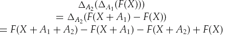
Let a first-order differential of the output of a round function F of an input point X be denoted

where A₁ is the differential of the input. For a second-order differential, we have

We'll expand this so it is a little clearer:

This technique of higher-order differentials can be very useful. In Reference [9], Knudsen shows that the round function f (x +k)² mod p, where p is prime (and has a block size of twice the number of bits in p), has no useful first-order differentials. However, if we use second-order differentials, we can break the round function very easily.

In standard differential cryptanalysis, we take a fixed difference in the input and rely on this difference producing a chain reaction of a step-by-step series of differences, which eventually trickle down to a point that we can measure. When we measure at this point, we are looking for an exact difference between two ciphertexts: We count these exact differences, and ignore any plaintext–ciphertexts pairs that do not have this difference in the ciphertext.

To be more specific, in the above standard differential attacks, we would check to see if there was a difference by XORing the two values and checking the value of the output. If it matched what we expected, then it's a hit. Otherwise, it's not, even if all of the bits we expected to be flipped were, but some extra bits were also flipped.

The concept of truncated differentials relaxes the constraint that we need to look for the entire difference to be exactly what we use (in the input difference) or what we predict (in the output difference). If we have a normal characteristic, with two differentials:

(Ω_X

then we have a truncated differential:

(Ω′_X

where Ω′_X and Ω′_Y, respectively, represent subsets of the differentials Ω_X and Ω_Y. Theterm subsets here means that just some (or possibly all) of the bits that are different in characteristics will be different in the truncated differential.

For example, DES itself has known truncated round characteristics of probability 1.

Knudsen in Reference [9] gives a simple attack on a five-round Feistel cipher with an n-bit round function (and, therefore, a 2n-bit block size). Let the Feistel round function be F. Assume we have a non-zero input truncated differential Ω_a, using only some of the bits:

This will generate a list of keys proportional to the number of key bits in the truncated differential. Repeating this a sufficient number of times, we will have only a single set of keys come out each time.

We can use this same attack on any number of rounds by doing the exact same analysis, except for the first three rounds. Naturally, with each application, we have to do more work and will have less precision.

Truncated differential analysis is a potentially powerful technique. It has been done on the Twofish Algorithm [17] in Reference [14], although it has not been used in a successful attack as yet [16].

Impossible differentials were used successfully to cryptanalyze most of Skipjack [19] (31 out of 32 rounds) by Biham, Biryukov, and Shamir [4].

The idea is fairly simple: Instead of looking for outcomes that are as highly probable as possible, we look for events that cannot occur in the ciphertext. This means that, if we have a candidate key (or set of key bits) that produces a differential with a probability of 0, then that candidate is invalid. If we invalidate enough of the keys, then we will be left with a number reasonable enough to work with.

As Biham et al. [4] point out, events that should be impossible have been historically used in other events [5]. For example, with a German Enigma machine, it was not possible for any plaintext character to be encrypted to itself. Therefore, any potential solution of a ciphertext must not have a character of plaintext be the same as the corresponding character in the ciphertext.

The particular attack Biham et al. [4] explain is a miss-in-the-middle attack on Skipjack. If we feed an input differential into round 5 of (0, a, 0, 0)[into(w₅, w₆, w₇, w₈)], then we can check for an impossible output differential in (the output of) round 28: (b, 0, 0, 0). We will write this impossible differential as

This differential is impossible if a and b are both not 0. (The rounds are numbered from 1 to 32.)

This is a miss-in-the-middle attack because, if we analyze the differentials from round 5 and round 28, we can trace them all the way to the output of round 16 (or, equivalently, the input of round 17); two effects of each differential meet: The input differential says that the round value should be (c, d, e, 0), while the output differential says that the round value should be (f, g, 0, h). Specifically, e and h cannot be 0, and therefore there is a contradiction. Figure 7-2 graphically depicts the impossible differential attack.

For the exact details of the full attack, including complete details on a key recovery attack, see Reference [4]. However, I'll outline the attack below.

This technique can be used to derive a key in the following way. We use the above differential

The above key recovery attack, unfortunately, only seems to work for up to about 26 rounds of the full 32-round Skipjack. With 31 rounds, Biham et al. [4] instead found that they would have to check every single key. Luckily, checking every single key does not require performing the complete encryption or decryption: It can be limited to a handful of computations of the G-function. Since a full encryption works by using several G-function computations, as long as we keep the number of G computations down below the amount required for a full encryption, we are still doing less work than would be required on a normal exhaustive attack. The authors predict about 2⁷⁸ steps, with 2⁶⁴ bits of memory (2,048 petabytes). This is still faster than an exhaustive attack, which would require 2⁸⁰ steps.

One of the most important contributions of the concept of impossible differentials is that the normal method of ''proving'' cipher secure against differential cryptanalysis — that by creating a very low upper bound on probabilities of differentials in the components — is flawed. If there are a sufficient number of zero or low-probability differentials, then the impossible differential attack can be carried out.

Furthermore, this same attack can be applied with conditional characteristics and differentials, as well as linear cryptanalysis.

Figure 7-2. A graphical depiction of the impossible differential attack on Skipjack, based on a diagram from Reference [4]. The rounds have been ''unrolled'' from the shift register mechanism, allowing us to more easily see the mechanism. We can see the differentials missing in the zero, as one side predicts a zero, and the other side predicts a non-zero intermediate.

So far, we have been focusing almost entirely on top-down approaches to cryptanalysis: Our attacks work by taking information about the plaintext, and deriving some feature of the ciphertext that we will test. How often the test succeeds gives us a likelihood that a key is correct.

The above attack with impossible differentials, as well as the previously discussed meet-in-the-middle attack, shows us that this view may be missing out on some advantages to working both ends at once. Linear cryptanalysis even uses some of this symmetry to help derive more key bits.

The boomerang attack is another differential meet-in-the-middle attack [20].

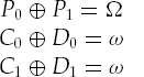
The basic premise uses four pairs of plaintexts and their associated ciphertexts:

(P₀, C₀), (P₁, C₁), (Q₀, D₀), (Q₁, D₁)

Using the premises of Reference [20], let's break the encryption operation (E) into two subparts:E₀ (the first half of the encryption) and E₁ (the second half of the encryption). For example:

C₀ = E (P₀) = E₁(E₀(P₀))

I'll denote the inverse operations of E₀ and E₁, as in, the decryption operations, as

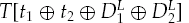
Here, we will have to develop two characteristics, one for the first half of the encryption, E₀, and one for the second half's decryption,

Note that the

Using these two characteristics, we can then derive a new characteristic for the intermediate encryption of Q₀ and Q₁:

Figure 7-3. Derivation of the boomerang differential P₀ ⊕ P₁ = Ω leading to Q₀ ⊕ Q₁ = Ω, based on a diagram in Reference [20]. (Light gray lines) XOR's; (dark gray lines) how the differentials propagate from the P's to the Q's; (black lines) encryption.

Hence, we have derived a new characteristic for the Q values:

This characteristic can then be measured by calculating Q₀ ⊕ Q₁ = Ω. Figure 7-3 shows a graphical representation of how this characteristic occurs.

From the diagram and the derivation above, we can see why this is called the boomerang attack: If we construct the differentials correctly, the differential Ω will come back and hit us in Q₀ ⊕ Q₁.

We construct the boomerang differential by taking a seed plaintext P₀ with our Ω differential and creating P₁ = P₀ ⊕ Ω. We then encrypt P₀ and P₁ to obtain C₀ and C₁, respectively. Next, we calculate new ciphertexts with our ω differential, so that D₀ = C₀ ⊕ ω and D₁ = C₁ ⊕ ω. We then decrypt D₀ and D₁to obtain Q₀ and Q₁. Some percentage of the time, the moons will align and the differentials will all line up, allowing us to measure to see if Q₀ ⊕ Q₁ = Ω. When all four differentials hold, we refer to this as a right quartet.

What is the significance of this attack? Well, many algorithms have been deemed to be ''secure'' against differential cryptanalysis because of the lack of any good characteristics on the full cipher. Normally, as the number of rounds increases, the probability of the differential decreases, thereby requiring more and more plaintext–ciphertext pairs.

The above boomerang attack lets us develop an attack using only the characteristic for the first half of the cipher, bypassing the latter half. If sufficiently strong characteristics exist, then we have a good attack. We use the characteristics just as before to derive the key. With the characteristic properly set in the final (and first) rounds, we can brute-force the keys that affect the differential, measure it, and select the most likely candidate key bits.

After this first layer is stripped away, we can continue developing characteristics to get more key bits, or just perform an exhaustive search on the remaining key bits.

Wagner [20] uses exactly this premise against the COCONUT98 algorithm [18]. COCONUT98 has a 256-bit key and was developed specifically to defeat differential cryptanalysis by having no useful characteristics. Despite this, COCONUT98's key can be derived using the boomerang attack with 2¹⁶ chosen plaintext–ciphertext sets, with 2⁴¹ offline computations (equivalent to 2³⁸ encryptions, according to Reference [20]).

In addition to its attack on COCONUT98, Reference [20] also mounts an incredibly successful attack against FEAL (Section 4.7) and Khufu, a 64-bit block cipher with a 512-bit key [13].

Many of these differential techniques are extensions of standard, continuous techniques of calculus, such as the derivative. As a matter of fact, differentials are sometimes referred to as derivatives. The primary difference is that, instead of applying the techniques to continuous spaces, like real or complex numbers, we are applying the techniques to discrete spaces — in our case, integers between 0 and 2ⁿ.

Another technique many learn is interpolation: If we wish to find a line between two points, or a parabola between three, or, in general, a polynomial of degree n − 1 that passes between n points, there is a simple formula to calculate this polynomial. These formulas can be used to analyze the relationship between various points or to find additional points lying in between points.

For example, for a simple line between two points (x₀, y₀) and (x₁, y₁) we can see that the following line includes both points:

If we plug in x₀, weget y₀, and if we plug in x₁, we get y₁. The function is linear because it contains only the variable x.

In the general case, for points (x_i, y_i), for i = 1, ..., n, our interpolating polynomial, p (x), is given by

This is merely an extension of our previous case to produce a polynomial of degree n − 1. This is called the Lagrange interpolating polynomial.

This technique can also be applied to the discrete world of bits and bytes, as shown by Jakobsen and Knudsen [7]. We simply apply the above definitions to discrete functions, where the x- and y-values will be plaintext and their associated ciphertexts, respectively.

We can apply this technique by noting that 32-bit XOR operations are identical to algebraic addition in the finite field GF (2³²) (since it has characteristic 2, i.e., 2 is equivalent to 0, so that 1 + 1 = 0).

Constructing this polynomial will not immediately yield the key, however. Given sufficient pairs, it can actually yield a polynomial that emulates the encryption function: It produces valid ciphertexts from given plaintexts.

To actually get key bits, we instead try to find a polynomial for the plaintext and the next-to-last round of ciphertext. Similar to the way we have done before, we decrypt some portion of the last round by guessing the last round key. When we have done this for a sufficient number of plaintext–ciphertext pairs, we will have enough plaintext and intermediate ciphertext pairs to attempt to construct a polynomial. We check the polynomial against another value that wasn't used in the construction to test it. If the polynomial produces the correct result, then we have guessed the key bits.

The interpolating attack is a bit academic in nature, but it provides an interesting avenue of attack. For certain ciphers that provably secure against traditional differential cryptanalysis, the interpolating attack produces a very reasonable method for deriving the key, as shown in Reference [7].

Finally, we want to look at a completely different way of viewing differential cryptanalysis. In the previous sections, we analyzed ciphers by examining how differences in the plaintexts and ciphertexts propagate to determine key bits. This was accomplished through the use of chosen-plaintext attacks.

One avenue unexplored is that of attacking the key itself. After all, we have considered the key to be out-of-bounds for modifications. It hasn't been part of our model to modify it, since it is what we are trying to derive. Furthermore, doesn't the ability to change the key automatically mean that we know the value of it?

Actually, no. As Kelsey, Schneier, and Wagner [8] point out, many key exchange protocols leave themselves vulnerable in two ways. The first way is that they do not check the integrity of the key before they start using it to encrypt plaintext into ciphertext encrypted — meaning that, immediately after exchanging the keys, they immediately encrypt some plaintext and send the ciphertext to the other party.

Secondly, many key exchange protocols use simple XOR structures to pass along the key. For example, assume that there is a pre-shared secret key, K_m. A new session key may be generated by sending a message:

(M, E_Km (M) ⊕ K_s)

This two-part message will hide the actual value of the key. However, if we have the ability to modify the message in transit, then we could corrupt the key the first time around with a known difference. Now, one party will send a message encrypted with one key, and the other will send a message encrypted with the key XORed with a fixed, chosen difference.

Typically, we also address this attack as a chosen plaintext, so that both parties would attempt to encrypt the same plaintext with the XORed keys.

Owing to the difficulty of achieving such an attack, this scenario has often been disregarded. However, the above key-exchange scenario should provide some conjecture that the above attack is very possible.

Naturally, the XOR difference will have to be significant, usually to exploit a weakness in the key-scheduling algorithm. Attacks that rely on such weaknesses are called related-key attacks, since the attack relies on so-called ''related keys'' in the schedule. Indeed, many ciphers use schedules in which key bits are copied or have a linear relationship to many other bits.

Related-Key Attack on GOST

Sometimes the related-key attack can be carried out with a normal differential attack. In Reference [8], the authors exploit a key scheduling weakness in the GOST 28147-89 cipher, a Soviet cryptosystem [6]. The key schedule they specify takes a 256-bit key and breaks it into eight 32-bit subkeys, K₀, ..., K₇, generating subkeys (sk_i) for use in the 32 rounds by

We can use this key schedule in a clever manner.

Say that we have an interesting differential for the plaintext on this algorithm, Ω. Since the keys (in most ciphers, actually) are directly XORed in at some point, we should be able to choose a related key to the original that will counteract the Ω for the first round. This could be done simply by taking K₀ = K₀ ⊕ Δ, for some appropriate value of Δ.

Note that the subkeys for the next seven rounds (i = 1, ..., 7) don't rely on K₀. This means that the difference for each of these rounds from the original plaintext is zero! The differences will then start with the eighth round. In essence, we skipped the first eight rounds of the cipher and can instead mount a much simpler 24-round attack.

Related-Key Attack on 3DES

A very interesting use of a related-key attack is on 3DES, using three separate keys [8]. We recall that 3DES uses the standard DES encryption function three times in succession, each time with a different key. (The decryption, naturally, decrypts with the keys in the exact opposite fashion.) This allows us to virtually triple the total key space, while not changing the underlying structure of DES at all.

Assume that we have a DES encryption of a plaintext P to a ciphertext C, using keys K_a, K_b, and K_c as follows. Let the E-function represent DES encryption, and the D-function represent DES decryption. Then,

Now, assume that we have a related key, with K′_a = K_a ⊕ Δ. We select to have the original C decrypted to give us a new plaintext, P′, or

Note that the decryption to P is

That is, the decryption to P and P′ differs only in the last step, allowing us to write

We can then treat this as a known-plaintext attack and attack it via an exhaustive search, for 2⁵⁶ work, deriving K_a in the process.

Once we have K_a, we can then obtain E_Ka(P), allowing us to look at it, along with C, as a known plaintext–ciphertext pair of double DES. We may recall that double DES is susceptible to a meet-in-the-middle attack with 2⁵⁷ work.

With a related-key attack, we have then broken 3DES to be no better than normal DES. Note, however, that this works only when all three keys are independent. The most common form of 3DES, with the first and third keys the same, is immune to this attack, as the differential would carry into the first and last steps of both encryption and decryption.

Finally, the authors of Reference [8] give some guidance on how to avoid related-key attacks.

First, avoid using key-exchange algorithms that do not have key integrity; always check the key before using it blindly to encrypt something and broadcasting it.

Second, making efforts to not derive round keys in such linear manners will go a long way. The authors make a very good suggestion of running the key first through a cryptographic hash function, such as SHA-1, and then using it to derive a key schedule. Any sufficiently strong hash function will obliterate any structures that may have been artificially induced, preventing them from meaningfully modifying the ciphertext.

In this chapter, I demonstrated many modern differential attacks against modern ciphers. The standard differential attack has been extended and studied extensively over the past two decades and continues to be in conferences and papers every year.

There is always more to learn in the field of cryptanalysis. This book only covered some of the more popular and influential topics in the field. To the reader wanting to learn even more about the field, you can look through the archives and current issues of The Journal of Cryptology, Cryptologia, the proceedings of conferences such as CRYPTO, EUROCRYPT, ASIACRYPT, Fast Software Encryption, and many others.

Again, we must reiterate, though: The best way to become a better cryptanalyst is to practice, practice, practice!

Exercise 1. Change the S-box and P-box of the EASY1 cipher to randomly generated values. Use the analysis in this chapter to create a differential attack on this for three rounds.

Exercise 2. Use the basic one-round version of the cipher from the previous exercise as a round function to a simple Feistel cipher. Use a simple key schedule, such as using the same 36-bit key every round.

Use differential cryptanalysis to break this Feistel cipher for eight rounds. Give analysis for how many plaintext–ciphertext pairs this will require.

Exercise 3. Perform a differential analysis of the S-boxes of DES. Discuss your results.

Exercise 4. Perform a differential analysis of AES. How successful would you guess a standard differential attack against AES might be based on this analysis?

Exercise 5. Attempt an impossible cryptanalysis attack against the cipher you created in Exercise 1. Try again with the Feistel cipher in Exercise 2.

Exercise 6. Mount a boomerang attack against the cipher you created in Exercise 2, but extend the number of rounds to 16.

References

^[92]

^[93]

^[94]

^[95]

^[96]

^[97]

^[98]

^[99]

^[100]

^[101]

^[102]

^[103]

^[104]

^[105]

^[106]

^[107]

^[108]

^[109]

^[110]

^[111]

References

[92] [1] I. Ben Aroya and E. Biham. Differential cryptanalysis of lucifer. In Advances in Cryptology – Crypto '93, (ed. Douglas R. Stinson), pp. 187–199. Lecture Notes in Computer Science, Vol. 773. (Springer-Verlag, Berlin, 1993).
[93] [2] E. Biham and A. Shamir. Differential cryptanalysis of DES-like cryptosystems (extended abstract). In Advances in Cryptology – Crypto '90, (eds. Alfred J. Menezes and Scott A. Vanstone), pp. 2–21. Lecture Notes in Computer Science, Vol. 537. (Springer-Verlag, Berlin, 1990).
[94] [3] E. Biham and A. Shamir. Differential cryptanalysis of Feal and N-hash. In Advances in Cryptology – EuroCrypt '91, (ed. Donald W. Davies), pp. 1–16. Lecture Notes in Computer Science, Vol. 547. (Springer-Verlag, Berlin, 1991).
[95] [4] Eli Biham, Alex Biryukov, and Adi Shamir. Cryptanalysis of skipjack reduced to 31 rounds using impossible differentials. Journal of Cryptology 18 (4): 291–311 (2005).
[96] [5] Cipher A. Deavours and Louis Kruh.Machine Cryptography and Modern Cryptanalysis, Artech House Telecom Library. (Artech House Publishers, Norwood, MA, 1985).
[97] [6] Government Standard 28147-89. (Government of the USSR for Standards, 1989).
[98] [7] Thomas Jakobsen and Lars R. Knudsen. The interpolation attack on block ciphers. In Fast Software Encryption: 4th Interntional Workshop, FSE '97, (ed. Eli Biham), Lecture Notes in Computer Science, pp. 28–40. Lecture Notes in Computer Science, Vol. 1267. (Springer-Verlag, Berlin, 1997); http://citeseer.ist.psu.edu/jakobsen97interpolation.html.
[99] [8] J. Kelsey, B. Schneier, and D. Wagner. Key-schedule cryptanalysis of IDEA, G-DES, GOST, SAFER, and triple-DES. In Advances in Cryptology – Crypto '96, (ed. Neal Koblitz), pp. 237–251. Lecture Notes in Computer Science, Vol. 1109. (Springer-Verlag, Berlin, 1996).
[100] [9] Lars R. Knudsen. Truncated and higher order differentials. In Fast Software Encryption: Second International Workshop, Leuven, Belgium, December 14–16, 1994, (ed. Bart Preneel), pp. 196–211. Lecture Notes in Computer Science, Vol. 1008. (Springer-Verlag, Berlin, 1995); http://iteseer.ist.psu.edu/knudsen95truncated.html.
[101] [10] Kenji Koyama and Routo Terada. How to strengthen des-like cryptosystems against differential cryptanalysis.IEICE Transactions on Fundamentals of Electronics Communications and Computer Sciences E76-A (1): 63–69 (1993).
[102] [11] Xuejia Lai. Higher order derivatives and differential cryptanalysis. In Proceedings of Symposium on Communication, Coding and Cryptography (Monte-Vina, Ascona, Switzerland, 1994).
[103] [12] S. K. Langford and M. E. Hellman. Differential-linear cryptanalysis. In Advances in Cryptology – Crypto '94, (ed. Yvo Desmedt), pp. 17–25. Lecture Notes in Computer Science, Vol. 839. (Springer-Verlag, Berlin, 1994).
[104] [13] R. C. Merkle. Fast software encryption functions. In Advances in Cryptology – Crypto '90, (eds. Alfred J. Menezes and Scott A. Vanstone), pp. 476–501. Lecture Notes in Computer Science, Vol. 537. (Springer-Verlag, Berlin, 1990).
[105] [14] Shiho Moriai and Yiqun Lisa Yin.Cryptanalysis of Twofish (II); http://www.schneier.com/twofish-analysis-shiho.pdf.
[106] [15] K. Nyberg and L. R. Knudsen. Provable security against differential cryptanalysis. In Advances in Cryptology – Crypto '92, (ed. Ernest F. Brickell), pp. 566–574. Lecture Notes in Computer Science, Vol. 740. (Springer-Verlag, Berlin, 1992).
[107] [16] Bruce Schneier.Twofish Cryptanalysis Rumors. (2005); http://www.schneier.com/blog/archives/2005/11/twofish cryptan.html.
[108] [17] Bruce Schneier, John Kelsey, Doug Whiting, David Wagner, Chris Hall, and Niels Ferguson.The Twofish Encryption Algorithm: A 128-Bit Block Cipher. (John Wiley, New York, 1999).
[109] [18] S. Vaudenay. Provable security for block ciphers by decorrelation. In STACS 98: 15th Annual Symposium on Theoretical Aspects of Computer Science, Paris, France, February 25–27, 1998, Proceedings, (eds. Michel Morvan, Christoph Meniel, and Daniel Krob). Lecture Notes in Computer Science, Vol. 1373. (Springer-Verlag, Berlin, 1998).
[110] [19] U.S. Government.SKIPJACK and KEA Algorithm Specifications. (1998).
[111] [20] David Wagner. The boomerang attack. In Fast Software Encryption: 6th Interntional Workshop, FSE '99, (ed. Lars R. Knudsen), pp. 156–170. Lecture Notes in Computer Science, Vol. 1636. (Springer-Verlag, Berlin, 1999); http://citeseer.ist.psu.edu/wagner99boomerang.html.