There is another important notion in understanding algorithms: writing them out clearly, and unambiguously. For doing so, authors typically take one of three approaches: picking a programming language du jour to write all examples in, inventing a programming language, or writing everything in various forms of pseudocode (writing out the instructions in some mesh of natural language and a more formal programming language).

The first approach, picking a popular or well-known language, has an obvious disadvantage in that it dates a book immediately: a book written 40 years ago might have used FORTRAN or ALGOL to implement its algorithms, which would be difficult for many readers to understand. The second approach can be all right, but it requires that the reader learn some language that the author thinks is best. This approach can have mixed results, with some readers distracted so much by learning the language that they do not comprehend the text.

The final approach is often used, especially in abstract books. While usually very clear, it can sometimes be a challenge for a programmer to implement, especially if important details are glossed over.

The approach we use in this book is to have a combination of pseudocode and writing out in an actual programming language. The pseudocode in this and the following chapters is very simple: I merely state how a program would operate, but in mostly plain English, instead of some abstract notation. The intent of this book is not to alienate readers, but to enlighten.

For some examples, I will like a reader to be able to easily see an algorithm in action and to have some kind of source code to analyze and run. When these situations arise, I implement in a language that, in my opinion, has a complete, free version available over the Internet; is easy to read even if the reader is not fluent in the language; and in which the reader won't get bogged down in housekeeping details (like #include <stdio.h>-like statements in C, import java.util.*; statements in Java, etc.). A few languages fulfill these requirements, and one that I like in particular is Python.

If you are not familiar with Python, or Python is long forgotten in the tomes of computing history when this book is read, the implementations in Python should be simple enough to easily reproduce in whatever language you are interested in.

We shall start with a very, very short course in Python syntax and a few tricks. This is by no means representative of all of Python, nor even using all of the features of any given function, but merely enables us to examine some simple programs that will work and are easy to read.

A typical Python program looks like that shown in Listing 3-1.

x = 5
y = 0
print "x_ = ", x, "__y_=_", y
for i in range(0, 4):
y = y + x
print "x_=", x, "__y_=", y, "__i_ = ", i

print "x_=", x, "__y_=", y

The output of the program in Listing 3-1 will be

x = 5   y = 0
x = 5   y = 5   i = 0
x = 5   y = 10   i = 1
x = 5   y = 15   i = 2
x = 5   y = 20   i = 3
x = 5   y = 20

We don't want to get bogged down in too many details, but a few things are worth noting. Assignments are done with the simple = command, with the variable on the left and the value to put in on the right.

Program structure is determined by white space. Therefore the for loop's encapsulated code is all the code following it with the same indentation as the line immediately following it — no semicolons or braces to muck up.

The for loop is the most complicated thing here. It calls on the range function to do some of its work. For our uses, range takes two arguments: the starting point (inclusive) and the ending point (not inclusive), so that in Listing 3-1, range(0, 4) will expand to [0, 1, 2, 3] (the Python code for an array).

The for loop uses the in word to mean "operate the following code one time for each element in the array, assigning the current element of the array to the for-loop variable." In Listing 3-1, the for-loop variable is i. The colon is used to indicate that the for line is complete and to expect its body immediately after.

The only other thing to mention here is the print statement. In the case I provided above, we can print a literal string, such as "x = ", or a value (which will be converted to a string). We can print multiple things (with spaces separating them) by using a comma, as is shown above.

Let's go through one more quick example to illustrate a few more concepts.

def factorial(n):
 if n == 0 or n== 1:
  return 1
 else:
  return n * factorial(n - 1)

 x = 0
 f = 0
 while f < 100:
  f = factorial(x)
  print f
  x = x + 1

The program shown in Listing 3-2 will have the following output:

1
1
2
6
24
120

This program gives a taste of a few more tools: functions, conditionals, and the while loop.

Functions are defined using the def statement, as in the above example (its parameters specified in parentheses after the function name). Values of functions are returned using the return statement.

Conditionals are most commonly performed using if statements. The if statement takes an argument that is Boolean (expressions that return true or false), such as a comparison like == (equals) and < (less than), and combinations of Booleans, combined using and and or. There can be an optional else statement for when the if's condition evaluates to false (and there can be, before the else, one or more elif, which allow additional conditionals to be acted on).

Finally, we have another loop, the while loop. Simply put, it evaluates the condition at the beginning of the loop each time. If the condition is true, it executes the loop; if false, it breaks out and continues to the next statement outside the loop.

Python automatically converts fairly well between floating point numbers, arbitrarily large numbers, strings, and so on. For example, if we used the above code to calculate factorial(20), we would simply obtain

2432902008176640000L

The L on the end indicates that the result is a large integer (beyond machine precision). No modification of the code was necessary — Python automatically converted the variables to these large-precision numbers.

I'll spread a little Python here and there throughout this and later chapters to have some concrete examples and results. The rest of this chapter is devoted to algorithms for factoring integers and solving discrete logarithm problems, of different complexities and speeds.

Brute-force algorithms are usually the simplest method to solve most problems with a known set of solutions: just try every possible solution. Brute-force's motto is, if we don't know where to start, just start trying. Throw all of your computing power at the problem, and hope to come out on top!

The natural way to brute-force factors? Just try them all. Well, maybe not every number. If you have divided a number by 2 and found it is not divisible, it's fairly pointless to divide it by 4, 6, 8, and all the rest of the multiples of 2. It is similarly pointless to divide by 3 and then by 6, 9, 12, and the rest of the multiples of 3, and if we follow suit, then with the multiples of the rest of the numbers we try.

Therefore, we will limit ourselves to merely trying all of the prime numbers and dividing our target number by each prime. If the division succeeds (i.e., no remainder), then we have a factor — save the factor, take the result of the division (the quotient), and continue the algorithm with the quotient. We would start with that same factor again, since it could be repeated (as in 175 = 5 × 5 × 7).

This technique provides an upper-bound on the amount of work we are willing to do: If any technique takes more work than brute forcing, then the algorithm doesn't work well.

An immediate assumption that many make when naively implementing this algorithm is to try all prime numbers between 1 and n − 1. However, in general, n − 1 will never divide n (once n > 2). As the numbers get larger, then n − 2 will never divide n, and so forth. In general, the largest factor that we need to try is

Figure 3-2. Factorization of the number 2431 using brute-force.

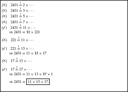
The only other small trick is the ability to find all of the prime numbers in order to divide by them. Figure 3-2 shows an example of brute-force factorization using such a list. Although for smaller numbers (only a few digits), the list of primes needed would be small, it would be prohibitive to have a list of all the prime numbers required for large factorization lying around. Furthermore, even checking to see if a large number is prime can be costly (since it would involve a very similar algorithm to that above).

The answer is that we would just hop through the list of all integers, skipping ones that are obviously not primes, like even numbers, those divisible by three, and so forth. For more details on implementations and behavior of this algorithm, see Reference [6].

We leave it as an exercise to the reader to implement the brute-force algorithm.

Analysis

In order to see how much time this takes to run, we need to know how many prime numbers there are. We could simply count them, which would be the only exact method. But there is a well-known rough approximation, saying that if we have a number a, then there are approximately

prime numbers less than or equal to a. In reality, there are a bit more than this, but this provides a good lower bound. In terms of the length of a (in binary digits), we have n = log₂a digits.

The running time will then be one division operation per prime number less than the square root of the number a, which has n/ 2 digits. Therefore, dividing by every prime number of less than

The storage requirements for this are simply storing the factors as we calculate them, and keeping track of where we are. This won't take up too much space; thus, we need not be worried at this point.

As terrible as this may seem when compared to other algorithms in terms of time complexity, it has the advantage that it always works. There is no randomness in its operation, and it has a fixed, known upper-bound. Few other algorithms discussed here have these properties. Also, other algorithms are not guaranteed to find complete prime factorizations (whereas this one does) and often rely on trial division to completely factor numbers less than some certain bound.

A method attributed to Fermat in 1643 [6] uses little more than normal integer arithmetic to siphon large factors from numbers. In fact, it doesn't even use division.^[35]

The algorithm works from a fact often learned in basic algebra:

(x + y) (x − y) = x² − y²

for any integers x and y. Fermat theorized using this to factor a number: If we can discover two squares such that our target number (a) is equal to the difference of the two squares (x² −y²), we then have two factors of the n, namely, (x + y) and(x − y).

Fermat's method just tries, essentially, to brute-force the answer by going through the possible squares and testing them. The algorithm is written out concisely in Reference [15], although I have changed some of the variable names for the following:

Fermat's Difference of Squares. Take an integer, a, to factor. The goal is to calculate x² and y² so that (x + y)(x −y) = x² −y² = a. In the following, d = x² − a (which should, eventually, be equal to y²).

For a simple example, Figure 3-3 shows this algorithm being run on the number 88.

Figure 3-3. Fermat's difference of squares method for finding factors of 88.

Analysis of Fermat's Difference of Squares

The running time of Fermat's difference of squares method is on the order of

Pollard has come up with several very clever mechanisms for factoring integers, as well as other ones we shall study below in this chapter.

Pollard's rho (ρ) method works by finding cycles in number patterns. For example, using the modular arithmetic from the previous chapter, we may want to successively square the number, say, 2, repeatedly modulo 14. This would result in a sequence

2, 4, 8, 2, 4, 8,...

This sequence repeats itself forever. Pollard figured out a way to have these sequences give us clues about the factors of numbers.

We'll show the algorithm, and then explain the nifty trick behind it.

Pollard's ρ. Factors an integer, a.

Why does this work? Well, the first leap of faith is that the function f (x) will randomly jaunt through the values in the field. Although it is fairly simple (just a square with a constant addition), it will work, in general.

The second notion here is what is going on with the function calls. The value B is "moving" through the values of the field (values modulo a) twice as "fast" (by calling the function f twice). This will give two pseudorandom sequences through the elements of the field.

Listing 3-3 shows a simple implementation of this program in Python, and Figure 3-4 shows an example run of the program.

The reason this algorithm is called the ρ algorithm is because, if drawn out on paper, the paths of the two values, A and B, chase each other around in a way that resembles the Greek letter ρ (see Figure 3-5).

Analysis of Pollard's ρ

The Pollard ρ algorithm has time complexity of approximately O (n¹/4) for finding a factor and no significant amount of storage [15]. Completely factoring a number will take slightly more time, but finding the first factor will usually take the longest.

Figure 3-4. Pollard's ρ factorization of 2,262,599, with b = 2, s = 2.

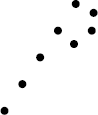
Figure 3-5. Figure showing the path of a run of the Pollard ρ algorithm. The path will eventually loop back upon itself, hence the name " ρ." The algorithm will detect this loop and use it to find a factor.

Example 3-3. Python code for Pollards ρ algorithm for factoring integers.

# Euclidean algorithm for GCD

def gcd(x, y):
 if y==0:
  return x
 else:
  return gcd(y, x % y)

# Stepping function

def f(x, n):
    return (x*x+3)%n

# Implements Pollard rho with simple starting conditions

def pollardrho(a):
    x = 2
    y = 2
    d = 1

    while d == 1:
        x = f(x, a)
        y = f(f(y, a), a)
        d = gcd(abs(x - y), a)

        if d>1 and a > d:
            return d
        if d == a:
            return −1

John M. Pollard also has another method attributed to him for factoring primes [12]. Pollard's p − 1 method requires that we have a list of primes up to some bound B. We can label the primes to be, say, p₁ = 2, followed by p₂ = 3, and p₃ = 5, and so on, all the way up to the bound B. There are already plenty of lists of primes to be found on the Internet, or they could be generated with a simple brute-force algorithm as described above, since we don't need very many of them (only a few thousand in many cases).

The algorithm works by Fermat's little theorem, that is, given a prime p and any integer b, then

We want to find p such that p is a prime factor of a, the number we are trying to factor. If L is some multiple of (p − 1), then p | gcd(b^L − 1, a). The best way to try to get L to be a multiple of (p − 1) is to have L be a multiple of several prime factors. We can't compute b^L mod p, but we can compute b^L mod a. The algorithm works by computing

Pollard's p − 1 . Factors an integer, a, given a set of primes, p1, . . ., pk.

I won't show an implementation of this algorithm, since it requires such a large list of primes.

A method of factoring based on square forms, to be discussed in this section, was devised by Shanks in References [9] and [14].

Before we dive in to the Square Forms Factorization method (SQUFOF), I'll first set up a little of the mathematics.

Let the ordered triple of integers (a, b, c) correspond to all values of

ax² + bxy + cy²

for all integers x and y. We say that (a, b, c) represents some value m if, and only if, we can find two values x and y such that ax² + bxy + cy² = m.

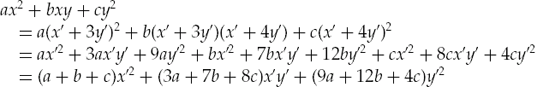
We say that two forms of (a, b, c) are equivalent if the two forms represent the same set of numbers. One way in which this can be done is by a linear change of variables of x and y, where x' = Ax + By, y' = Cx + Dy, and AD − BC = 1 or −1. For example, if A = 1, B = 3, C = 1, and D = 4, then we would have x' = x + 3y, y' = x + 4y, and

For example, (1, 1, 2) and (4, 26, 29) are equivalent.

This has two implications: The two forms represent the same set of numbers, and their discriminants of the form

D = b² − 4ac

will be the same.

A square form is a form of (a, b, c), where a = r² for some integer r — that is, a is a perfect square.

We will want to find a reduced square form, similar to finding the smallest CSR earlier. This is not hard ifD < 0, but if D> 0, then we define a form as reduced if

The SQUFOF algorithm works by finding equivalent reduced forms related to the integer we want to factor.

For more information on implementing the square form factorization, see, for example, Stephen McMath's SQUFOF analysis paper [9].

The elliptic curve factorization method (ECM) works similarly to Pollard's p − 1 algorithm, only instead of using the field of integers modulo p, weusean elliptic curve group based on a randomly chosen elliptic curve. Since many of the same principles work with elliptic curve groups, the idea behind Pollard's p − 1 also works here. The advantage is that the operations tend to take less time. (It's easier to multiply and add smaller numbers required for elliptic curves than the larger numbers for exponential-based group multiplication.) ECM was originally developed by Lenstra Jr. [7].

As before, we assume that we have a list of all of the primes {2, 3, 5,... } stored as {p₁,p₂,p₃,...} less than some bound B.

Elliptic Curve Factorization Method. The elliptic curve will be generated and used to try to find a factor of the integer a. The elliptic curve operations and coordinates will be taken modulo a.

Furthermore, g is not guaranteed to be prime, but merely a factor.

Analysis of ECM

If p is the least prime dividing the integer a to be factored, then the expected time to find the factor is approximately

The first term in this will typically dominate, giving a number a bit less than e^p.

In the worst-case scenario, when a is the product of two large and similar magnitude primes, then the running time is approximately

This is going to be a bit less than eⁿ, but not so much. In both cases, the average and worst case, these are still exponential running times.

The continued fraction factorization method is introduced in Reference [10]. The following explanation draws on this paper, as well as the material in References [9] and [15].

First, let's learn some new notation. If we wish to convey "x rounded down to the nearest integer," we can succinctly denote this using the floor function [x]. This means that [5.5] = 5, [−1.1] = −2 and [3] = 3, for example. I have avoided using this notation before, but it will be necessary in the following sections.

One more quick definition. A continued fraction is a fraction that has an infinite representation. For example:

Furthermore, a continued fraction for any number (say, c) can be constructed noting that c = [c] + c − [c], or

Furthermore, with a continued fraction form like the above (written compactly as [c₀, c₁, ..., c_k]), we can find A_k//B_k, the rational number it represents, by the following method:

The above algorithm will eventually terminate if the number being represented is irrational. Otherwise, it continues forever.

Using this method, we can now compute quadratic residues, Q_i — remainders when subtracting a squared number. The quadratic residues we are interested in are from

We will use the quadratic residues to derive a continued fraction sequence for

We need an upper-bound on factors we will consider, B. The algorithm for exploiting this works by factoring each Q_i as we calculate it, and if it is B-smooth (contains no prime factors less than B), we record it with the corresponding A_i. After we have collected a large number of these pairs, we look at the exponents of the factors of each Q_i (modulo 2) and find equivalences between them. These will represent a system of equations of the form:

x² ≡ y² (mod n)

When x is not equal to y, we use the same principle of Fermat's difference of squares to factor n.

The reason this works is that a square is going to have even numbers as exponents of prime factors. If we have two numbers that when multiplied together (adding their exponents) have even numbers in the exponent, we have a perfect square.

Analysis of CFRAC

Although the above work is fairly complex and involved, the above method saves an extraordinary amount of time. Using the CFRAC method to factor an integer will yield a running time on the order of

For reference, a normal exponential algorithm might be about

Two final methods that we shall not delve too deeply into are the quadratic sieve (QS) and the general number field sieve (GNFS). Both rely on the principle of Fermat's difference of squares and produce factors using this idea.

For QS, the idea is very similar to the continued fraction method in the previous section, using sieve instead of trial division for factorizations. The running time of QS tends to be on the order of about

A lot of focus has been on the GNFS, since it is the fastest known method for factoring large integers, or in testing the primality of extremely large integers.

The GNFS works in three basic parts. First, the algorithm finds an irreducible polynomial that has a zero modulo n [where n is the modulo base we are working with, so that gcd(x − y, n)> 1, to find a factor]. Next, we find squares of a certain form that will likely yield factors. Then we find the square roots.

The "sieve" in the GNFS comes from the finding of squares in the second step. The special form that the squares come into involves calculating products of the sums of relatively prime integers. These relatively prime integers are calculated using sieving techniques.

For more information on the GNFS, see, for example, References [2] and [8].

There are, in general, two brute-force methods for computing a discrete logarithm.

If the number of elements in the field is small enough (less than a few billion or so, at least with today's computers), we can pre-compute and store all possible values of the generator raised to an exponent. This will give us a lookup table, so that any particular problem will take only as much time as it takes to look up the answer.

Obviously, there are some strong limitations here. With large fields, we can have extremely large tables. At some point, we aren't going to have enough storage space to store these tables.

At the other end of the spectrum is the second method for computing a discrete logarithm. Here, each time we want to solve a discrete logarithm problem, we try each and every exponent of our generator. This method takes the most amount of time during actual computation but has the advantage of no pre-computation.

It's easy to see that there should be a trade-off somewhere, between pre-computing everything or doing all the work every time. However, we need to be a little clever in choosing that trade-off point. Some people have put a lot of cleverness into these trade-off points, discussed below (and similar concepts are discussed in later chapters).

The baby-step giant-step algorithm is one of the simplest trade-offs on time versus space, in that we are using some pre-computed values to help us compute the answers we need below.

Baby-Step Giant-Step. For the following algorithm, assume we are working in finite field over Z_p, solving a^x = b in Z_p for x.

Basically, we are computing b × h^j in the loop and terminating when it equals some aⁱ, where 0 ≤ i < L, giving us

b × h^j = aⁱ

b × ((a⁻¹)^L)^j = aⁱ

b × a^{− Lj} = aⁱ

b = aⁱ. a ^Lj

b = a^Lj+i

Therefore, the discrete logarithm of b is Lj + i.

Baby-Step Giant-Step Analysis

The baby-step giant-step algorithm represents a hybrid of the first two brute-force methods. It has on the order of

Like the previous brute-force methods, this method will find us an answer eventually, and there is no randomness involved. However, the space requirements are fairly large. For example, when p has hundreds or thousands of digits, then

Pollard's ρ method for discrete logarithms [11] relies on a similar principle as Pollard's ρ method for factoring — that is, we are looking for a cycle when stepping through exponents of random elements.

Here, assume that the group we are working with (the field) is the set of integers between 0 and p − 1 (written as Z_p) along with normal addition and multiplication.

To perform Pollard's ρ algorithm for discrete logarithms, we partition the set of all integers between 0 and p − 1 into three partitions of roughly equal size: P₀, P₁, and P₂. These three sets can be simple, such as either the integers below p divided into three contiguous sets (the first third of numbers less than p, the second third, the third third), or split by the remainder of the number when divided by 3 (so that 2 belongs in P₂, 10 belongs in P₁, and 15 belongs in P₀).

The algorithm expects to solve the problem a^x = b in the group G, thus it takes a and b as arguments.

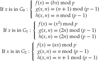
It relies on three functions to operate: the function f, which takes one argument — an integer modulo p — and returns an integer modulo p; the function g, which takes an integer modulo p and a normal integer and returns an integer modulo p − 1; and a function h that takes an integer modulo p and an integer and returns an integer module p − 1.

The functions are defined based on the partition they are in. Thus:

Pollard's ρ for Discrete Logarithms.

Analysis of Pollard's ρ for Discrete Logarithms

Pollard's ρ solves the discrete logarithm with running time on the order of

This makes it a great candidate for small discrete logarithm problems, where

Pollard also proposed a generalization of the ρ algorithm for discrete logarithms, called the λ method (λ is the Greek letter lambda). Pollard's λ method of finding a discrete logarithm is a neat algorithm — interesting name, an amusing description, and very clever. Here, we want to compute the discrete logarithm for g^x = h in a group G where we have some bound on x, such that a ≤ x < b.

The following description is derived from References [11] and [15]. This method is sometimes called the method of two kangaroos (or hares, or rabbits, depending on the author). The concept is that two kangaroos (representing iterative functions) are going to go for some "hops" around the number field defined by the integer we wish to factor. These two kangaroos (or 'roos, as we like to say) consist of a tame one, controlled by us and represented by T, and a wild one that we are trying to catch, W.

The tame 'roo, T, starts at a random point,t₀ = g^b, while W starts at w₀ = h = g^x. Define d₀(T) = b, the initial "distance" from the "origin" that the tame 'roo is hopping, and let d₀(W) = 0, the initial distance of our wild 'roo from h.

Let S = {g^s1, ..., g^sk} be a set of jumps, and let G be partitioned into k pieces G₁, G₂, ..., G_k, with 1 ≤ f (g) ≤ k being a function telling to which partition g belongs. These exponents of g in S should be positive and small compared to (b −a). Most often, we will pick these numbers to be powers of 2 (2ⁱ). These are the hops of both kangaroos.

Now, the two kangaroos are going to hop.T goes from t_i to

The tame 'roo will have distance

Similarly, W goes from w _i to

giving the wild 'roo distance

d_i+1 (W) = d_i (W) + s_f (_wi)

Eventually, T will come to rest at some position t_m, setting a trap to catch W. If ever d_n (W) > d_m (T), then the wild kangaroo has hopped too far, and we reset W to start at w₀ = hg^z, for some small integer z > 0.

Analysis of Pollard's λ

To make this work, we need to set the s_i values so that they are about 0.5

The index calculus method provides a method analagous to quadratic and number field sieves of factoring, shown above. This method is particularly well suited to solving the discrete logarithm on multiplicative groups modulo prime numbers. It was first described as the first subexponential discrete logarithm function by Adleman and Demarrais [1].

In general, this can be a very fast method over multiplicative groups, with on the order of e

For more information on the index calculus method, please refer to Reference [1].