
So far, we have covered basic mathematics for studying encryption algorithms and even learned how to use several forms of asymmetric algorithms (ones that usually have a split key, a private and a public key). Before progressing further into modern symmetric algorithms (ones where both parties share the same key), we need to have an overview of the different forms of block ciphers.
To review, a block cipher is one that takes more than one character (or bit) at a time, processes them together (either encryption or decryption), and outputs another block. A block usually consists of a contiguous set of bits that is a power of 2 in size; common sizes are 32, 64, 128, and 256 bits. (A block size of 8 or 16 bits would possibly mean that it is not so much a stream cipher, but more just a character-for-character cipher, like we studied earlier.)
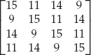
The simplest example of a block cipher is the columnar transposition cipher studied above. However, columnar transposition ciphers are based on character transformations and have variable block size, depending on the column size chosen. The ciphers studied from here on out are used in digital computers and thus will normally have bit operations.
Before the 20th century, people normally wanted to send messages consisting of text. This required operations on letters and blocks of letters, since these messages were written, either by hand or perhaps type; thus, the tools and techniques of cryptography were focused on letters and blocks of letters. In the modern age, we are concerned with digital information, such as text files, audio, video, and software, typically transmitted on computers or computer-like devices (e.g., phones, ATMs). The standard way to represent these forms of data is in bits, bytes, and words.
The following section presents a quick review of the basic building blocks of modern cryptography, such as bits and bytes. The rest of the chapter is devoted to more complicated structures of modern ciphers that we need to understand, so that we can break them in further chapters. I also present the inner workings of a few of the most popular targets for modern cryptanalysis (because of their widespread use), such as DES and AES.
This chapter is not an exhaustive study of modern cryptography. There are many good books on cryptography: the building of ciphers, as well as tools and techniques for doing so [11, 16]. Here, we wish to understand the basic structure of most ciphers, especially related to how we can manipulate those structures in later chapters.
A bit, as seen above but not quite defined, is a binary digit that is either a 0 or a 1. The standard byte is composed of 8 contiguous bits, representing values 0 through 255 (assuming we are only concerned with non-negative integers). When writing a byte in terms of its 8 bits, we write them as we do with normal numbers in decimal notation, in most significant bit order — as in, left-to-right, the more important, and hence "bigger," bits written first. For example, the byte representing the number 130 written in binary is
10000010
There is such a thing as least significant bit order, where the bits are essentially written backwards in a byte (certain communication protocols use this, for example), but I shall not discuss this further.
The next major organization of bits is the word, the size of which is dependent on the native size of the CPU's arithmetic register. Normally, this is 32 bits, although 64-bit words have been becoming common for quite some time; less commonly seen are 16-bit and 128-bit words.
We again have two ways of writing down words as combinations of bytes. The most significant byte (MSB) writes the "biggest" and most important bytes first, which would be analogous to the most significant bit order first. This is also called big endian, since the "big end" is first. For a 32-bit word, values between 0 and 4,294,967,295 (= 232 – 1) can be represented (again, assuming we are representing non-negative integers). In big-endian binary, we would write the decimal number 1,048,580 (= 220 + 22 = 1,048,576 + 4) as
00000000 00010000 00000000 00000100
Equivalently, we can write it in big-endian hexadecimal (base 16) by using a conversion table between binary and hexadecimal (see Table 4-1).
The above number, 1,048,580, written in big-endian hexadecimal ("hex") would be 00 10 00 04.
There is also another way to represent words in bytes: least significant byte (LSB) or little endian (for "little end" first). Basically, just take the previous way of writing it, and reverse it. The most confusing part is that the bits are still written in most significant bit order.
Table 4-1. Binary to Hexadecimal Conversion Table
BINARY | HEX | BINARY | HEX |
|---|---|---|---|
0000 | 0 | 1000 | 8 |
0001 | 1 | 1001 | 9 |
0010 | 2 | 1010 | A |
0011 | 3 | 1011 | B |
0100 | 4 | 1100 | C |
0101 | 5 | 1101 | D |
0110 | 6 | 1110 | E |
0111 | 7 | 1111 | F |
This would make the above number, 1,048,580, written in little-endian hexadecimal as 04 00 10 00 and in binary as
00000100 00000000 00010000 00000000
There is no consensus in the computer architecture community on which one of these methods of writing words is "better": They both have their advantages and disadvantages.
I will always be very clear which method is being used in which particular cipher, as different ciphers have adopted different conventions.
There are a few basic operations that are useful to understand. Before, we studied basic operations on normal text characters, such as by shifting the characters using alphabets. Now, we are concerned with operations on binary data.
The AND operator (sometimes written as &, ·, or ×) operates on 2 bits. The result is a 1 if both operands are 1, and 0 otherwise (and hence, only 1 if the first operand "and" the second operand are 1). The reason symbols for multiplication are used for AND is that this operates identically to numerically multiplying the binary operands.
The OR operator (sometimes written as | or +) also takes two operands, and produces a 1 if either the first operand "or" the second operand is a 1 (or both), and 0 only if both are 0. Sometimes this can be represented with the plus symbol, since it operates similarly to addition, except that in this case, 1 + 1 = 1 (or 1| 1 = 1), since we only have 1 bit to represent the output.
The XOR (exclusive-OR, also called EOR) operator, commonly written as ^ (especially in code) and ⊉ (often in text), operates the same as the OR operator, except that it is 0 if both arguments are 1. Hence, it is 1 if either argument is 1, but not both, and 0 if neither is 1.
XOR has many uses. For example, it can be used to flip bits. Given a bit A (either 0 or 1), calculating A ⊉ 1 will give the result of flipping A (producing a result that is opposite of A).
Table 4-2 shows the outputs of the AND, OR, and XOR bitwise operators.
The final basic operation is the bitwise NOT operator. This operator takes only a single operand and simply reverses it, so that a 0 becomes a 1 and a 1 becomes a 0. This is typically represented, for a value a, as ~ a, a, or ¬ a (in this book, we mostly use the latter). This can be combined with the above binary operators, by taking the inverse of the normal output. The most used of these operators are NAND and NOR.
All of these operators naturally extend to the byte and word level by simply using the bitwise operation on each corresponding pair of bits in the two bytes or words. For example, let a = A7 and b = 42 (both in hexadecimal). Then a &b = 02, a |b = E7, and a ⊉ b = E5.
In this book, I will try to show bits numbered from 0 up, with bit 0 being the least significant. When possible, I will try to stick with MSB (big endian) byte order, and most significant bit order as well. One final notation that is handy when specifying cryptographic algorithms is a notation of how to glue together various bits. This glue (or concatenation) is usually denoted with the || symbol. For example, the simple byte, written in binary as 01101101 would be written as
0 || 1 || 1 || 0 || 1 || 1 || 0 || 1
We might also specify some temporary value as x and want to specify the individual bits, such as x0, x1, and so on. If x is a 4-bit value, we can use the above notation to write
x = x3 || x2 || x1 || x0
Because we may be working with large structures with dozens or hundreds of bits, it can sometimes be useful to use the same glue operator to signify
concatenating larger structures, too. For example, if y is a 64-bit value and we want to reference 8 of its byte values, we might write them as
y = y7 || y6 || y5 || y4 || y3 || y2 || y1 || y0
In this case, we will let y0 be the least significant 8 bits, y1 the next bits, and so forth.
I will try to be clear when specifying the sizes of variables, so that there will be as little confusion as possible. Even I have had some interesting problems when implementing ciphers, only to discover it is because the sizes were not properly specified, so the various pieces did not fit together.
Again, I find it useful to have some code snippets in this chapter so that you can more easily see these algorithms in action.
And again, as in the previous chapter, I will have the examples in Python. This is for several reasons:
Python has good support for array operations.
Python code tends to be short.
Python code tends to be easy to read.
I already introduced Python, and it would be silly to introduce another language.
I won't have time to introduce every concept used, but I will try not to let something particularly confusing slip through. It is my intention that the examples will provide illumination and not further confusion.
With that little bit of introductory material out of the way, we can start exploring how we build block ciphers using some of the tools that we have developed, as well as a few more additional tools we shall build in the following sections.
One concept has reigned up to this point: We take some chunk of plaintext, subject it to a single process, and after that single process is completed, we have that ciphertext. This is not the case with most real-world ciphers today.
Modern ciphers are designed with the realization that having a single, large, complex operation can be impractical. Moreover, relying on only a single technique, such as a columnar transposition, is putting all of our eggs in one basket, so to speak: All of security is dependent on a single principle.
One of the key concepts in modern cryptography is the product cipher — a type of cipher that consists of several operations conducted in sequences and loops, churning the output again and again. The operations used are often those seen so far: substitutions, permutations, arithmetic, and so on. Ideally, the resilience of the resulting ciphertext will be significantly more than the individual strengths of the underlying techniques.
A simple example from Chapter 1 illustrates this concept. Instead of just performing a polyalphabetic cipher (susceptible to Kasiski's method) or a columnar transposition cipher (subject to the sliding window technique with digraph and trigraph analysis), we can combine both techniques — first perform a keyed substitution, letter-by-letter, on the original plaintext, and then run the output of that through the columnar transposition matrix. In this case, the resulting ciphertext would be completely immune to both Kasiski's method and to windowed digraph and trigraph analysis, defeating all of the techniques previously developed.
However, using a small sequence of polyalphabetic and columnar transposition ciphers in sequence does not make a cipher robust enough for modern use. Anyone who can guess which combination of techniques is being used can easily combine several types of analysis at once. There are a fairly limited number of combinations of these simple techniques to be used. And even so, these combinations could be easily broken by modern computing speeds. And finally, because most modern data that need to be encrypted are binary data from computers, and not handwritten or typed messages, these techniques are ill-suited for most current needs.
In Chapter 1 I discussed two useful tools: substitutions (as in mono- and polyalphabetic substitution ciphers) and transpositions (as in columnar transposition ciphers). It turns out that digital counterparts to these exist and are widely used in modern cryptography.
The terminology for a digital substitution is called a substitution box, or S-box. The term box comes from the fact that it is regarded as a simple function: It merely accepts some small input and gives the resulting output, using some simple function or lookup table. When shown graphically, S-boxes are drawn as simple boxes, as in Figure 4-1.

S-boxes normally are associated with a size, referring to their input and output sizes (which are usually the same, although they can be different). For example, here is a representation of a 3-bit S-box, called simply S :
S[0] = 7 S[3] = 4 S[6] = 0
S[1] = 6 S[4] = 3 S[7] = 1
S[2] = 5 S[5] = 2
This demonstrates one of the simpler methods of showing an S-box: merely listing the output for every input. As we can see, this S-box, S, almost reverses the numbers (so that 0 outputs 7, 1 outputs 6, etc.), except the last two entries for S [6] and S [7].
We can also specify this S-box by merely writing the outputs only: We assume that the inputs are implicitly numbered between 0 and 7 (since 7 = 23 − 1). In general, they will be numbered between 0 and 2b − 1, where b is the input bit size. Using this implicit notation, we have S written as
[7, 6, 5, 4, 3, 2, 0, 1]
Of course, in the above S-box, I never specified which representation of bits this represents: most significant or least significant. A word of caution: Some ciphers do actually use least significant bit order (such as DES), even though this is fairly uncommon in most other digital computing. This can be very confusing if you are used to looking at ciphers in most significant bit order, and vice versa.
As specified above, S-boxes may have different sizes for inputs and outputs. For example, an S-box may take a 6-bit input, but only produce a 4-bit output. In this case, many of the outputs will be repeated. For the exact opposite case, with, say, a 4-bit input and 6-bit output, there will be several outputs that are not generated.
Sometimes S-boxes are derived from simpler moves. For example, we could have a 4-bit S-box that merely performs, for a 4-bit input x, the operation 4 −x mod 16, and gives the result. The S-box spelled out would be
[4, 3, 2, 1, 0, 15, 14, 13, 12, 11, 10, 9, 8, 7, 6, 5]
S-boxes have some advantages, as we can see. They can be very random, with little correspondence between any input bits and output bits, and have few discernible patterns.
One primary disadvantage is size: They simply take a lot of space to describe. The 8-bit S-box for Rijndael, shown in Figure 4-2, takes a lot of space and requires implementing code to store the table in memory (although it can also be represented as a mathematical function, but this would require more computation at run time).
Another tool, the permutation box (or simply, P-box), is similar to an S-box but has a slightly different trade-off: A P-box is usually smaller in size and operates on more bits.
A P-box provides similar functionality to transpositions in classical cryptography. The purpose of the permutation box is to permute the bits: shuffle them around but without changing them.
P-boxes operate by mapping each input value to a different output value by a lookup table — each bit is moved to a fixed position in the output. Most P-boxes simply permute the bits: one input to one output. However, in some ciphers (such as DES), there are expansive and selective permutations as well, where the number of output bits is greater (some bits are copied) or smaller (some bits are discarded), respectively.
P-boxes are normally specified in a similar notation to S-boxes, only instead of representing outputs for a particular input, they specify where a particular bit is mapped to. Assume that we number the bits from 0 to 2b − 1, where b is the size of the P-box input, in bits. The output bits will also be numbered from 0 to 2c − 1, where c is the size of the P-box output, in bits.

For example, an 8-bit P-box might be specified as
P = [351047 62]
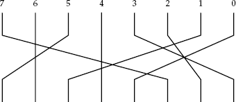
This stands for P[0] = 3, P[1] = 5, P[2] = 1, ..., P[6] = 6, P[7] = 2. The operation means to take bit 0 of the input and copy it to bit 3 of the output. Also take bit 1 of the input, and copy it to bit 5 of the output, and so forth. (Note that not all bits necessarily map to other bits — e.g., in this P-box, bits 4 and 6 map to themselves.) The example in Figure 4-3 illustrates this concept graphically.
For the preceding P-box, assume that the bits are numbered in increasing order of significance (0 being the least significant bit, 7 the most). Then, for example, the input of 00 will correspond to 00. In hexadecimal (using big-endian notation), the input 01 would correspond to 20, and 33 would correspond to B8.
A few things to note about P-boxes: They aren't as random as S-boxes — there is a one-to-one correspondence of bits from the input to the output. P-boxes also take a lot less space to specify than S-boxes: The 8-bit P-box could be written out in very little space. A 16-bit P-box could be written as a list of 16 numbers, but it would require a list of 65,536 numbers to fully specify a 16-bit S-box.
However, technically speaking, P-boxes are S-boxes, just with a more compact form. This is because they are simply a mapping of input values to output values and can be represented as a simple lookup table, such as an S-box. The P-box representation is merely a shortcut, albeit a very handy one.
If we look at any of the previously mentioned structures, though, we can see that they should not be used alone. A trivial cipher can be obtained by just using an S-box on an input, or a P-box, or even XORing each input byte with a fixed number. None of these techniques provides adequate security, though: The first two allow anyone with knowledge of the S-box or P-box to immediately decrypt a message, and with a simple XOR, anyone who knows the particular value of one byte in both plaintext and ciphertext could immediately derive the key.
For these reasons, I will use the above concept of a product cipher to combine each of these concepts — bitwise operations, S-boxes, and P-boxes — to create a very complicated structure. We won't limit ourselves to just these particular operations and boxes, but the ones explained so far represent the core of what is used in most modern cryptographic algorithms.

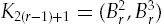
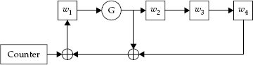
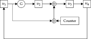
Another tool used in the construction of ciphers is a shift register. Look at Figure 4-4, one of two shift registers in Skipjack (called Rule A and Rule B), for an example of how a shift register operates.
Typically, a shift register works by taking the input and splitting it into several portions; thus, in this case, w = w1 || w2 || w3 || w4 || is our input. Then, the circuit is iterated several times. In this diagram, G represents a permutation operation. Thus, after one round through the algorithm, w2 will get the permutation of w1;w3 will be the XOR of the old w2, the counter, and the old w1; and w4 will get the old value of w3; while w1 gets the old value of w4. This iteration is repeated many times (in Skipjack, it iterates eight times in two different locations).
Shift registers are meant to mimic the way many circuits and machines were designed to work, by churning the data in steps. These are also designed with parallelism in mind: While one piece of circuitry is performing one part of the computation, another can be computing with a different part of the data, to be used in following steps.
The first natural extension of the above simple techniques is to merely start combining them. A substitution–permutation network (SPN) is just that: It chains the output of one or more S-boxes with one or more P-boxes, or vice versa. The concept is similar to chaining together simple substitution ciphers of text and transposition ciphers: We have one layer substituting values for other values, thereby adding a lot of confusion (in that it is a bit harder to see where the output comes from). We then have another layer mixing the output bits from one or more S-boxes and jumbling them together, contributing primarily to diffusion (in that input bits influence a lot of output bits).
However, up until this point, we are still going to have trouble with the output being trivially related to the input: Simply knowing the combinations of S-boxes and P-boxes can let us derive one from the other. We need a way of adding a key into the system so that only parties privy to the key will be able to encrypt and decrypt messages.
The most common mechanism for adding keys to the above system is to compute some function of the key to give a set of bits, referred to as the key schedule. These bits from the key schedule are then usually integrated into the cipher somehow, normally by XORing them together with intermediate bits in the cipher (such as the input of some S-boxes).
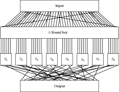
The most common way of forming an SPN is to have many (usually different) S-boxes and P-boxes, with their inputs and outputs chained together. For example, see Figure 4-5. When we chain them together like this, we may XOR in the key schedule bits several times. We call these key schedule bits and not just the key bits because, as I said above, these bits are merely derived from the key. Some may be identical to the key, but, for example, we may use different subsets of the key bits at different parts of the network (maybe shifted, or inverted at different parts).

As Reference [4] points out, SPN ciphers are ideal for demonstrating several cryptanalytic techniques.
There is a need for a cipher that is easy enough for you to easily implement and see results of various techniques, while still being complicated enough to be useful. For that, we shall create a cipher call EASY1 in this section. We'll use it in later chapters to demonstrate some of the methods of cryptanalysis.
EASY1 is a 36-bit block cipher, with an 18-bit key. EASY1 works by splitting its input into 6-bit segments, running them through S-boxes, concatenating the results back together, permuting them, and then XORing the results with the key. The key is just copied side-by-side to become a 36-bit key (both the "left half" and "right half" of the cipher bits are XORed with the same key).
We will use various numbers of rounds at different times, usually low numbers.
The 6-bit S-boxes in EASY1 are all the same:
[16, 42, 28, 3, 26, 0, 31, 46, 27, 14, 49, 62, 37, 56, 23, 6, 40, 48, 53, 8,
20, 25, 33, 1, 2, 63, 15, 34, 55, 21, 39, 57, 54, 45, 47, 13, 7, 44, 61, 9,
60, 32, 22, 29, 52, 19, 12, 50, 5, 51, 11, 18, 59, 41, 36, 30, 17, 38, 10, 4,
                               58, 43, 35, 24]
This is represented in the more compact, array form: The first element is the substitution for 0, the second for 1, and so forth. Hence, an input of 0 is replaced by 16, 1 by 42, and so on. The P-box is a large, 36-bit P-box, represented by
[24, 5, 15, 23, 14, 32, 19, 18, 26, 17, 6, 12, 34, 9, 8, 20, 28, 0, 2, 21, 29,
           11, 33, 22, 30, 31, 1, 25, 3, 35, 16, 13, 27, 7, 10, 4]
Our goal with EASY1 is that it should be easy to understand and fast to derive keys without the use of cryptanalysis (so answers can be verified).
I'll provide some quick code to perform EASY1.
Here, I show a simple EASY1 implementation in Python. For simplicity, I will make the implementation generic so that different values can be easily put in and tested.
Assume that the S-box is input as a simple array in a variable called s, and that the P-box is also stored as an array in s.
We can make generic S-box and P-box functions. The S-box function is simple: Use the argument as an index into the array, which will return the appropriate value. The P-box implementation is a bit trickier, as shown in Listing 4-1.
Example 4-1. Python code for the EASY1 S-box and P-box.
########################################### S-box function##########################################defsbox(x):returns[x]########################################### P-box function##########################################defpbox(x):# if the texts are more than 32 bits,# then we have to use longsy = 0l# For each bit to be shuffledforiinrange(len(p)):# If the original bit position# is a 1, then make the result# bit position have a 1if(x & (1l << i)) != 0: y = y^(1l << p[i])returny
In Listing 4-1, we first have to introduce some cumbersome notation: The "l" (or "L") modifier specifies that the number may grow to become more than 32 bits (which is the size of a normal Python integer). Although it can automatically grow, it gives a lot of warnings if we don't tell Python we are expecting this, by specifying that we want a long integer, meaning that it can be much bigger. (The values of the bits of the output that are not copied are all zeros.)
The rest of the code to implement the P-box is not too bad. We have to do an ugly calculation that, for each bit position in the P-box, determines if that input bit is set. If so, then it determines which bit the set bit maps to in the output and sets it as well. All bits not set in this way are set to zero.
The next piece of code (Listing 4-2) is used for splitting apart the pieces to be fed to the S-boxes and then put back together — hence the mux (multiplex, or combine) and demux (demultiplex, or break apart) functions.
Example 4-2. Python code for the EASY1 multiplexing and demultiplexing.
########################################### Takes 36-bit to six 6-bit values# and vice-versa##########################################defdemux(x): y =[]foriinrange(0,6): y.append((x >> (i * 6)) & 0x3f)returnydefmux(x): y = 0lforiinrange(0,6): y = y ^ (x[i] << (i * 6))returny
The trickiest part of this code is the use of the bit shift operators, which simply take the left-hand side of the expression and shift the bits left (for <<) or right (for >>) by the number on the right. The demux function also uses an AND operation by 0x3F, which is the bit mask representing the binary expression 111111 — that is, six 1's, which will drop all the bits to the left, returning only the rightmost six bits.
Finally, we write one last helper function: the code to XOR in the keys. This code is shown in Listing 4-3 — nothing too fancy there.
Example 4-3. Python code for EASY1 key XORing.
########################################### Key mixing##########################################defmix(p, k): v = [] key = demux(k)foriinrange(0,6): v.append(p[i] ^ key[i])returnv
After all of these helper functions, we can put in the code to do the actual encryption: the round function and a wrapper function (encrypt). This code is shown in Listing 4-4.
Example 4-4. Python code for EASY1 encryption.
########################################### Round function##########################################defround(p,k): u = []# Calculate the S-boxesforxindemux(p): u.append(sbox(x))# Run through the P-boxv = demux(pbox(mux(u)))# XOR in the keyw = mix(v,k)# Glue back together, returnreturnmux(w)########################################### Encryption##########################################defencrypt(p, rounds): x = pforiinrange(rounds): x = round(x, key)returnx
To complete this code roundup, we have the decryption code (shown in Listing 4-5).
Example 4-5. Python code for EASY1 decryption
########################################### Opposite of the round function##########################################defunround(c, k): x = demux(c)
u = mix(x, k) v = demux(apbox(mux(u))) w = []forsinv: w.append(asbox(s))returnmux(w)########################################### Decryption function##########################################defdecrypt(c, k): x = cforiinrange(rounds): x = deround(x, key)returnx
SPNs can be used alone (as a complete cipher, such as AES), or, for example, as part of a Feistel structure (see the next section).
One disadvantage to many types of ciphers, including substitution–permutation networks, is that two separate operations are required: encryption and decryption. Most algorithms require separate software routines or hardware to implement the two operations. When writing a cryptographic suite for an ASIC (a fixed, silicon chip), there is often a premium on space available: Implementing two separate functions, one for encryption and one for decryption, will naturally take up about twice as much space.
Luckily, there is a technique that allows both encryption and decryption to be performed with nearly identical pieces of code, which has obvious cost-saving benefits.
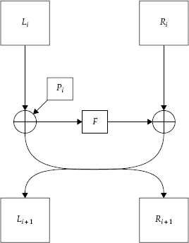
This now-common structure for modern ciphers was invented by Horst Feistel and is naturally called the Feistel structure. The basic technique is simple: Instead of developing two different algorithms (one for encryption, one for decryption), we develop one simple round function that churns half a block of data at a time. The round function is often denoted f and usually takes two inputs: a half-sized block and a round key. We then cleverly arrange the inputs and outputs to create encryption and decryption mechanisms for the whole block in the following manners.
For a particular structure, slight variations of the same Feistel structure are common between encryption and decryption rounds — different at least in key choice (this is called the key schedule), and sometimes in other parameters, or even the the workings of the structure itself.
Feistel ciphers typically work by taking half of the input at any round and XORing it with the output of the Feistel structure. This is then, in the next round, XORed with the other half, and the two halves are swapped, and the Feistel structure is computed and XORed in again. The two "halves" are not necessarily of equal length (which are called unbalanced).
Basic Feistel Encryption Algorithm. The basic Feistel encryption algorithm structure is r rounds long, with the round function f.
Split the initial plaintext, P, into two halves: The "left half" (L0) consists of the most significant bits, and the "right half" (R0) consists of the least significant bits.
For each round, i = 1, ..., r, do the following:
Calculate Ri = Li−1 ⊉ f (Ri−1, Ki), that is, the previous left half XORed with the round function (whose arguments are the previous right half and the current round key).
Calculate Li = Ri−1.
This structure will make more sense after looking at Figure 4-6, which shows the encryption in action.
The algorithm then terminates after the appropriate number of rounds, with the output ciphertext, C, obtained by concatenating the two halves after r rounds: Lr and Rr. For example, with three rounds, we would have the following progression:
R0
L0
R1 = L0 ⊉ f (R0, K1)
L1 = R0
R2 = L1 ⊉ f (R1, K2)
L2 = R1
R3 = L2 ⊉ f (R2, K3)
L3 = R2
Now, the nifty part of the Feistel structure we can see here at the end: If we have the ciphertext, L3 and R3, then that means we also have R2 (since L3 = R2). The party doing the decrypting will also know the key and thus will then know the appropriate value of the key schedule, K3, allowing the party to calculate f (R2, K3). Now note that
R3 = L2 + f (R2, K3)
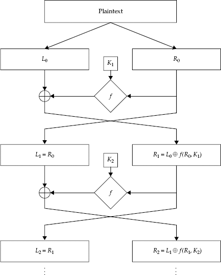
Figure 4-6. The Feistel structure for the first two rounds. The remaining rounds just repeat the structure.
from the above encryption. We can then rewrite this (by exchanging L2 and R3 due to the symmetry of XOR) to obtain
L2 = R3 ⊉ f (R2, K3)
We thus obtain the previous round's intermediate ciphertext, L2 and R2. Repeating this again and again will eventually reveal the original plaintext, as shown in the following example:
L3
R3
R2 = L3
L2 = R3 ⊉ f (R2, K3)
R1 = L2
L1 = R2 ⊉ f (R1, K2)
R0 = L1
L0 = R1 ⊉ f (R0, K1)
We can now generalize the decryption operation to work with any number of rounds.
Basic Feistel Decryption Algorithm. Computes a basic Feistel operation of r rounds, with a round function f, and key schedule (K1, K2, ..., Kr).
Split the ciphertext, C, into two halves: The "left half" (Lr) consists of the most significant bits, and the "right half" (Rr) consists of the least significant bits.
For each round, i = r − 1, ..., 0, do the following:
Set Ri = Li+1.
Set Li = Ri+1 ⊉ f (Ri, Ki+1).
As we can see, for decryption, the operations are nearly identical to the encryption algorithm. The primary difference is that the keys (Ki) are submitted in reverse order.
Ciphers that use the above Feistel structure have several notable properties.
The round function can be relatively simple, as the structure is normally iterated numerous times. Typically 4, 8, 16, and 32 rounds are common.
Encryption and decryption, for the most part, can use identical structures: The round function does most of the work for both operations. (Encryption and decryption can still differ by more. For example, some ciphers with Feistel structures have different forms for their initial or final rounds, such as initial and final permutations.)
The round function can be nonlinear and noninvertible. In many ciphers, such as the Caesar cipher, the core function must be invertible: We have to be able to go backwards to decrypt. However, with the Feistel structure, we never need to compute the inverse of the round function, since both encryption and decryption use the normal round function. Normally, the round function is a product cipher of permutations, substitutions, and other functions.
Although using the round function definitely saves time and space, since it operates on half as many bits, there are a few issues to consider. The round function operates on half as many bits; thus, there is less to brute-force with. Furthermore, since the security of the round function is the security of the cipher, it must be rock solid.
The Data Encryption Standard (DES) [8] is based on the Lucifer algorithm, from IBM. DES was the first Feistel-based cipher, and Horst Feistel himself worked on it. For more on the background and history of DES, see References [1] and [16].
DES is a 64-bit cipher in every sense: It operates on 64-bit blocks and has a 64-bit key. However, the key in DES is effectively a 56-bit key; the other 8 bits are used for parity. Although brute-forcing a 56-bit key means evaluating 72,057,594,037,927,936 different keys (about 72 quadrillion, or million billions), which is not a computation to take lightly, it is not outside the realm of possibility. In 1999, a network of computers (distributed.net and the Electronic Frontier Foundation's Deep Crack machine) succeeded in brute-forcing a known-plaintext key in less than a day [13].
DES Encryption Algorithm. First, a note on numbering. I will try to be true to the DES specification [8], and in doing so, will have to adopt its backwards numbering scheme. In DES, all bits are numbered from most significant to least significant, 1 to whatever (up to 64). This means that the decimal number 18 (10010 in binary) has the bit numbers shown in Table 4-3.
This is unlike most other algorithms we will use and see, which number 0, 1, ..., and from least significant to most significant (right-to-left).
DES first takes the 64-bit input block and does an initial permutation, shifting the 64 bits around. (I won't show the details of every box in DES and refer the interested reader instead to Reference [8].)
The DES main round structure then operates identically to the basic Feistel structure shown in the previous section — split the permuted plaintext into L0 and R0, and run the following Feistel structure for 16 rounds:
Compute Ri+1 = Li ⊉ f (Ri, Ki+1).
Set Li+1 = Ri.
After the final round, the ciphertext goes through the inverse of the initial permutation.
The real meat of DES is in the round function and the key schedule. Let's discuss the key schedule first.
The key schedule produces, from a 64-bit key, a set of 16 keys (K1, K2, ..., K16) using the following method:
The key is split into two 28-bit halves (since there are 56 uniquely defined bits), by using a P-box (which throws away bits 8, 16, 24, 32, 40, 48, 56, and 64 of the key, and scrambles the rest). The left half is denoted C0, and the right half is denoted D0.
For each round, i = 1, 2, ..., 16, we left rotate the previous round's values for Ci and Di by 1 (for rounds 1, 2, 9, and 16) or by 2 (for rounds 3–8 and 10–15). The outputs are put through to the next round and also concatenated and put through another selective permutation (which reduces them to 48 bits) for use as the round key Ki. The selective permutation remains the same throughout the algorithm.
We then have 16 48-bit round keys, K1, K2, ..., K16.
The DES round function consists of four operations, applied in succession:
The 32 bits of the input to the round function are put through an expansive permutation to create a 48-bit value (the bits are shuffled around, and some are copied). The selective permutation is represented by the following list:
[32, 1, 2, 3, 4, 5, 4, 5, 6, 7, 8, 9, 8, 9, 10, 11, 12, 13, 12, 13, 14, 15, 16, 17,
16, 17, 18, 19, 20, 21, 20, 21, 22, 23, 24, 25, 24, 25, 26, 27, 28, 29, 28, 29, 30,
                                    31, 32, 1]
Here, each entry, numbered 1–48, represents each bit of the output. The value in the entry is which bit in the input to copy. For example, the first bit of the output is copied from bit 32 of the input, the second bit of the output from bit 1 of the input, and so forth, until all 48 bits of the output are copied from the input.
The 48 bits are XORed with the round key.
The 48 bits are split into eighths (each a 6-bit value), and each of these values is used as the input to a separate S-box, each of whose output is 4 bits. There are eight distinct S-boxes for this step. The outputs are concatenated into a 32-bit number.
The 32 bits are put through a P-box, whose output is also 32 bits long. The P-box can be represented by this list:
[16, 7, 20, 21, 29, 12, 28, 17, 1, 15, 23, 26, 5, 18, 31, 10, 2, 8, 24, 14, 32, 27,
                      3, 9, 19, 13, 30, 6, 22, 11, 4, 25]
This list is numbered from 1 to 32, where each entry corresponds to a bit of output. The value in the entry represents which bit to copy to the output bit.
The final result from the P-box is then given as the output. Figure 4-7 shows a diagram of DES's round function.
The S-boxes in the third step are the most critical part of the cipher. The rest of DES is fairly straightforward and predictable; thus, a very large part of the security of DES rests in the values of the S-boxes.
An ever-growing flaw with DES is its limited key strength, as already mentioned. Despite this, the algorithm was widely used for decades, and few debilitating weaknesses were found in the algorithm. In order to combat the key weakness but prevent hardware and software manufacturers from having to completely change products that utilize DES, a way to extend the life was proposed in the form of triple DES (or, more commonly written, 3DES).
The 3DES method is fairly similar to how it sounds: We essentially run the cryptographic algorithm three times, each time with a potentially different key. We don't just encrypt three times on one end and decrypt three times on the other end, though. Instead, we encrypt and decrypt plaintext P (and corresponding ciphertext C) with three keys, K1, K2, and K3 (in that order), by computing
Encryption :C = EncryptK3 (DecryptK2 (EncryptK1 (P)))
Decryption :P = DecryptK1 (EncryptK2 (DecryptK3 (C)))
Hence, 3DES is sometimes referred to as DES-EDE (for "Encrypt–Decrypt– Encrypt").
There are a few notes to make here. We have three keys, so wouldn't we have a key of length 56 × 3 = 168 bits? The answer is — sometimes, but not usually.
In most implementations of 3DES, there is a 112-bit key; we let K1 and K2 be distinct keys, and K3 = K1. The official specification also allows for two additional modes: using three distinct keys (for a full 168-bit key) and having all three keys be the same. Note that if all three keys are the same, then the first two operations of the encryption cancel each other out, as do the final two of the decryption, which creates the standard DES ciphering scheme. This allows software and hardware made for 3DES to also be easily converted back to the original DES as well (although it will be slower because of the wasted time of encrypting and decrypting with no end result).
Many different variants of DES have been proposed. An interesting one is meant to make an exhaustive key search (by trying all possible 56-bit keys) much harder, while not increasing the complexity of the original algorithm at all. DESX uses the exact same algorithm as DES above but involves extra steps called whitening.
Essentially, if we have a DES function using a key k on a plaintext P, we can, for example, write our ciphertextas
C = DESk(P)
To whiten DES, we take two additional keys of 64 bits each, say, k2 and k3, and XOR them to the plaintext and ciphertext, respectively:
C = k3 ⊉ DESk(P ⊉ k2)
The XOR operation used is where the "X" in "DESX" comes from.
The security of this is actually more than it appears at first glance: Adding these XORs does not appear to make the cipher less secure and could possibly increase the virtual key to be 56 + 64 + 64 = 184 bits, instead of the standard 56 bits. In addition, it is trivial to take a normal algorithm that calculates a DES ciphertext and modify it for DESX: Simply XOR the plaintext once before running the algorithm, and XOR the ciphertext afterwards.
This covers the basic workings of DES, although I don't explicitly state the values of the S-boxes and P-boxes. This information is readily available in the specification and in many books.
FEAL (the Fast Encipherment Algorithm) is one of the simpler Feistel-based ciphers. Because many cryptanalytic attacks work on FEAL, it demonstrates many weaknesses for us to analyze.
FEAL was created in the 1980's as a fast alternative of DES. There was a feeling that DES was too slow, especially for most personal computers in that era (Intel 8086's, Motorola 68000's, etc.), because of its fairly large number of complicated round functions that must be calculated just to get 64 bits of output. FEAL, like DES, is based on a Feistel structure, but designed to provide a simpler, faster, and still secure variant, replacing the large S-boxes with simple functions. (However, as we see below, it fails miserably in the secure department.)
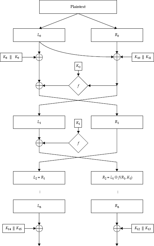
FEAL Algorithm. The basic encryption and decryption algorithm follows a simple Feistel structure, as seen in Figure 4-8. There are several functions that I will cover, but the overall algorithm is as follows:
Calculate a key schedule (K0, K1, ..., K11) in accordance with Section 4.7.4.
Break the plaintext, P, into two 32-bit halves: (L0, R0).
Calculate L0 = L0 ⊉ (K8 || K9).
Calculate R0 = R0 ⊉ (K10 || K11) ⊉ L0.
For r = 1, ..., 8 (i.e., each of eight rounds):
Rr = Lr−1 ⊉ f (Rr−1, Kr−1).
Lr = Rr−1.
Calculate L8 = L8 ⊉ R8 ⊉ (K14, K15).
Calculate R8 = R8 ⊉ (K12, K13).
I will break down the different pieces of these and explain each of them in the following sections.
Rather than use a larger, complicated S-box, a simple function is used in FEAL so that it could be implemented in a few standard computer instructions without requiring large lookup tables. The S-box is called the S-function, defined as a function of three variables: x, y, and δ. Here, x and y are byte values, while δ is a single bit that changes depending on which round the S-function occurs in.
We define S (x, y, δ) as
S (x, y, δ) = rot2(x +y +δ) mod 256
The "mod 256" portion indicates that we need to do simple byte arithmetic. The "rot2" function indicates taking its argument, in this case an 8-bit number, and shifting all of its bits (as seen in its most significant bit form) to the left by two places, with the most significant 2 bits (shifted out on the left) being rotated back in to the least significant bits (on the right). For example:
rot2(00101011) = 10101100
A sample implementation of the S-function, including the rotation function, is shown in Listing 4-6.
Example 4-6. Python code for the FEAL S-function.
########################################### The rot2 function - helper for the S-function##########################################defrot2(x): r = (x < 2) & 0xff# Calculate the left shift, removing extra bitsr = r^(x >>6)# OR in the leftmost two bits onto the rightreturnr########################################### The FEAL S-function##########################################defsbox(x, y, delta):returnrot2((x + y + delta) & 0xff)
The fK function is a helper function that churns the key to create various subkeys.
Here, the inputs to the key generating function, denoted α and β, are 32-bit quantities, split into four 8-bit quantities. Operations are then done with 8-bit arithmetic, probably since, when FEAL was designed, it was much faster than 32-bit arithmetic, and the 8-bit results are recombined into the 32-bit result.
Let the 32-bit result of the key function be referenced by four 8-bit subparts, so that

Let the 32-bit input to fK, α, be referenced as four 8-bit quantities as well: α = α0 || α1 || α2 || α3.
Similarly for β :β = β0 || β1 || β2 || β3.
Calculate

Calculate
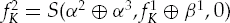
Calculate
Calculate
Recombine the above three results to obtain fK.
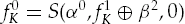
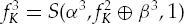
The f-function is the actual round function, acting as the heart of its Feistel structure. It takes as input two 32-bit values (α and β), and produces a 32-bit result.
Split the eventual output of the round function into four separately addressable 8-bit parts:f (α, β) = f0 (α, β) f1 (α, β) f2(α, β) f3(α, β). Call the values it returns simply f0, f1, f2, and f3.
Split the 32-bit input, α, into four 8-bit parts:α = α0 α1 α2 α3.
Do the same for β :β = β0 β1 β2 β3.
Calculate f1 = α1 ⊉ β0 ⊉ α0.
Calculate f2 = α2 ⊉ β1 ⊉ α3.
Recalculate f1 = S (f1, f2, 1).
Recalculate f2 = S (f2, f1, 0).
Calculate f0 = S (α0, f1, 0).
Calculate f3 = S (α3, f2, 1).
To implement these nine steps, we first need to define a few helper functions, to split the 32-bit block into four 8-bit parts (demux) and to recombine 8-bit parts into a single 32-bit block (mux). These are very similar to those used in the SPN cipher above, EASY1. In Python, we can use the code in Listing 4-7.
Example 4-7. Multiplex and demultiplex routines for FEAL.
########################################### Splits a 32-bit block into four 8-bit values# and vice-versa##########################################defdemux(x):# Create an array of size four to store# the resulty = []# Calculate each part in turnforiinrange(0,4):
# They are numbered left to right, 0 to 3# But still in MSB ordery.append((x>> ((3 - i) * 8)) & 0xff)returnydefmux(x):# Initialize result to zeroy = 0# The input, x, is an array of 8-bit valuesforcinx:# Combine each 8-bit value using ORy = (y <<8) ^ creturny
Now that we have all of the helper functions for FEAL, we can define the FEAL main round function, as shown in Listing 4-8.
Example 4-8. The FEAL round function, f.
########################################### Feal round function, f##########################################deff(alpha, beta):# Split alpha and betaa = demux(alpha) b = demux(beta)# Make the output four 8-bit valuesfs = [0,0,0,0]# Calculate each 8-bit valuefs[1] = a[1] ^ b[0] ^ a[0] fs[2] = a[2] ^ b[1] ^ a[3] fs[1] = sbox(fs[1], fs[2], 1) fs[2] = sbox(fs[2], fs[1], 0) fs[0] = sbox(a[0], fs[1], 0) fs[3] = sbox(a[3], fs[2], 1)# Return the 32-bit resultreturnmux(fs)
The key scheduling algorithm for FEAL is meant to split up a 64-bit key into various derived subparts (based on the fK key scheduling function), for use in the main round function of FEAL.
Let K = (A0, B0) and D0 = 0.
For eight rounds, r = 1, ..., 8:
Dr = Ar−1.
Ar = Br−1.
Br = fK (Ar−1, Br−1 ⊉ Dr−1).
In Python, we can implement this fairly easily, as shown in Listing 4-9.
Example 4-9. FEAL key-generating function, fK.
########################################### FEAL key generating function##########################################deffk(alpha, beta):# Split alpha and betaa = demux(alpha) b = demux(beta)# Express output as four 8-bit valuesfs = [0,0,0,0]# Calculate the four 8-bit valuesfs[1] = sbox(a[0] ^ a[1], a[2] ^ a[3] ^ b[0], 1) fs[2] = sbox(a[2] ^ a[3], fs[1] ^ b[1], 0) fs[0] = sbox(a[0], fs[1] ^ b[2], 0) fs[3] = sbox(a[3], fs[2] ^ b[3], 1)returnmux(fs)
Although we will get into more detailed cryptanalysis of FEAL later, there are a few things to note.
It's easy to see that FEAL is almost more complicated than DES: It takes more space to explain and requires more bits and pieces. To give FEAL some credit, most of the operations are indeed very fast: They usually operate on a small number of bits, so that they can be implemented in one machine code instruction.
Blowfish is another Feistel cipher, created by Bruce Schneier in 1994 [14, 15]. According to Schneier, it was designed to be fast, simple, small, and have a variable key [16]. The following description is based mostly on his description in Reference [16].
Blowfish has a slight variant of the Feistel structure previously used and operates on 64-bit blocks. It uses expansive S-boxes and other simple operations. There are two features that differentiate it from DES:
Blowfish's S-boxes are key-dependent — the actual substitution values are regenerated whenever the algorithm is rekeyed. It has four dynamic 8-bit to 32-bit S-boxes.
It has a variable length key, up to 448 bits.
The basic Blowfish algorithm consists of two phases: calculating the key schedule (33,344 bits derived from up to 448 bits of key), and performing the encryption or decryption algorithm.
Schneier refers to the subkeys, generated from the main key, as 18 32-bit keys: P1, P2, ..., P18. The key scheduling algorithm also calculates the S-box, since its values are completely determined by the key itself.
Blowfish Key Scheduling. The P-values and S-box values for the main encryption are calculated based on an input key (of up to a length of 448 bits) and the hexadecimal digits of π.
Initialize the P-values (left-to-right) with the hexadecimal digits of π — that is, the digits to the right of the "hexadecimal point." They start off as
24 3f 6a 88 85 a3 08 d3.... After the P-values are filled, fill the S-boxes, in order with the digits of π. The pre-computed values can be found easily on the Internet.Starting with P1, calculate P1 = P1 ⊉ K1, P2 = P2 ⊉ K2, and so forth. Here, the K-values represent the originally inputted key values, up to 448 bits. There may be up to 14 K-values, to correspond to the P-values. It is necessary to XOR a K-value with each P-value, so repeat the values as necessary by starting over with K1, then K2, and so on, again. For example, with a 128-bit key (representing K1, ..., K4 values), after calculating P4 = P4 ⊉ K4, then perform P5 = P5 ⊉ K1, and so on.
Encrypt a 64-bit block consisting of all zeros (
00 00 00 00 00 00 00 00) using the Blowfish algorithm, with the P-values from the previous step.Replace P1 and P2 with the output from the previous step's Blowfish run.
Take the output from Step 3 and encrypt it (with the new, modified P-values).
Replace P3 and P4 with the output from the previous step.
Repeat this process (encrypting the previous Blowfish output and replacing the next set of P-values), filling all P-values and then the S-boxes (i.e., the 32-bit outputs of the S-box entry) in order. The order of the S-boxes is defined to be S1,0, S1,1, ..., S 1,255, S2,0, S2,1, ..., S 4,255.
This will require a total of 521 iterations in order to compute all values.
The algorithm is based on the Feistel structure, with a total of 16 rounds. The key to the algorithm, as mentioned above, is that the algorithm is kept very simple: For each round, only three XORs, two additions, and four S-box lookups are required.
Blowfish Encryption Algorithm. The basic cryptographic algorithm operates on a 64-bit input and produces a 64-bit output. The following shows the encryption portion. To obtain the decryption code, simply replace Pi in the following with P19−i (with P17 and P18 at the end being replaced with P2 and P1, respectively):
Split the plaintext into two halves: the left half (L0) and the right half (R0).
For each of 16 rounds (i = 1, 2, ..., 16):
Set Li = Li−1 ⊉ Pi.
Set Ri = f (Li) ⊉ Ri.
Swap Li and Ri.
Swap L16 and R16 (undoing the previous swap).
Set R17 = R16 ⊉ P17.
Set L17 = R17 ⊉ P18.
The output is the block obtained by recombining L17 and R17. This main round procedure is shown in Figure 4-9.
The core of the algorithm is, as with all Feistel structures, in the round function.
Blowfish Round Function. In this case, the round function (f in the algorithm) works on a 32-bit argument and produces a 32-bit output by the following method:
Divide the 32-bit argument into four 8-bit values:a, b, c, and d.
Using unsigned arithmetic, calculate S1, a + S2, b. Take the result as a 32-bit integer (ignoring any portion that might have extended beyond 32 bits).
Calculate the XOR of the result of Step 2 and the output of S3, c.
Finally, take the result of Step 3 and add (unsigned, with 32-bit arithmetic, as before) S4, d. This will be the result of the round function.
This round function has a few interesting properties. Notably, which S-boxes are chosen depends on the data themselves: so that the data dictate their own encryption. [This is because the split plaintext (a, b, c, and d) is used to choose the S-boxes.]
The other important note about Blowfish is that it requires 521 encryptions using its own encryption algorithm before it can produce a single block of output. Therefore, encrypting a single block would take very long because of the long setup time. It really only becomes moderately fast to use Blowfish when encrypting at least several hundred blocks (meaning thousands of bits); otherwise, the setup time will dominate the total encryption and decryption times. Luckily, we need to compute the key values and S-boxes only once.
The Rijndael algorithm was chosen by the U.S. Government as the successor to DES [2]. The Rijndael algorithm (and certain parameter settings) was then dubbed the Advanced Encryption Standard (AES).
Rijndael is a variable-sized block cipher named after its inventors, Vincent Rijmen and Joan Daemen. It is a variant of the SPN concept, with more sophisticated and elegant variants of S-box and P-box operations.
Rijndael itself supports block sizes and key sizes of 128, 160, 192, 224, and 256 bits, although AES supports only 128-bit blocks and keys with bit lengths of 128, 192, and 256. The number of rounds for Rijndael varies depending on the key size and the block size. For AES (block size of 128 bits only), the number of rounds is shown in Table 4-4.
The key is, as for most of the ciphers I have been discussing, broken out into a large key schedule, derived from the original key. This is covered in Section 4.9.3.
Rijndael breaks its blocks into a matrix, called the state, with four rows and various numbers of columns (4–8). With block sizes of 128–256, this means that each element of the matrix is an 8-bit value. Figure 4-10 shows an example of this state.
The Rijndael encryption algorithm essentially consists of four basic operations, applied in succession to each other, and looped multiple times:
SubBytes — Each element of the state is run through an S-box.
ShiftRows — The elements of each row of the state are cyclically shifted.
MixColumns — Each column is run through a function to mix up its bits.
AddRoundKey — A portion of the key schedule is XORed with the state.
The AddRoundKey is the only portion of the algorithm dependent on the current round number and the key.
Using the above four pieces, we can specify the Rijndael encryption algorithm.
Table 4-4. The Number of Rounds for Different Values of the Key Length for AES
KEY LENGTH (Nk), IN WORDS | BLOCK SIZE (Nb), IN WORDS | ROUNDS (r) |
|---|---|---|
4 | 4 | 10 |
6 | 4 | 12 |
8 | 4 | 14 |
Here, the values for key length and block size are the number of 32-bit words: Thus "4" corresponds to 128 bits, "6" to 192 bits, and "8" to 256 bits. | ||
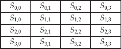
Figure 4-10. A state associated with a 128-bit block size Rijndael, such as in AES. If the state is a 128-bit value, then it it is split into the matrix by breaking it down:S0,0 || S0,1 || S0,2 || S0,3 || S1,0 || S1,1 || S1,2 || S1,3 || S2,0 || S2,1 || S2,2 || S2,3 || S3,0 || S3,1 || S3,2 || S3,3.
Rijndael Encryption Algorithm. Assume that there are r rounds (r is dependent on the key size), and that the plaintext has been loaded into the state.
Run AddRoundKey on the state.
Do the following r − 1 times.
Run SubBytes on the state.
Run ShiftRows on the state.
Run MixColumns on the state.
Run AddRoundKey on the state.
Run SubBytes on the state.
Run ShiftRows on the state.
Run AddRoundKey on the state.
I'll now describe the four sections in a bit more detail. For a more thorough treatment, see References [2] and [7]. The following examples use the details in the AES for a 128-bit block size.
The SubBytes operation essentially functions as an 8-bit S-box, applied to each 8-bit value of the state, as shown in Figure 4-11.

The S-box can be represented in several ways. The normal S-box implementation, with a fixed lookup table, is shown in Figure 4-2. The way I often show it is, if I define the 8-bit input a to be written as a7 || a6 || ··· || a0 and b to be written similarly, then
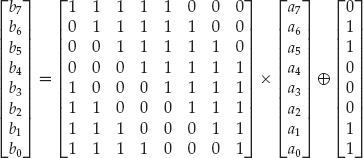
where the × operator means matrix multiplication. If this is confusing, it is fairly easy, and often faster, to just use the lookup-table representation of the S-box.
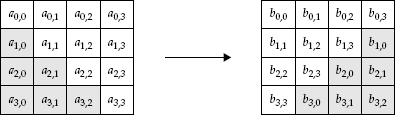
The ShiftRows operation performs a cyclical shift of each row of the state. Each row is shifted by one more value than the previous row (see Figure 4-12):
The first row is left intact (no rotation).
The second row is rotated once to the left.
The third row is rotated twice to the left.
The fourth row is rotated three times to the left.
The MixColumns operation is the most complicated part of the AES algorithm.
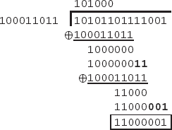
Although I won't go into the nitty-gritty of the mathematics of multiplication over GF(28)(the finite field of size 28, also written as Z2 8), in the case of AES, this essentially means that we will multiply two 8-bit numbers, and take the remainder modulo 283 (which is 100011011 in binary), using binary XOR long
division, not normal arithmetic. This is the same as doing normal division, except that instead of successively subtracting, we use binary XOR. Also, while in normal subtraction, we only subtract if we are dividing a smaller number into a larger number at each stage, whereas with XOR, we only divide if they have the same number of binary digits (so either number can be greater). So that we don't confuse this with normal arithmetic multiplication, I will denote the operation as • (as done in the specification [7]).
For example, I will show how to do this with the AES example in Reference [7], calculating 87 • 131 (or, 01010111 • 10000011). We first multiply the two numbers as usual, obtaining 11,397, or 1010110111001. We then perform the long division to obtain the remainder when divided by 10011011:
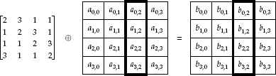
For the MixColumns operation, we are going to take each column and perform a matrix multiplication, where the multiplication is the • operation shown above. The operation will be

where the ai,c entries on the right are the old column entries, the bi,c entries on the left are new column entries, and the ⊗ operator means to perform matrix multiplication with the • operator and XOR instead of addition. We can specify this less abstractly as
b0, c = (2 • a0, c) ⊉ (3 • a1, c) ⊉ a2, c ⊉ a3, c
b1, c = a0, c ⊉ (2 •a1, c) ⊉ (3 • a2, c) ⊉ a3, c
b2, c = a0, c ⊉ a1, c ⊉ (2 •a2, c) ⊉ (3 • a3, c)
b3, c = (3 • a0, c) ⊉ a1, c ⊉ a2, c ⊉ (2 •a3, c)
This operation will be performed for each column, that is, for c = 1, 2, 3, and 4.
The MixColumns operation is shown graphically in Figure 4-13.
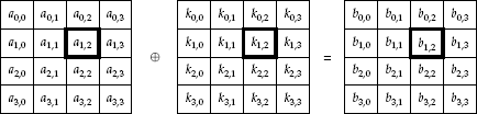
Finally, the AddRoundKey operation takes each 8-bit value of the state and XORs it with an 8-bit value of the key schedule, as shown in Figure 4-14.
Decryption of Rijndael is very similar to encryption: It simply involves doing the operations in reverse (with a reverse key schedule) and using inverse operations for SubBytes, MixColumns, and ShiftRows — these operations are called, surprisingly enough, InvSubBytes, InvMixColumns, and InvShiftRows, respectively.
The use of these inverse functions leads to the following algorithm for decryption:
Rijndael Decryption Algorithm. Assume that there are r rounds (r is dependent on the key size) and that the ciphertext is loaded into the state.
Run AddRoundKey on the state.
Do the following r − 1 times:
Run InvSubBytes on the state.
Run InvShiftRows on the state.
Run InvMixColumns on the state.
Run AddRoundKey on the state.
Run InvSubBytes on the state.
Run InvShiftRows on the state.
Run AddRoundKey on the state.
The most important thing to note is that the keys must be submitted in reverse order.
It is also important to note that the key expansion is changed slightly, as I show in Section 4.9.3.
The inverse operations are fairly easy to derive from the normal ones: We simply construct InvShiftRows by shifting in the opposite direction the appropriate number of times. We construct InvSubBytes by inverting the S-box used (either with the inverse matrix or the inverse of the table). And finally, the InvMixColumns transformation is found by using the following matrix for the multiplication step:
The key expansion step computes the key schedule for use in either encryption or decryption.
Rijndael computes its sizes in terms of 32-bit words. Therefore, in this case, a 128-bit block cipher would have a block size denoted as Nb of 4. The key size is denoted as Nk in a similar manner, so that, for example, a 192-bit key is denoted with Nk = 6. The number of rounds is denoted as r.
Two functions need to be explained in order to describe the key expansion. The SubWord function takes a 32-bit argument, splits it into four 8-bit bytes, computes the S-box transformation from SubBytes on each 8-bit value, and concatenates them back together. The RotWord function takes a 32-bit argument, splits it into four 8-bit bytes, and then rotates left cyclically, replacing each 8-bit value in the word with the 8-bit value that was on the right. Specifically, it computes
RotWord (a3 || a2 || a1 || a0) = a2 || a1 || a0 || a3
Finally, there is a constant matrix that is used, denoted as Rcon. The values of Rcon can be calculated fairly easily using the finite field multiplication operation •. Essentially, the values are calculated as
Rcon (i) = 2i−1 || 0 || 0 || 0
where each of the four parts is an 8-bit number and a member of Rijndael's finite field. Owing to this fact, 2i−1 must be calculated using the • multiplication operator [calculating the previous result times (•) 2], and not normal multiplication. The first few values of 2i−1 are straightforward (starting at i = 1): 1, 2, 4, 8, 16, 32, 64, 128. When we get to 256, though, we need to start using the finite field modulo. Therefore, the next few values are 27, 54, 108, and so on. Table 4-5 shows the required values.
Rijndael is a modern cipher. Since it was created in the late 1990's, after many of the standard cryptanalytic techniques that I discuss in this book were known, it was tested against these techniques. The algorithm was tuned so that it was susceptible to none of the techniques, as they were known at the time.
Although I have limited the discussion to block ciphers up until this point, I should probably have a few words on some of the different ways they are used, besides just straight block-for-block encryption, which has been the assumed method of using the ciphers. (In the previous discussions, I never had the output of one block's encryption affect a different block's encryption.)
The normal method is normally called electronic codebook (ECB). It simply means that each block of plaintext is used as the normal input to the block cipher, and the output of the cipher becomes the block of ciphertext, just as we would expect. Hence, for each block of plaintext, P, we calculate a block of ciphertext by simply applying
C = Encrypt (P)
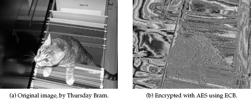
Figure 4-15. A picture of a cat in a filing cabinet, demonstrating the preserved structure present in ECB.
However, there are some issues that can easily arise using a cipher in ECB mode. For example, a lot of the structure of the original data will be preserved, because identical plaintext blocks will always encrypt to identical ciphertext blocks. Figure 4-15 shows how this can occur. In this figure, we encrypt every grayscale (8-bit) pixel (padded with 15 bytes of zeros) with AES in ECB mode, and then take the first byte of the output block as the new grayscale value. (This same method is also used for the CBC example in the next section.)[51]
In general, when identical plaintext blocks always encrypt to identical ciphertext blocks, there is the potential for a problem with block replay : Knowing an important plaintext–ciphertext pair, even without knowing the key, someone can repeatedly send the known ciphertext.
For example, assume that we have a very simple automatic teller machine (ATM), which communicates with a bank to verify if a particular individual is authorized to withdraw cash. We would hope that, at the very least, this communication between the ATM and the bank is encrypted. We might naively implement the above scenario in a simple message from the ATM:
ATM: EncryptK ("Name: John Smith, Account: 12345, Amount: $20")
(Assume that the bank sends back a message saying, "OK, funds withdrawn," or "Sorry, insufficient funds.") The above means simply to send the text message, encrypted with the key K. If the encryption scheme merely represented this as an ASCII message and performed an algorithm, such as AES, using the key K, we might think we are safe, since anyone listening in on the transaction will only see something random, such as
ATM: CF A2 1E C5 AF 67 2D AC 7A E1 0D 3B 2F ...
However, someone could do something sinister even with this. For example, someone listening in on this conversation might simply want to replay the above packet, sending it to the bank. Unless additional security measures are in place, the bank will think that the user is making several more ATM withdrawals, which could eventually drain the victim's bank account.
Even though the ATM used strong encryption to communicate with the bank, it was still susceptible to a block replay attack. Luckily, there are methods to help prevent this attack.
One of the most fundamental ideas of combatting the block replay problem is to make the output of each block depend on the values of the previous blocks. This will make it so that anyone listening to any block in the middle will not be able to repeat that one block over and over again at a later date.
However, simply chaining together the outputs like this still leaves a flaw: It does not prevent block replay of the first block (or the first several blocks, if they are all replayed). A common strategy to fight this is to add an initialization vector (the IV, and sometimes called the "salt") to the algorithm. Essentially, this is a random number that is combined with the first block, usually by XORing them together. The IV must also be specified somehow, by sending it to the other party or having a common scheme for picking them.
Using both of these strategies together results in the simple method called cipher-block chaining (CBC). The method I will describe is taken from Reference [9]. It essentially makes each block dependent on the previous block (with the first block dependent also on the initialization vector). Figure 4-16 shows how this eliminates block replay attacks by ensuring that the same plaintext blocks will be encrypted differently.
CBC Encryption. The following describes the basic CBC method, as described in Reference [9]. The method uses a 64-bit block size for plaintext, ciphertext, and the initialization vector (since the reference originally assumes that DES is used, although any cipher can be used in CBC mode). To adapt it for other ciphers, simply change this to the relevant block size, and use the appropriate algorithm.
Calculate the first block to send by taking the IV and the first block of plaintext, XORing them, and encrypt the result. Hence,
C0 = Encrypt (P0 ⊉ IV)
Calculate each successive block by XORing the previous ciphertext block with the next plaintext block, and encrypting the result. Hence, for i ≥ 1,
Ci = Encrypt (Pi ⊉ Ci−1)
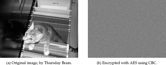
Figure 4-16. A picture of a cat in a filing cabinet. Unlike ECB, CBC obliterates much of the underlying structure.
Decryption in CBC is equally simple.
CBC Decryption. The biggest restriction is that the two users must share the IV or the first block will not be comprehensible to the receiver.
Decrypt the first received ciphertext block, and XOR the result with the IV to obtain the first plaintext. Hence,
P0 = IV ⊉ Decrypt (C0)
For each successive received block, take the received block of ciphertext, run it through decryption, and then XOR it with the previous round's ciphertext to obtain the next plaintext. Hence, for i ≥ 1,
Pi = Ci−1 ⊉ Decrypt (Ci)
There are other issues facing cryptography in addition to block replay. One is padding, or adding additional bits to the end of plaintext so that it is a multiple of the block size. This necessity potentially adds small weakness: We know the last few bits of plaintext if we know the padding scheme. Many ciphers use padding either as all zeros or ones, some other pattern, or perhaps just random bits.
However, the decrypting party needs to know how long the real message is so that any extra padding is thrown away. In some systems, the sending party may not know exactly how long the message is in advance (e.g., it may not have enough buffers to store an entire message of maximum length). In this case, it becomes difficult for the receiving party to know when the message has stopped if padding is used.
In both of these cases, the alternative to using a standard block cipher is to use a stream cipher — one that operates a bit at a time rather than a block at a time. We are mostly concerned with block ciphers in this book, but I shall discuss how block ciphers can be turned into stream ciphers, so that they can operate on one bit at a time (and, therefore, not require padding for any length).
Cipher feedback (CFB) mode is one way to turn any block cipher into a stream cipher, where the stream can consist of any number of bits, for example, it could be a bit stream cipher, a byte stream cipher, or a smaller block size cipher. The following construction is taken from Reference [3].
Assume we are implementing an s-bit CFB mode (with output in chunks of s bits). The only requirement is that s is between 1 and the block size.
CFB works by first encrypting input blocks (the first is an IV) with the key. Then, the "top" (most significant)s bits are extracted from this output, and XORed with the next s bits of the plaintext to produce the ciphertext. These bits of the ciphertext are then sent to the receiver.
At this point, the ciphertext bits are then fed back into the input block, hence the term cipher feedback. The input block is shifted left by s bits, and the ciphertext bits are put in on the right (least significant side). The process is then run again with this new input block.
Output feedback (OFB) mode is very similar to the cipher feedback mode just discussed, and they are often confused.
OFB starts out the same: We have an IV as our initial input block, which we encrypt with the key. Again, we use the most significant bits to XOR against the bits to be output. The result of this XOR is sent out as ciphertext.
Now, the difference is here. Before, we fed back in the ciphertext bits (after XORing with the output).
Instead, we feed back in the output bits of the encryption, before XORing with our plaintext (the result of encrypting the input block). These bits are fed into the bottom of the input block by shifting the block to the right and shifting in the new bits — hence the term output feedback.
The primary difference between these two modes is that the CFB is dependent on the plaintext to create the keystream (the series of bits that are XORed with the plaintext in a stream cipher). With OFB, the keystream is only dependent on the IV and the key itself.
An advantage of using OFB is that if a transmission error occurs, the error will not propagate beyond that corrupted block. None of the following blocks will be damaged by the error; thus, the receiver can recover. With CFB, since the ciphertext is directly put into the input block, the receiving end's incorrect ciphertext value would then be forever sullying the future decrypted bits.
Ciphers can also be operated in counter (CTR) mode, which can also be used to convert them to a stream cipher [3].
A series of counters is used, say, C0, C1, and so on. These counters are normally just increments of one another, hence the term counter. The first counter, C0, should normally be a number that is difficult to guess.
The ciphertext for a given set of plaintext bits is then obtained as follows:
Encrypt the next counter with the key.
Extract the number of bits required, using the most significant bits first. At least one bit will be extracted, and up to all of the bits can be.
XOR the selected bits with the plaintext bits.
The result of the last step is then the ciphertext bits. For the next batch of plaintext bits, encrypt the next counter, and so forth.
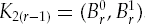
Skipjack [17] is a combination of many different cipher techniques, including large permutations and shift registers. It is a very unique block cipher that operates on 64-bit blocks. It uses an unbalanced Feistel network and an 80-bit key.
Skipjack was designed by the U.S. Government to provide a robust encryption algorithm that enabled law enforcement to decrypt messages through an escrowed key. In other words, the algorithm is designed so that a copy of the key is encoded in such a way that law enforcement could, with an appropriate court order, obtain the key. However, the law enforcement and key escrow portions are not what we are mostly concerned about, but the inner workings of the encryption algorithm itself.
Skipjack is a very unique algorithm, differing in many ways from the traditional Feistel structures and SPNs studied above. For example, many of its operations are in the form of shift registers, rather than straight Feistel or SPN structures, although some of the functions used in the shift registers employ these techniques.
Skipjack's encryption algorithm works fairly simply. There are two rules used in different rounds for a total of 32 rounds.
The plaintext is split into four parts (each being a 16-bit value):
Both rules rely on a permutation, usually written as G. The exact nature of G depends on the round k (since the key mixing is done in the G permutation), so it can also be written as Gk.
Skipjack Rule A. Rule A follows a simple cyclical structure. Note that the counter is incremented every round.
Set the new w1 value to be the G permutation of the old w1, XORed with the old w4 value, as well as the counter.
Set the new w2 value to be the G permutation of the old w1.
Set the new w3 to be the old w2.
Set the new w4 to be the old w3.
Increment the counter.
Figure 4-17 shows this process.
Skipjack Rule B. Rule B works similarly to Rule A.
Set the new w1 value to be the old w4 value.
Set the new w2 value to be the G permutation of the old w1.
Set the new w3 to be the old w1 XORed with the counter and XORed with the old w2 value.
Set the new w4 to be the old w3.
Increment the counter.
Figure 4-18 shows Rule B.
Decryption of a Skipjack ciphertext is fairly straightforward: Every operation from above is reversible, including the G permutation. The rules are replaced with two new rules: A −1 and B −1. The decryption is performed by running Rule B−1 eight times, followed by Rule A−1 eight times, Rule B−1 eight times again, and finally Rule A−1 eight times.
Please note that the counter needs to run backwards. The keys are also submitted in reverse order k = 31, 30, ..., 0. That is, we start knowing the values for k = 32 (this corresponds to the ciphertext) and calculate the values for k = 0 (this corresponds to the plaintext).
Skipjack Rule A−1. Rule A−1 follows a similar structure to Rule A of the encryption.
Set the new w1 value to be the G−1 permutation of the old w2 value.
Set the new w2 value to be the old w3 value.
Set the new w3 to be the old w4.
Set the new w4 to be the old w1, XORed with the old w2 value as well as the counter.
Decrement the counter.
Skipjack Rule B−1. Rule B−1 works similarly to Rule B.
Set the new w1 value to be the G−1 permutation of the old w2 value.
Set the new w2 value to be the counter XORed with the old w3 value, again XORed with the G−1 permutation of the old w2.
Set the new w3 to be the old w4.
Set the new w4 to be the old w1.
Decrement the counter.
The above encryption and decryption relied on functions called the G and G−1 permutations. See Figures 4-19 and 4-20 for their structure.
The F-function is simply an 8-bit S-box. I won't show it here, but it can be viewed in the specifications [17].
Often, we might want to verify that we received the correct message and that nothing is missing or corrupted. One way would be to send the entire message again, but this would double the transmission size, which could be impractical. Naturally, we want this verification message to be as small as possible, while still serving its purpose. This verification message could also be used as a representation of the message itself, if we needed to, for example, prove that we received the message without repeating it in its entirety.

Two constructs that can give us these abilities are message digests and hashes. These calculations provide error detection, smaller representations of data, and sometimes error correction. The representations are called hashes or message digests, since they essentially "chop" up the input and "digest" them into some form.
For error detection and correction purposes, we often see these calculations in the form of checksums and cyclic redundancy checks. These are not designed for most security purposes (such as providing guarantees that the message was not maliciously altered), but simply to provide robustness against transmission or other benign errors; as such, they are usually based on very simple, fast algorithms meant to catch simple errors (such as a single bit being received incorrectly).
![Skipjack inverse Gk transform [Gk]−1.](http://imgdetail.ebookreading.net/career_development/career_development_detail1_2/9780470135938/9780470135938__modern-cryptanalysis-techniques__9780470135938__figs__0420.png)
Hash functions produce hashes from input. These hash functions are designed to provide stronger security than normal checksums: Usually they have complicated, intricate calculations to churn the input to produce output. There are several desirable properties of this in order for the hash to be a secure "representation" of the message:
It should not be easy to obtain information about the input from the hash.
It should not be easy to find two inputs that have the same hash.
It should not be easy to find an input that has a specific hash. Furthermore, it should be even more difficult to find such an input that bears a resemblance to another particular input as well.
Hash functions designed with these security principles in mind are often called cryptographic hash functions.
One primary use for cryptographic hash functions, which require all of the above security, is in digital signatures. As we learned above, performing public key operations can be very time-consuming (such as when taking exponentials of very large integers). These operations become more difficult and time-consuming as the input size increases: To encrypt a 16,384-bit block with an RSA key would require finding primes larger than 16,384, as well as a key, and then performing thousands of arithmetic operations.
A properly designed cryptographic hash can be a representative of the entire input block because of the above properties; there is neither a way to correlate the input and the hash, nor to find similar blocks with the same hash. Hence, we could encrypt the smaller hash using a public-key mechanism.
If a person uses a private key to encrypt the hash of a message, then anyone with the public key can decrypt and verify the hash (since the hash algorithm must be well known). Furthermore, only the holder of the private key could possibly have created the encrypted (signed) hash; thus, we can verify that the message is authentic. This is the essence of a digital signature.
In the following sections I discuss checksums and cyclic redundancy checks and then go into the details of the two most popular hash algorithms: MD5 and SHA-1.
Checksums are very simple measurements of ciphers. Typically, they are implemented with simple arithmetic or bitwise operators, usually addition or XOR.
For example, to calculate an 8-bit additive checksum of a series of bytes, simply add together the bytes and calculate the result modulo 256. For an XOR-based checksum, simply use the bitwise XOR on each of the bytes, which will return an 8-bit value.
Other checksums use similar methods. The key thing to note here is that they are not made for security. They are designed to check for simple errors, such as transmission or transcription errors. Their simple implementation on processors in very few instructions allows them to be used often in communications protocols.
It is fairly easy to defeat a checksum if it is used for security: Either simply modify the checksum itself, or modify a single portion of the message with the appropriate value to make the checksum come out correctly. For example, with an 8-bit XOR checksum, it is necessary to change just one byte to manipulate the checksum to be whatever is desired. Take the current checksum, XOR it with the desired checksum, and XOR this value with any byte in the message. The new message will now have the desired checksum.
A cyclic redundancy check (CRC) is a bit-centric method of error checking that is more robust than normal checksums against many types of errors, but is a tad more difficult to implement.
A CRC takes the original message and does bitwise (XOR-based) long division of it by a fixed, known polynomial. The remainder after the division is then transmitted, which the receiving end can easily verify by also dividing by the fixed polynomial.
CRCs vary in size, with the remainders having bit sizes between 5 and 32 being the most common.
For example, we can calculate a 5-bit CRC of the binary message 011011011 with the 6-bit divisor 101101:
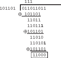
The remainder above is the binary number 11000 (24 in decimal).
MD5 [12] is a message digest algorithm (so named because it was the fifth in a series). It outputs a 128-bit number from any number of bits as input (including zero).
MD5 works fairly simply. First, the input is padded so that its length is equal to 448 modulo 512 (meaning it is 448 + 512 ×n bits long, for any integer n greater than or equal to 0). Then, a 64-bit number representing its length is added to the end of this (or, if the length is more than can be represented in a 64-bit number, then the lower 64 bits of its length). This is appended as the lower-order 32 bits first, and then the upper 32 bits (i.e., in LSB order).
MD5 operates on a 128-bit buffer at a time, split into four 32-bit words, A, B, C, and D. Their initial values are shown in Table 4-6.
Four functions are used in the MD5 computation, one for each major round:
f (x, y, z) = (x &y) | ((¬x) &z)
g (x, y, z) = (x &z) | (y &(¬z))
h (x, y, z) = x ⊉ y ⊉ z
i (x, y, z) = y ⊉ (x | (¬z))
Each of the four portions uses one of these functions 16 times, churning through the data in a fairly twisty manner. At each step of the 64 steps, an
Table 4-6. Initial Values of MD5 Buffer, in Hexadecimal
A: |
|
B: |
|
C: |
|
D: |
|
operation is performed using one of the above functions, followed by a rotation of the bytes:
a = b + ((a +F (b, c, d) + Xk+ Ti) ≪ s)
where F represents the f-function (Steps 0–15), the g-function (Steps 16–31), the h-function (Steps 32–47), and the i-function (Steps 48–63). The Xk-value represents the portion of the message block that we are pulling from. The Ti-value actually represents a value of the sine function, defined to be (from i = 1, ..., 64)
Ti = 232 × abs(sin(i))
Here, we assume that i is the input to the sine function, in radians. (Recall that 2 π radians is the same as 360°.) Finally, we circularly shift left (or rotate left) by different values at each step, represented by the ≪ operation.
After this, we rotate the values:
a′ = d, b′ = a, c′ = b, d′ = c
The values with the prime () indicate the new values to be assigned.
After the 64 steps are completed, the new values for a, b, c, and d, are added into the working hash buffer (A, B, C, D). Then, the next block is loaded, and the process is run again.
See Figure 4-21 for a graphical representation of this.
Finally, the new values are arithmetically added back into the old values (with 32-bit arithmetic):
A = A + a, B = B + b, C = C + c, D = D + d
When the last block is processed, the MD5 signature is the final value of (A, B, C, D).
The Secure Hash Algorithm 1 (SHA-1) [10] is a hashing algorithm specified by NIST that outputs a 160-bit hash.
The following description is based on References [16] and [18].
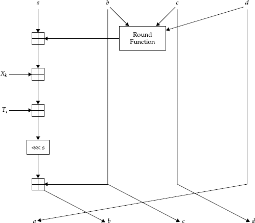
Figure 4-21. Basic round of MD5. Here, the "
SHA-1 takes the input as 512-bit blocks and further splits them into 16 32-bit words, labeled m0 through m15. The words are expanded into 80 such words by the following equation, for i = 16, ..., 79:
mi = (mi−3 ⊉ mi−8 ⊉ mi−14 ⊉ mi−16) ≪ 1
where the ≪ 1 operation rotates the bits, circularly, left by 1.
The initial values of (a0, b0, c0, d0, e0) and (A, B, C, D, E) are
(67452301, efcdab89, 98badcfe, 10325476, c3d2e1f0)
The (A, B, C, D, E) values will represent the hash in the end. For now, we will calculate the (a, b, c, d, e) values and eventually add them when finished processing this block.
There are 80 rounds, for i = 1, ...,80:
ai = (ai−1 ≪ 5) + fi (bi−1, ci−1, di−1) + ei−1 + mi−1 + ki
bi = ai−1
ci = bi−1 ≪ 30
di = ci−1
ei = di−1
The fi functions above change depending on the round:
i = 0, ..., 19 : fi (x, y, z) = (x & y) | (¬x) & z)
i = 20, ..., 39 : fi (x, y, z) = x ⊉ y ⊉ z
i = 40, ..., 59 : fi (x, y, z) = (x & y) | (x &z) |(y &z)
i = 60, ..., 79 : fi (x, y, z) = x ⊉ y ⊉ z
The ki values change depending on the round:
i = 0, ..., 19 : ki = 5a 82 79 99
i = 20, ..., 39 : ki = 6e d9 eb a1
i = 40, ..., 59 : ki = 8f 1b bc dc
i = 60, ..., 79 : ki = ca 62 c1 d6
After we have processed all 80 rounds for the current block, we add the round values (using 32-bit arithmetic) to the ongoing hash values (A = A +a, B = B +b, C = C +c, D = D +d, and E = E +e) and start processing the next block.
Both SHA-1 and MD5 have other "relatives," such as MD4 (similar to MD5, but with a less thorough, and therefore faster, digesting function). However, I shall not discuss them further.
Although we are primarily focused on block ciphers throughout this book, it can be useful to understand a few principles about random number generators in cryptanalysis.
A random number generator is a function that generates a random number: one that cannot be predicted. A true random number generator, one whose output defies prediction, is difficult to obtain. These are normally based on the measurement of some physical phenomenon, which, based on strong scientific support, has no patterns or other characteristics. For example, measuring components of noise and radioactive decay is popular for these numbers.
For these true random number generators, though, there is little to do, cryptanlytically speaking. If the numbers are truly random, no system could produce meaningful results in most cases. One exception to this rule is found in the following section.
Any method for producing random numbers that aren't true is called a pseudorandom number generator.
Even a true random number generator can have a certain flaw: Certain numbers are generated more often than others. For example, although flipping a coin is a fairly random process, there is a very slight, measurable difference in the output numbers generated by the coin toss. This can be due to any number of factors, such as wind, flipping style, and the relative weight of the two sides of the coin. For example, if a coin is flipped 100 times, it may turn out that on average, we can expect heads to occur about 49 times but tails to occur 51 times (with probabilities 0.49 and 0.51, respectively).
This is an example of bias : the characteristic of a process to favor one outcome more often than others, even if that process is truly random.
There are ways to reduce bias, typically by combining several bits to produce one bit, or by combining several sources of randomness with each other. For example, we can simply XOR several bits from different random sources to obtain a new random bit. With the coin example, we will assume that tails is a 0, and heads is a 1. If we take two coin flips, we get a 0 if we have two tails in a row, or two heads in a row, giving us a probability of
The probability of a 1 is therefore 1 − 0.5002 = 0.4998. Both probabilities are much closer to 1/2, giving us a bit that has much less bias in its output (since a purely random coin flip would have a probability of 1/2 for both heads and tails).
Of all of the various types of pseudorandom number generators out there, a decent and popular choice is the linear congruential random number generator [6]. This is a random number generator that gives a sequence of numbers from numbers of the form
X ← (a ×X + c) mod m
This gives a sequence of numbers dependent on integers a, c, m, and the seed, which is the initial value (X0) of the series.
This series is called "linear congruential" because it is based on the fact that the next number is linearly related to the next, modulo m.
Knuth [6] gives some guidance to reduce predictability and bias in this series:
The seed can be chosen arbitrarily. Three common ways to get a seed include saving it between sessions, generating it from the current date and time, or having the user input it. With all of the other variables the same, using the same seed each time allows experiments with a pseudo-random source to be run with repeatable results.
The modulus m should be large, greater than 230. The word size of the computer, such as 32 or 64 bits, is acceptable, especially with speed concerns. But there must be no roundoff errors possible (meaning integer, and not floating point, arithmetic must be used).
If m is the computer word size, such as 232 for a 32-bit computer, then ensure that a ≡ 5 (mod 8). Otherwise, there will be cycles in the output, and certain values will never be hit (because of algebraic properties of linear congruences).
Set a to be in the range m /100 to 99 m/100, and not have a simple digit pattern (like 12121 ...). Furthermore, a should be put through several statistical tests to guarantee that the numbers are acceptable.
Choose c so that it shares no common factors with m, essentially, although its choice is far less important than a. Preferably, do not choose c = 0.
The most significant bits (on the left) are more random than the least significant bits (on the right), and thus these should play a greater role. It's better to use the bits to represent a binary number between 0 and 1, that is, by letting the bits be on the right side after the decimal point (or, better, the "binary point"). Thus, a pseudorandom number generated of 1100 would represent 0.1100 in binary, or 0.75 in decimal. To obtain an integer (say, between 0 and k), multiply by k and truncate. (The natural inclination is to just take the modulus with the higher end of the range, k. This would lead to more biased results, since the least significant digits would be more influential.)
Change a after every m /1000 numbers generated, or so, to keep the numbers from going "stale."
Further guidance on several of these points, as well as how to implement a linear congruential random number generator without floating point arithmetic, can be found in Reference [6].
I'll end this chapter with an idea important to cryptography and cryptanalysis.
Vernam and Mauborgne proposed that, where you have enough key material as you do material to send, and reliable, secure ways to transfer the key material (or some system), then even a simple Vigenère cipher is completely secure [5, 16]. In such a case, a different key could be used for each block for encryption. This system is usually called a one-time pad. (The underlying encryption can be nearly anything, such as a polyalphabetic substitution or simple XOR of the key material with the plaintext.)
The claim of a one-time pad is technically true, but only in the ideal case.
For example, if both parties communicating had a particular book that they would pull key material from, as needed, then they must merely stay synchronized with their material to send messages. The two parties could use the Vigenère Tableau, using letters in words to encrypt the text. It's easy to see that this would completely defeat Kasiski's method, since there are no repetitive patterns of any meaning left.
But, there are three issues: coming up with enough padding material for the one-time pad, synchronizing, and protecting the pad.
Transmitting a lot of information may be very difficult with a one-time pad, because we need one bit of keying material for each bit to be sent. We can't cheat by, say, using a pseudorandom number generator, as above, because there would then be patterns inside the ciphertext that could be exploited. Only a true source of random material that each communicating party can have a copy of will do. In the old days, a large telephone directory or a large book could provide a large set of information to work with (using the letters as keys for a substitution cipher, or deriving bits from the letters for a digital cipher). These aren't truly random, but can be fairly close, depending on how they are used. Today, however, with potentially megabytes, gigabytes, terabytes, petabytes, or even exabytes and beyond needing to be encrypted, the limited amount of information in even these large volumes would be insufficient.
Synchronization is another problem. What happens if a message is lost in transmission when using a one-time pad? Future received messages will then simply start being decrypted as garbage. Sophisticated users of this system could possibly overcome this by using appropriate protocols — for example, once one of the users receives a garbled message, both send the previous message they had sent, starting, say, at the next page whose page number is divisible by 10. This way, they can reset their usage of the key material. However, using even this simple protocol, if it is publicly known, can endanger the cipher, since the adversaries will then know a way to "reset" the cipher to a potentially known pattern.
Finally, protecting the pad is critical: All of the security rests in this one-time pad. The problem is the key distribution problem — how do we transfer this large amount of keying material securely? Furthermore, if we already had this secure channel in place to transmit the very large one-time pad, why can't we just use the same secure channel to send our data? We need a secure channel to establish a secure channel!
While one-time pads are potentially ideal ciphers, their difficulties nearly always make potential users shy away from them and toward different methods, such as using standard ciphers (like DES and AES), with key distribution protocols (like the Diffie-Hellman key distribution protocol).
When studying cryptanalysis, we obviously need something to cryptanalyze. The ciphers in this chapter are popular targets for people to attempt to break because of their widespread use.
Furthermore, cryptanalysis of ciphers can also try to attack some of the other characteristics of ciphers, such as message digests and hashes. Since these are often used as representations of messages, such as in digital signatures, the security of the hash function will then affect the security of the digital signature just as the function used to sign it will. Many of the tools and techniques we develop can be used to also analyze these other constructs.
From here, we are going to explore exactly what we do to start breaking these ciphers.
Exercise 1. Implement MD5 (using Reference [12]), returning only the most significant 24 bits. Use the birthday paradox to find collisions. Try to find many different collisions on many different runs, and calculate the average time to find a collision. Verify that this agrees with the mathematics of Chapter 2.
Exercise 2. Write an implementation of the EASY1cipherinyourprogramming language of choice. (This will be useful in later chapters.)
Exercise 3. Write your own implementation of DES in your programming language of choice. Then, discuss your frustration with the conflicting numbering schemes used in this book and how they differ from the DES specification.
Exercise 4. Write an implementation of AES in your programming language of choice. Compare the running time of encryption in AES and DES.
References
[51] The use of this example (and the CBC that follows) was inspired by the Wikipedia images posted by Lunkwill.
[52] [1] William E. Burr. Data Encryption Standard. In NIST SP 958 – A Century of Excellence in Measurements, Standards, and Technology (2001); http:// nvl.nist.gov/pub/nistpubs/sp958-lide/html/250-253.html.
[53] [2] John Daemen and Vincent Rijmen.The Design of Rijndael: AES – The Advanced Encryption Standard, Information Security and Cryptography. (Springer-Verlag, Berlin, 2002).
[54] [3] Morris Dworkin.Recommendation for Block Cipher Modes of Operation. (National Institute of Standards and Technology, 2001).
[55] [4] Howard M. Heys. A tutorial on linear and differential cryptanalysis. Cryptologia 26 (3): 189–221 (2002).
[56] [5] David Khan. The Codebreakers. (Scribner, New York, 1996).
[57] [6] Donald E. Knuth. The Art of Computer Programming: Seminumerical Algorithms, Vol. 2, 3rd ed. (Addison Wesley, Boston, 1998).
[58] [7] National Institute of Standards and Technology. Federal Information Processing Standard 197: Advanced Encryption Standard (AES). (2001).
[59] [8] National Institute of Standards and Technology. Federal Information Processing Standard 46-3: Data Encryption Standard. (1999).
[60] [9] National Institute of Standards and Technology. Federal Information Processing Standard 81: DES Modes of Operation. (1980).
[61] [10] National Institute of Standards and Technology. Secure Hash Standard. (Federal Information Processing Standards Publication 180-1, 1995).
[62] [11] Rolf Oppliger. Contemporary Cryptography, Computer Security Series. (Artech House, Norwood, MA, 2005).
[63] [12] Ronald L. Rivest. The MD5 Message-Digest Algorithm. (Network Working Group, Request for Comments 1321, 1992).
[64] [13] RSA Laboratories. DES Challenge III. (RSA Laboratories, 1999); http://www.rsa.com/rsalabs/node.asp?id=2108.
[65] [14] Bruce Schneier. The Blowfish Encryption Algorithm. Dr. Dobb's Journal 19 (4): 38–40 (1994).
[66] [15] Bruce Schneier. Description of a new variable-length key, 64-bit block cipher (Blowfish). In Fast Sofware Encryption, Combridge Security Workshop Proceedings, pp. 191–204 (Springer-Verlag, Berlin, 1994).
[67] [16] Bruce Schneier. Applied Cryptography, 2nd ed. (John Wiley, New York, 1995).
[68] [17] U.S. Government. SKIPJACK and KEA Algorithm Specifications. (1998).
[69] [18] Xiaoyun Wang, Yiqun Yin, and Hongbo Yu. Finding collisions in the full SHA-1. In Advances in Cryptology – CRYPTO 2005, (ed. Victor Shoup), pp. 17–36. Lecture Notes in Computer Science, Vol. 3621. (Springer-Verlag, Berlin, 2005).