One Last Random Walk

17.1 Resistor Mathematics

In this discussion I’ll show you a remarkable connection between random walks and electrical resistor networks. It is, at first glance, all too easy to dismiss the mathematics of resistors as trivial, but that would be a very big mistake. To set the stage for the rest of this discussion, then, let me immediately give you an example of the not so obvious ability of resistors to help us understand some very nontrivial mathematics. Consider the inequality

Can you prove that this is so? Also, assuming the inequality is valid, under what conditions does equality hold? Here’s how to answer these questions with resistors.

Consider the two resistor networks in Figure 17.1, where R and R’ are the equivalent resistances between terminals 1 and 2 and 1′ and 2′, respectively. Clearly, the two networks are the same except for the value of the bridge resistor, but the unprimed network “becomes” the primed one if r = 0. Now, let me ask you if you find it “obvious” that R ≥ R′, that is, if one reduces the value of any resistance in a network of resistors (in particular, r > 0 changes to r = 0), then the equivalent resistance must also decrease? The great Scottish mathematical physicist James Clerk Maxwell (1831-1879) thought so, writing in his legendary 1873 A Treatise on Electricity and Magnetism (a work often compared to Newton’s Principia):

Figure 17.1. Resistors prove an inequality

Today this is called Rayleigh’s monotonicity law, and, as Maxwell said, it isn’t hard to prove. But perhaps it is even more self-evident if we draw an analogy between water flowing through a network of pipes and electrons flowing through a network of resistors. As one famous modern book has expressed this,¹ “We just can’t believe that if a water main gets clogged [that] the total rate of flow out of the local reservoir is going to increase.” That is, the water flow (analogous to electrical current) will decrease because the resistance to the flow of water in the now partially clogged network of pipes has increased.

Using the well-known mathematics of resistors in series and in parallel, we can immediately write, for r = ∞,

while for r = 0 we have

By the monotonicity law we must have R ≥ R′, because when writing our two resistance expressions we went from r = ∞ to r = 0. So, we instantly have our inequality. That’s it!

As for when the inequality becomes equality, suppose that

Then the voltages at m₁ and m₂ in Figure 17.1 must be the same (the resistor pairs a and b and c and d are what electrical engineers call a voltage divider). Thus, connecting m₁ and m₂ with any bridging resistance r will have no effect, since the current in r will be zero, because the voltage drop across r is zero. In particular, shorting m₁ and m₂ together, thereby creating the primed network, will have no effect.

Can you show, analytically, that equality results for the given condition, without making any reference to resistors and voltage dividers? (Fair warning: this can be a bit tricky, which is why you’ll see this question again, at the end of this discussion, as a challenge problem.) Of course, without the resistor circuits to guide us, I don’t think it would be at all evident what supposed condition for equality we should even try.

17.2 Electric Walks

Okay, down to business. Consider an arbitrary network of resistors, as shown in Figure 17.2, with any pair of nodes either not connected or, if connected, connected by a single resistor. (If two connected nodes are joined by multiple resistors in parallel, just replace them with their parallel equivalent. Resistors in series means, of course, that one or more additional nodes must be included in the set of all nodes.) Two particular nodes, labeled A and B, are connected to the terminals of an ideal (that is, zero internal resistance) one-volt source. If V_x is the voltage at node x, then in particular we write VA = 1 and V_B = 0.

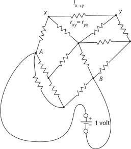
Figure 17.2. An arbitrary resistor network.

Now, consider two nodes, x and y, connected by the resistor r_xy(which of course equals r_yx). There are, in fact, possibly multiple nodes connected to node x, and so node y is just one of perhaps many (in Figure 17.2 there are three nodes connected to node x). Let’s write N(x) as the set of all nodes connected to node x, and since y is a member of that set, I’ll write y ∈ N(x).³ We can write Kirchhoff’s current law for the total current out of node x and into all the nodes that x is connected to as

Next, let’s make the definition

where we know, physically, that C_x ≠ 0.⁴ This allows us to write

or

and so, finally, since c_x ≠ 0,

which is the result of a purely electrical physics analysis. Let’s put (17.3) to one side for the present and start all over again with a second, purely mathematical analysis.

I’ll start by first asking you to forget, just for now, all about electrical current being electrons moving through conductors because of forces acting on them from the electric fields produced by a voltage source. Now our typical conduction electron is to simply be imagined as a random walker moving node to node to …, with each node transition to be made according to the following rule:

The choice of which of the nodes y ε N(x) to move to is purely mathematical in nature, to be made randomly and independently of all the earlier node transitions the electron may have made; notice that now there is no electrical engineering tech talk of fields or forces. All we have are electrons wandering randomly, just like the hiker in Frost’s poem, through a wood of nodes. Notice, too, that if we sum the probabilities of (17.4) over all possible y, we get

which becomes, from (17.2),

This is the mathematics saying our wandering electron goes from node x to some other node y with certainty. The fact that all the transition probabilities sum to unity means that the electron always does move, and doesn’t have a non-zero probability of remaining at node x.

Now, here’s where all this is going. Let’s define N_x as the probability that our electron, if at node x, will reach node A before reaching node B. Then,

We can multiply probabilities this way because of the assumed independence of the node-to-node transitions. That is,

or, using (17.4),

Have you noticed that (17.3) and (17.5) are the same if we take N_x = V_x? That is, the probabilities N_x are numerically equal to the node voltages V_x! This probabilistic interpretation of the node voltages makes obvious sense, too, in the two special cases of node x as either A or B. That is,

which says starting at A, our electron will reach A before B with probability one (undeniably true), and

which says starting at B, our electron will reach A before B with probability zero (who would deny that?).

The two equations (17.2) and (17.4), as simple as they appear, are the basis for an incredible new way to “solve” dc resistor networks. To find the voltage at any node of the network, all we have to do is start a random walk at the node of interest, and then “decide” to which connected node to move. The “decision” is made by what amounts to the old children’s party game of spin the bottle (which girl to kiss becomes which node to move to), with the node transition probabilities being given by (17.2) and (17.4). The walk continues until it reaches either A or B, with either condition terminating the walk. This is certain to happen eventually, although because of the randomness in the node-to-node transitions, it isn’t a priori clear just how long it may take. It is perfectly possible, after all, for our random-walking electron to spend time simply bouncing back and forth between a pair of connected nodes. In practice, however, the entire process runs to completion on a computer very quickly. If we do this many times, all the while keeping track of how many walks terminate because they reached A, then we can estimate the probability of reaching A before B if the walk starts from the node of interest. But that probability is the voltage of the node of interest.

If we repeat the above for each of the nodes in the network (other than A or B, of course, the voltages of which we know from the start), then we’ll have a complete solution to the circuit. If the actual input voltage for your circuit is different from one volt, then use the linearity of resistors to simply scale the one-volt solution up (or down) to get the node voltages for your circuit. And remember, at no time have we used the concepts of electric fields, forces, or moving electrons as electric current.

17.3 Monte Carlo Circuit Simulation

It is one thing to say (17.2) and (17.4) allow the Monte Carlo simulation of resistor circuits and quite another to actually produce a computer code that does the job. It’s not that it is necessarily difficult to write such a code, just that it’s hard to find a published code. More common is to find references to such codes, with only their results for particular circuits published. For example, in one paper⁵ we are told of a code written in BASIC, specifically for the Wheatstone bridge circuit,⁶ that “requires less than a page of code.” Alas, the code itself was not presented. The author did say he would send a copy of his code to anyone who asked for it, but that was twenty years ago, and anyway, BASIC isn’t the scientific programming language of choice any longer (if it ever was). We are told, however, that using “100 walks gives the exact answer … to about 10% accuracy and 10, 000 walks are needed for 1% precision. The 1% result requires only about a minute on a personal computer.” A million walks should give about 0.1% accuracy.

So, here I’ll show you how to write a MATLAB code that will solve any resistor circuit, not just a specific one. Further, it will use millions of random walks, and yet, even for circuits much more complicated than a Wheatstone bridge, it will require only a few seconds to run. (Of course, my 2007—when I’m writing this—personal computer is almost surely vastly more powerful than any 1990 machine was.) And finally, my MATLAB code will “require [almost] less than a page.” Here it is, the code mccube.m. What follows after the code is how the code works.

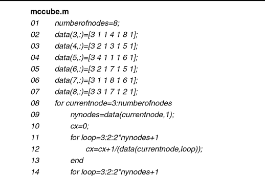
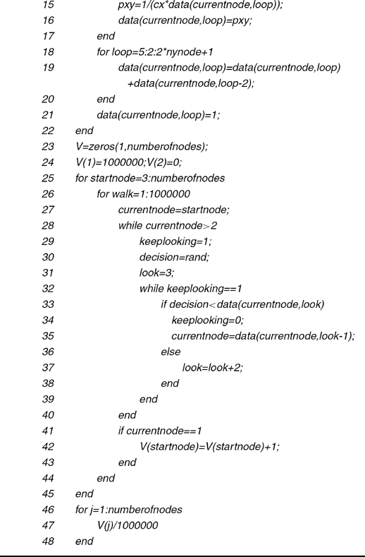
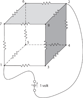
Figure 17.3. A 3-D resistor cube.

The hardest part of writing a circuit code is, I think, the development of a means by which to “tell” the code the topology of the circuit. That is, how do we tell a computer which nodes are connected to which nodes, and the values of the connecting resistors? There may be as many different ways to do that as there are analysts, but the method I used is quite simple and direct. I will be imposing the constraint that the nodes of the circuit be numbered sequentially from 1 (because MATLAB doesn’t allow zero indexing of vectors and arrays), where node 1 is always the positive terminal of the voltage source (one volt) and node 2 is always the negative terminal of the voltage source (zero volts). Then all the other nodes are numbered, in any arbitrary order you wish, from 3. To be very specific, let’s suppose our circuit is a three-dimensional cube of one-ohm resistors (hence the name mccube.m, for Monte Carlo cube, although the code will run any other resistor circuit just as well), as shown in Figure 17.3, where I’ve labeled each node with an integer running from 1 to 8. Our goal is to find the voltages at nodes 3 through 8.

This problem is a classic, a favorite on master’s and even PhD oral exams, because electrical engineering and physics professors know the easy way to analyze it, while most examinees—who are already in a state of nervous shock—immediately attempt to write Kirchhoff’s equations for the cube and make a botch of it. It is something (unkind?) professors do because their professors did it to them!

Figure 17.4. A row vector in the topology matrix data

The heart of mccube.m is the matrix data. Every node in whatever circuit we are going to study has a row in data. The general format of a row is shown in Figure 17.4, where data(i,:) is MATLAB’s way of specifying the ith row (node i). The colon as the second index simply means we are talking of the entire row, not of an individual element in the row. The very first thing the code needs is the value of the variable numberofnodes (see line 01), which, as you have no doubt guessed, is the number of nodes in the circuit, including the voltage source nodes 1 and 2. In mccube.m this variable receives the value of 8 for the 3-D resistor cube. Then in lines 02 through 07, the rows of data are specified in the format of Figure 17.4. For example, line 02 says node 3 connects to three other nodes: to node 1 through a one-ohm resistor, to node 4 through a one-ohm resistor, and to node 8 through a one-ohm resistor. The rows for nodes 1 and 2 are not needed, since we are not going to launch any random walks from those nodes (we already know the voltages at those two nodes).⁷

Lines 08 through 22 then transform the topology matrix data into a probability transition matrix, using equations (17.2) and (17.4). What that means is the i th row of data will, when those lines of code have done their job, no longer specify the resistances through which node i is connected to other nodes; rather, the elements in data where the resistance values were will now contain numbers that determine the probabilities that random walker at node i will move to each of those other nodes. Because of the way I wrote the random walk section of the code (to be explained momentarily), these numbers are not the actual node transition probabilities but rather are cumulative probabilities. For example, the new row in data for node 3 will have become

In the random walk portion of the code (lines 25 through 45) the variable decision is given a random value from 0 to 1 (line 30) and then the code sequentially uses decision to decide to which node to go to next. If, for example, the walk is currently at node 3 (currentnode=3) then data(3,:) says to go to node 1 if decision<0.3333, but if not then go to node 4 if decision<0.6666, but if not then go to node 8 (decision<1 is certain to occur at this point and that will be the case with a priori probability 0.3333 (I’m ignoring any roundoff error here, of course, a concern addressed in particular by line 21).

Line 23 defines the row vector V of length numberofnodes. V(i) will, when the code finishes, be an estimate of the voltage at node i. The random walk algorithm, you’ll recall, keeps track of how many times (out of one million walks) a walk starting from node i reaches node 1 before it reaches node 2. These numbers are stored in the vector V. To convert these numbers to probabilities (and, hence, to voltages) we simple divide by one million. That’s why V(1) and V(2) are initially set (in line 24) to 1, 000, 000 and 0, respectively, since we know the voltages at node 1 and at node 2 are one volt and zero volts, respectively.

The random walk portion of the code is line 25 through line 45 and is, I think, pretty transparent; just keep the format of the data probability transition matrix in mind. An individual random walk, beginning at startnode (which itself will run from 3 to numberofnodes—see line 25), continues until line 28 determines a walk has reached either node 1 or node 2 (all other node numbers are of course greater than 2). Lines 41 through 45 determine which it is and, if it is node 1 then V(startnode) is incremented by one. A million such walks are launched from every node from 3 to numberofnodes. Finally, lines 46, 47, and 48 print the node voltage estimates.

So, at last, the big question: how well does mccube.m perform? To answer that, we need the actual node voltage values of the resistor cube to compare with the code’s estimates. To get those exact values, let me now show you the easy way I mentioned earlier to analyze the 3-D resistor cube. To start, imagine that rather than a one-volt source connected to nodes 1 and 2, we have adjusted the voltage to be whatever it has to be so that the source current is one ampere. If we write I_x→y as the current flowing from node x to node y, as we did in (17.1), then by symmetry the source current splits equally at node 1, and so

Further, and again by symmetry,

One can make the same argument for I_7→6 and I_7→8, too, that is

and so, too,

Now, in particular

Thus, the voltage drop from node 1 to node 2 is

(drop from 1 to 7) + (drop from 7 to 6) + (drop from 6 to 2)

because all of the currents are in one ohm resistors.

To summarize: a voltage source of 5/6 volts causes a one ampere source current. So, linearly scaling (resistors are linear) we see that a one-volt source would result in a source current of 6/5 A. Again using the current splitting symmetry argument, we see that there is a current from node 1 to node 7 of

which means there is a voltage drop of 2/5 = 0.4 volts from node 1 to node 7 (and from node 1 to nodes 3 and 5, as well). Thus,

Further, that 2/5 A current flowing into node 7 splits (by symmetry) evenly, and so there is a current of 1/5 A flowing from node 7 to node 8. This gives an additional voltage drop of 1/5 = 0.2 volts from node 7 to node 8, and therefore

The following table sums all this up, as well as giving mccube.m’s results, to four decimal places. The agreement is really pretty good; the execution time was less than six seconds.

As a quick second example, consider the “pinwheel” circuit of Figure 17.5. It is not difficult to show⁸ that the node voltage values are

To input this circuit to the computer simulation code, all that is required is the modification of lines 01 through 06 to read

as well as, of course, deleting line 07. In a bit less than three seconds the code produced the node voltage estimates

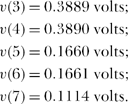
Again, we have pretty good agreement with theory.

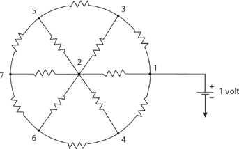
Figure 17.5. A pinwheel of resistors.

17.4 Symmetry, Superposition, and Resistor Circuits

Our “easy” solution of the 3-D resistor cube depended totally on the high degree of symmetry displayed by the cube and its connections to the voltage source. This no doubt accounts for much of the appeal of that problem to analysts, who generally place arguments based on symmetry high on their list of “beautiful” arguments.⁹ The concept of superposition ranks high on that list as well, and there is another famous resistor circuit problem that requires both concepts. This problem, which has been a favorite of electrical engineering and physics professors since its appearance in 1950,¹⁰ is based on the infinite, two-dimensional square network of one-ohm resistors shown in Figure 17.6. The question is easy to state: what is the resistance between nodes A and B? The answer is certainly less than one ohm, but how do you account exactly for the infinity of resistors around the resistor that directly connects A and B?

Figure 17.6. An infinite square grid of resistors.

The “easy” solution to this problem requires three simple, sequential steps.

Step 1: Imagine a one-ampere current source that injects current into the grid at node A. The current exits the grid along its “edge at infinity” (use your imagination with this!). By symmetry, the one ampere into A moves away from A by first splitting equally into four 1/4-ampere currents, one of which flows from A to B. This results in a 1/4-volt drop from A to B.

Step 2: Remove the one-ampere current source of Step 1 and hook another one up to the grid so that it injects current into the grid at infinity and removes it from the grid at node B. By symmetry, the one ampere removed at B flows into B as four 1/4-ampere currents, one of which is flowing from A to B. This results in a 1/4-volt drop from A to B, with the same polarity as in Step 1. (Important observation: we are, in Steps 1 and 2, treating both A and B as the “center” of the grid, and, since the grid is infinite in extent, we can do that; indeed, any node in an infinite grid can be thought of as the “center”).

Step 3: Finally, leaving the one-ampere current source of Step 2 in place, reconnect the original one-ampere current source of Step 1 that injects current into node A. Then, by superposition, we can add the effects of the two currents when individually applied to get their combined effect when both are in place at the same time. That is, we have one ampere into A, one ampere out of B, zero current at infinity, and a total voltage drop of 1/4 + 1/4 = 1/2 volt from A to B. So, 1/2 volt “causes” one ampere of current (or vice versa, if you wish), and therefore the resistance between A and B is 1/2 ohm. That’s it!

This elegant solution did not appear along with the original 1950 statement of the infinite square grid of resistors, but rather in the solution manual to a 1966 physics textbook.¹¹ But this elegant solution works only because of the very high degree of symmetry in the problem. The original 1950 presentation actually solved the far more general problem of calculating the resistance between nodes A and B when A and B could be any pair of nodes in the infinite grid, not just adjacent ones. For example, if A and B are diagonally opposite nodes of one of the squares of the grid—that is, if A’s coordinates are (0,0) and B’s are (1,1)—then the resistance between A and B was given as 2/π ohms. If we call R_m,n the resistance between nodes (0,0) and (m,n)—and so in the “easy” symmetrical case we analyzed earlier we have ohm—then the 1950 book gives the “Knight’s move” resistance as ohms. Something of a puzzle still remained after 1950, however, because that solution involved the evaluation of a number of difficult integrations, and no discussion of how they were done was given.¹²

In 1972 Leo Lavatelli (1917-1998), a physicist at the University of Illinois, gave a beautiful derivation¹³ of the 2/π result using only algebra and trigonometry. Thirteen years later the English mathematician Peter Trier (1919-2005) used two-dimensional Fourier series to express R_m,n as a double integral.¹⁴ Almost a decade later (1994) Giulio Venezian, a physicist at Southeast Missouri State University, gave an explicit solution for the resistance between any two nodes of an infinite square grid of resistors in terms of one-dimensional integrals, and numerically evaluated them.¹⁵ While Venezian’s integrals don’t look anything at all like the ones in the 1950 book (evaluated, as I’ve said, analytically by unexplained means), Venezian’s results are in agreement. For example, Venezian’s numerical integrations result in R1,2 = 0.773 ohms. The 1950 book gave the expressions for all R₀=m≤3,0≤n3, while Venezian’s numerical values are for R₀≤m≤10,0≤n≤10. By physical symmetry, we have R_±m,±n = R_m,n, m,n ≥0,and R_m,n = R_n,m, which can be mathematically seen in Trier’s double integral (see note 14 again).

Five years after Venezian’s paper, another paper¹⁶ appeared that, using Venezian’s method, extended the original 2-D infinite resistor grid to 3-D and higher-dimensional infinite cubic lattices, as well as giving explicit evaluations of the resulting integrals in analytical form, using the powerful symbolic manipulation capability of the computer application Mathematica. The authors’ code confirmed the known expressions and computer-generated expressions for were given—for example, that = 0.991924… ohms and that = 1.076379 … ohms, both in excellent agreement with Venezian’s numerical evaluations.

CP. 17.1:

Show, analytically, that

if

CP. P17.2:

Consider again the infinite square grid of one-ohm resistors shown in Figure 17.6, but with the resistor joining nodes A and B removed. What then is the resistance between A and B?

CP. P17.3:

Take a look again, if you didn’t solve it before, at CP. 3.5.

CP. P17.4:

In Discussion 3 you saw several examples of the analytical difficulties that an infinite number of resistors can cause. Here I’ll illustrate for you how just one resistor can do the same. If we have a one-ohm resistor carrying current i(t), then the instantaneous power is p(t) = i²(t), and the total energy dissipated (as heat) by the resistor is then given by And finally, by definition the current i(t) is the rate at which electrical charge moves through the resistor, that is, , and so the total charge that passes through the resistor is All this is just standard first-year electrical physics. Now, let’s consider a specific i(t). For c a positive constant, define

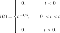
That is, i(t) is a finite-valued pulse that is zero except for a finite length of time. The total charge transported through the resistor is

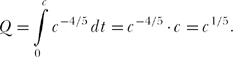
Suppose now that we pick the value of c to be ever smaller, that is, we let c → 0. Then the pulse-like current becomes ever briefer in duration and ever larger in amplitude. At the same time, lim_{c→0 Q(t)} =. And finally, since i²(t) = c^−8/5 during the time when the pulse amplitude is non-zero, the dissipated energy which means the resistor should instantly vaporize because it’s dissipating infinite energy in zero time! But how can that be, since in the limit as C→0 there is no charge transported through the resistor?

Notes and References

1. You can find Maxwell’s words on p. 427 of volume 1 of the Treatise.

2. The quote is from Peter G. Doyle and J. Laurie Snell, Random Walks and Electric Networks (Carus Mathematical Monograph 22; Washington, D.C.: American Mathematical Association of America, 1984, p. 70). This seminal work includes an elegant discussion of Rayleigh’s (this is the same Rayleigh who appeared in Discussion 14) monotonicity law—first stated by Rayleigh in 1871—in its Chapter 4. If you look back at the discussion about calculating the input resistance to the infinite circuit of Figure 3.9c, you’ll see I’ve already invoked Rayleigh’s monotonicity law in this book without calling it that.

3. Here I am following the notation of Monwhea Jeng, “Random Walks and Effective Resistances on Toroidal and Cylindrical Grids” (American Journal of Physics, January 2000, pp. 37-40).

4. This follows from the observation that c_x = 0 would require that every r_xy in (17.2) be infinite. But that would mean nodes x and node y are really not connected, contrary to assumption.

5. Raymond A. Sorensen, “The Random Walk Method for DC Circuit Analysis” (American Journal of Physics, November 1990, pp. 1056-1059).

6. The Wheatstone bridge—named for the English scientist Charles Wheatstone (1802-1875) who, in fact did not invent the circuit and freely admitted so—is a circuit for very accurately measuring the value of an unknown impedance. You can find its theory developed in any good electrical engineering or physics text that discusses electrical circuits.

7. Since data is a matrix, MATLAB requires all the rows of data to have the same length. Because all the nodes in a 3-D resistor cube each connect to the same number of other nodes, this requirement is automatically satisfied by this particular circuit. In circuits where that is not the case, however, all the shorter rows in data must be “padded out” with zeros to have their lengths equal that of the longest row. This keeps MATLAB happy, although the Monte Carlo code never actually looks at those padding zeros.

8. See my paper “A Simple Operator Approach for Analytic Solution of Linear Constant-Coefficient Difference Equations” (IEEE Transactions on Education, December 1968, pp. 234-239).

9. Here’s a very pretty application of symmetry from pure mathematics. If you look in any good set of math tables you’ll find the following definite integral: . This holds for any real value of m, for example, m =−π,0 (this special case should be obvious!) and 11 073 642 07. How in the world, you might fairly ask, can such a wonderful result be established? If you try to prove it using any of the usual methods discussed in freshman calculus, then I think you’ll find it a frustrating task. With symmetry, however, it’s actually easy. In Figure 17.7 I’ve plotted the behavior of the integrand over the interval 0 to p/2 for two values ofm picked at random, one negative and one positive (−π/3 and ), and from those two curves, you might reasonably guess that the plots for any value of m will be symmetrical around the point (. If that is so, then clearly the integrand divides the area of the box (equal to π/2) in half, and since the half that is beneath the integrand curve is the integral, then we immediately have our result! The symmetry for any m is easily established by noticing that, if true, it follows that if we write f(x) for the integrand, then what we mean by saying f(x) is symmetrical around ( is just that f(x) = 1 — that is, f(x) + for every value of x in the integration interval 0 to π/2. And, in fact, this is so because That’s it! Symmetry, and the area interpretation of integration, are all we have used to show that for any real m.

Figure 17.7. Symmetrical integrands.

10. B. van der Pol and H. Bremmer, Operational Calculus (Cambridge: Cambridge University Press, 1950 [2nd ed. 1955], pp. 371-372). The authors tell us in the book’s opening that much of their writing was done during the Nazi occupation of the Netherlands during World War 2. Logic in the midst of madness.

11. E. M. Purcell, in the solutions manual for his book Electricity and Magnetism (New York: McGraw-Hill, 1966).

12. The integrals in the 1950 book are

I think just about everybody would disagree with the authors in note 10 who claimed this incredible integral can be “simply calculated” for given values of m and n. How they did it remains, I believe, a mystery to this day.

13. Leo Lavatelli, “The Resistive Net and Finite-Difference Equations” (American Journal of Physics, September 1972, pp. 1246-1257). An earlier paper extended the symmetry/superposition argument to other infinite, non-square resistor grids (triangular and honeycomb, for example) but was still limited to A and B being adjacent nodes; see Francis J. Bartis, “Let’s Analyze the Resistance Lattice” (American Journal of Physics, April 1967, pp. 354-355).

14. P. E. Trier, “An Electrical Resistance Network and Its Mathematical Undercurrents” (Bulletin of the Institute of Mathematics and Its Applications, March/April 1985, pp. 58-60). Trier’s double integral is the very pretty

which clearly displays the symmetry R_m,n = R_n,m. Compare this expression for R_m,n with the one in note 12.

15. Giulio Venezian, “On the Resistance Between Two Points on a Grid” (American Journal of Physics, November 1994, pp. 1000-1004).

16. D. Atkinson and F. J. van Steenwijk, “Infinite Resistive Lattices” (American Journal of Physics, June 1999, pp. 486-492).