Nearest Neighbors

16.1 Cannibals Can Be Fun!

Well, with an opening like the one above you may be wondering if your author has himself been driven around the bend with all the random walks and MATLAB coding we’ve been doing. Actually, there is one more random walk I want to show you, with a totally unexpected application to physics, but I’ll defer that until the next discussion. Here we’ll take a break from random walks but still keep our feet in probability (and just a bit of MATLAB, too). Discussing the nearest neighbor problem in terms of cannibals is simply for fun, of course, but similar mathematical problems regularly occur in physics, for example, in astrophysics when discussing the distribution of stars in space, and I’ll say just a bit more on that in the brief final section of this discussion. For now, though, back to cannibals.

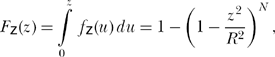
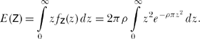
Imagine N + 1 cannibals who are randomly and independently scattered about a circular island with radius R.(WhatImeanby random is just this: when each cannibal is positioned on the island, he or she is as likely to be in the middle of one little patch of area as in any other little patch of area of the same size.) One of the cannibals happens to be at the exact center of the island, and I’ll name him H (for hungry). H is a trained mathematician (culinary preferences having, of course, nothing to do with intellectual capability) who is interested in computing the average distance separating himself from the nearest of his N neighbors, whom of course H would like to have “join him for lunch.” To calculate that average distance, H decides to first find the probability density function (pdf) of the random variable Z, which represents the distance from H to his nearest neighbor (Z’s values are in the interval 0 to R). If we call this pdf f_z(z), then the average value of Z (also called the expected value of Z and written as E(Z)) is given by

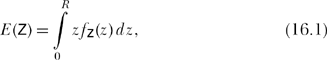
a formula derived in any elementary textbook on probability theory. Remember what f_z(z) means:

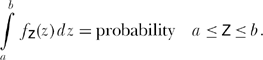
Here’s how to easily derive f_z(z). Imagine a circle of radius z centered on H. The probability that any individual one of H’s neighbors is inside that circle (that is, the probability that that particular neighbor is no more than distance z from H)—because of the above area interpretation of what random means—is given by

It follows that the probability that that neighbor is more than distance z from H is

Theprobability, then, that none of H’s N neighbors is within distance z of H (that is, all of H’s neighbors are more than distance z away) is given (because of the given independence of the cannibals’ locations) by

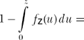
This is, in other words, the probability that H’s nearest neighbor is more than distance z from H. Since

probability H’s nearest neighbor is within distance z of H, then

probability H’s nearest neighbor is not within distance z of H,

or, from (16.2),

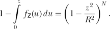
Thus,

where is the distribution function of z. To solve for the density fz(z) we differentiate the distribution¹ with respect to z to get

or

Figure 16.1 shows what the pdfs for some selected values of N look like for the case of R = 1.

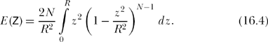
Putting (16.3) into (16.1),

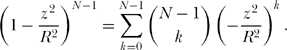
We can perform the integration as follows, with the aid of the binomial theorem. From high school algebra we have the wonderful identity

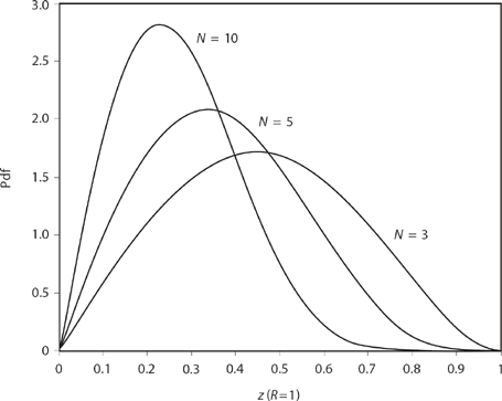
Figure 16.1. Some nearest neighbor pdfs.

or, if we set x = 1,y = − z²/R², and n = N — 1, we can write

Thus,

or

Inserting (16.5) into (16.4),

or, as

then

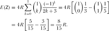
We can easily evaluate (16.6), either by hand or by writing a simple computer routine. For example, for N = 1 we have

a result that sometimes surprises people who expect it to be ½ R. And for N = 2 we have

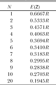
The following table shows the behavior of E (Z) as a function of N; E(Z) monotonically decreases with increasing N, as you might expect, but perhaps not as fast as you might think before doing this analysis.

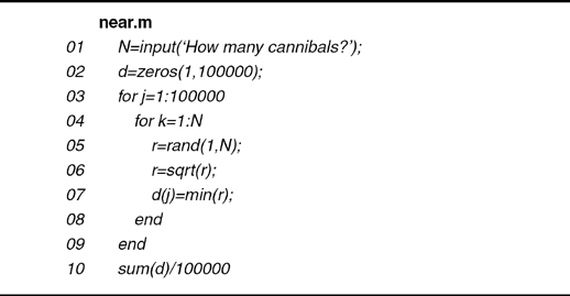
We can “experimentally” check these calculations by performing a Monte Carlo computer simulation. That is, let’s perform, say 100,000 times, the random placement of N cannibals inside a circle followed by the determination of the distance from H—at the circle’s center—of that cannibal closest to H. An average of those 100,000 minimum values ought to give us a pretty good approximation to E(Z), for a given N. To write the code that does this, however, requires a procedure that randomly picks N points uniformly distributed over the circle. One easy way to do this is to assume (with no loss of generality) that R = 1, and to then generate N random numbers uniformly distributed from 0 to 1, and then to take their square roots.² The following very simple MATLAB code near.m does the job, where all the commands should

be transparent with the following explanations: line 02 creates a row vector d with 100,000 elements; line 05 creates a row vector r of N random numbers uniformly distributed from 0 to 1 (and then line 06 replaces that vector with a vector whose elements are the square roots of the original vector’s elements; line 07 stores the smallest element in the square root vector r in the current element (index j)ofthe d vector; line 10 sums all the elements of the d vector and divides by 100,000, that is, computes the average of the values stored in the elements of the d vector.

When run, near.m produced the following table of estimates for E (Z) versus N.

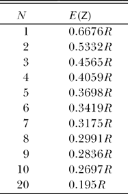
Comparing this table with the previous one based on (16.6), you can see that the agreement between theory and “experiment” is pretty good.

16.2 Neighbors Beyond the Nearest

What of H’s second nearest neighbor, or his third one, or, indeed, his ith nearest neighbor? If, for example, the second nearest neighbor is a tastier possibility than the nearest neighbor, and if that second nearest neighbor isn’t too much more distant, maybe it would be worth the extra travel distance! To work out the probability density functions for all these cases turns out, remarkably, to not be difficult at all (although perhaps just a bit tricky). This more general question should, of course, contain our earlier results as the special case for i = 1.

Let Q(z) be the probability an individual cannibal is within distance z of H, which we know from the previous discussion is given by

Then, the probability that exactly k of his N neighbor cannibals are within distance z of H is given by the binomial probability law as

Now, if the ith nearest neighbor is within distance z of H, then i or more neighbors are within distance z of H (if the ith nearest neighbor is within distance z, then i — 1 even nearer neighbors certainly are too, as well as perhaps one or more additional neighbors, all the way up to possibly all the neighbors). Thus, the total probability that the ith nearest neighbor is within distance z of H is given by

Clearly, NN_i(z) is a distribution function, that is, NN_i(z) = Prob(distance from H of his ith nearest neighbor ≤ z), and so the pdf of the distance of H’s ith nearest neighbor is

Thus,

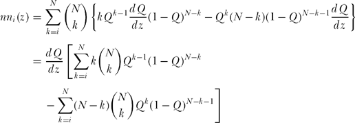
or, explicitly writing out the first term of the first summation,

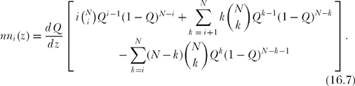
In the second summation of (16.7), when k = N the final term is zero, and so

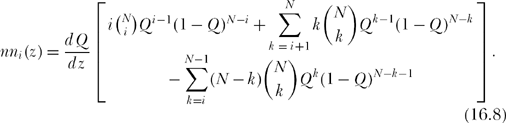
In the first summation of (16.8) change index to j = k — 1, that is, k = j + 1. Then,

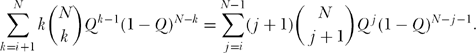
Now, notice that

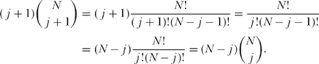
So,

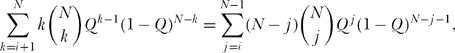
but this is precisely the second summation in (16.8)! That is, the two sums in (16.8) cancel—this is, I think, a fantastic gift from the number gods—and we are left with the astonishingly simple result that the pdf of the random variable for the distance to H’s ith nearest neighbor is

or, since Q(z) = z²/R²,

The pdfs in (16.9) are near neighbor pdfs. If i = 1, then we are back to our original nearest neighbor pdf, and (16.9) reduces to

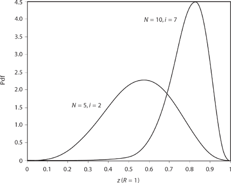
Figure 16.2. Two more nearest neighbor pdfs.

which is (as it had better be!) identical to (16.3), that is, nn₁(z) = fz(z). Figure 16.2 shows the pdf curves for i = 2 and N = 5, and i = 7 and N = 10.

16.3 What Happens When We Have Lots of Cannibals

Imagine now that N is “large,” but that we’ve allowed the island to also grow in size so that the area density of cannibals (number of cannibals per unit area) remains constant. That is, while N and R are increasing, the value of

remains fixed. (I’ll elaborate soon on just what “N is large” means.) The nearest neighbor pdf of (16.3) then becomes, with R² = N/ρπ,

or, as N → ∞ (recall Professor Grunderfunk’s challenge problem from the Preface),

Putting (16.11) into (16.1), we have for “large” N (and so of course R → ∞ that

From integral tables we have

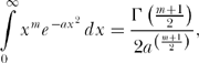
where Γ is the gamma function. For our problem m = 2 and a =,ρπ and so for “large” N with a given density of cannibals (ρ), we get the amazingly simple result

where I’ve used both the gamma function’s recursive property of Γ(x + 1) = x Γ(x) and the particular value³ .

To see what N “large” means, let’s just substitute (16.10) into (16.12) without worrying about the size of N. That is, let’s write

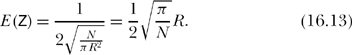
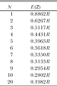
If we now compute E (Z) from (16.13) then we can see how large N has to be to give values close to the correct values given in our first table calculated from (16.6).

By the time we get to N = 10, E (Z) from (16.13) is less than 4% different from the exact value of E(Z) from (16.6); that is, N doesn’t really have to be very big at all to be “large.”

16.4 Serious Physics

We can extend our cannibal problem to one of far more physical interest¹ if we move off our two-dimensional island surface and into three-dimensional space. Suppose now that we have N stars (considered as point objects) scattered uniformly throughout a spherical region of space with radius R. At the center of this region sits the N + 1th star. Our question now is, what is the expected distance from the center star to its nearest neighbor star? The analysis goes through pretty much as it did with the cannibal problem—and that, of course, is why I did the cannibal analysis in the first place!

Let fz(z) be the pdf of the random variable Z, which represents the distance between the center star and its nearest neighbor. We next imagine a sphere of radius z centered on the center star. The probability that any individual one of the N neighbor stars surrounding the center star is inside that sphere, that is, is within distance z of the center star, is

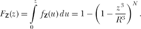
The distribution function of Z is F_z(z)=P(Z≤z) = where P (Z > z) is the probability all N neighbor stars are more than distance z from the center star. Since the probability any individual one of the N neighbor stars is more than distance z from the center star is then is the probability all N neighbor stars are more than distance z from the center star, and so P(Z > z) = and therefore

At this point you should be able to complete the analysis and thus answer the following challenge problem question:

CP. P16.1:

Find an expression for E(Z) for our star problem, and numerically evaluate E(Z) for N = 1 to 10. Also, try your hand at:

CP. P16.2:

What is the probability that the most distant star from the center star is no closer than 0.9R, as a function of N? Note that this probability should increase and approach one as N increases; does your expression have that behavior? How big does N have to be for this probability to be greater than 0.99?

Notes and References

1. See note 6 in Discussion 14.

2. For a complete discussion of this procedure for generating the radial distances of points uniformly distributed over a circle, see my book, Digital Dice (Princeton, N.J.: Princeton University Press, 2008, pp. 16-18). This procedure gives us only the radial distance of the points from the origin, of course, and says nothing about the angular dispersion of the points. But that’s okay, because we don’t need the angular information for H’s problem. H doesn’t care about what direction it is to his nearest neighbor, only how far he has to travel.

3. See note 4 in Discussion 7 for the definition of the gamma function, and my book, An Imaginary Tale: The Story of (Princeton, N.J.: Princeton University Press, 2007, pp. 175-176, for both the recursive property of Γ(x) and the calculation of the function’s value at x = 1/2).

4. This entire mathematical discussion (except for the cannibals) was motivated by reading the physics papers by A. M. Stoneham, “Distributions of Random Fields in Solids: Contribution of the Nearest Defect” (Journal of Physics C, January 20, 1983, pp. 285-293), and M. Berberan Santos, “On the Distribution of the Nearest Neighbor” (American Journal of Physics, December 1986, pp. 1139-1141, and October 1987, p. 952).