
 The Big Noise
Every sound shall end in silence, but the silence never dies.
—Samuel Miller Hageman, “Silence” (1876)
18.1 An Interesting Textbook Problem
During the autumn quarter of my sophomore year (1959–1960) at Stanford I took Math 130, my first course in differential equations. The assigned textbook was Ralph Palmer Agnew’s classic Differential Equations. I have kept my copy of Agnew all these past fifty years since, and as I write it is open on my desk in front of me to page 40. On that page is a problem I’ve always remembered because it described such a novel idea (to me) that I was immediately and forever fascinated by it. This will be our final discussion of the book (final serious physics discussion, that is—but don’t overlook the “for fun” bonus discussion at the very end of the book!), and I think Agnew’s problem presents just the right note for serving in that exit role. The book will end—metaphorically anyway—with a “big bang.” Here’s what Professor Agnew wrote:
The pilot of a supersonic jet airplane wishes to make a big noise at point O by flying around O in a path such that all of the noise he makes is heard simultaneously at O. His Mach number is M [named after the famous German physicist Ernst Mach (1838–1916), whose philosophical writings greatly influenced Albert Einstein], which means his speed is Mc where c is the speed of sound, and M > 1 because the speed [of the jet airplane] is supersonic. Letting O be the origin of a plane with polar coordinates θ and r, and supposing that the pilot starts at time t = 0 from the point θ = 0, r = a, and flies around O in the positive direction [that is, counterclockwise for an observer looking downward], find the simplest equation of the path.
There then followed a very brief sketch by Agnew for how to set up the analysis mathematically. I thought the whole idea of “the big noise” to be a hugely entertaining one. And why wouldn’t I? I was, after all, a college sophomore!
So, I was greatly interested when, some years later, I came across a paper1 in the American Journal of Physics that solved the problem all over again (no citation of Agnew’s or any other textbook, for that matter, was given). Then, a bit later, yet another paper2 appeared in the same journal to give what the author said was “perhaps a somewhat simpler derivation of the trajectory.” The major contribution of that paper was not in the mathematics, however, but rather in its novel illustration of the physics of the problem. Instead of a jet airplane flying faster than the speed of sound, the “noise disturbance” was produced by the detonation of one end of a narrow strip of high explosive, with the detonation point then swiftly (7,300 meters/second) propagating along the strip. The strip was bent into the shape of the path that would have the shock front of the detonation, generated at every point along the strip, arrive at point O at the same time. The paper included a sequence of fascinating, high-speed camera pictures demonstrating the reality of the simultaneously converging shock fronts. That is, what that second paper described is a shaped charge explosive lens that generated a tremendous impulsive force at O, a force produced by focusing the shock waves generated by a traveling explosion occurring over an interval of time. The mathematics of that lens—that is, the curve of the explosive strip—is almost as fascinating as the explosion. I’ll continue on from here with Agnew’s airplane version, but the explosion math is the same.
18.2 The Polar Equations of the Big-Noise Flight
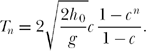
There are two general initial observations we can make about this problem without doing much mathematics. First, the entire flight, from start to the big noise finish, is of finite duration, equal to the time it takes the initial shock wave (generated at time t = 0 at point A in Figure 18.1) to reach O. If we denote that entire flying time by T, then
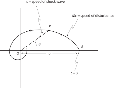
Figure 18.1. A moving disturbance an airplane traveling at speed Mc on and its shockwave traveling at speed c.
![]()
Second, the airplane itself arrives at O at time t = T, along with all of the shock waves it has generated at each instant of time over the interval 0 ≤ t ≤ T (this includes the one just generated at time T). At each such instant the shock wave starts at the airplane’s location, leaves the airplane, and then moves inward toward O at speed c. For all the shock waves and the airplane to arrive at O simultaneously, the airplane must be moving radially inward at speed c as well. Since we’ll be working in polar coordinates (r,θ) as shown in Figure 18.1, we can then write
![]()
and, since r(0) = a, we have
![]()
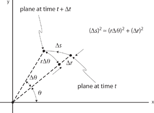
Figure 18.2. The arc-length Δs in polar coordinates.
Okay, that’s the easy stuff. Now we are ready to do some serious mathematics.
The path of the airplane, assumed to take place entirely in a plane surface, is shown in Figure 18.1 as some sort of inward spiral. Suppose P is an arbitrary point on that spiral path at time t (P = A at t = 0). Let’s write tAP as the time for the airplane to travel from A to P, and tPO as the time for the shock wave produced at P to travel from P to O. Our problem, then, is that of determining what the airplane’s path is so that
![]()
is a constant, the same for all points P on the spiral path. As I said before, it will be convenient to work in polar coordinates, and so we’ll write the coordinates of P as (r,θ), where θ is as shown in Figure 18.1 and r is the length of OP. We have, then,
![]()
To determine the arc-length of AP, take a look at Figure 18.2. There you’ll see the airplane at time t at (r + Δr,θ), moving to (r,θ + Δθ) at time t + Δt, along the airplane’s inward spiral path through the “small” arc-length Δs. If all the delta quantities are “small,” then the Pythagorean theorem tells us that
![]()
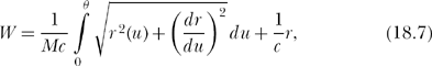
and, in the limit as the delta quantities go to zero and become differentials, we can write
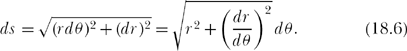
Since arc-length is ∫ ds, then using (18.2) we can write (18.5) as
where of course r = r(θ), and the u in (18.6) is simply a dummy variable of integration.
Now, here’s the crucial observation: by definition, W is a constant. Thus, W is independent of P (that is, of θ). So, it must be that
![]()
Differentiating the right-hand side of (18.6) with respect to θ (take a look back at CP 5.1 for how to differentiate an integral), and setting the result equal to zero, we arrive at
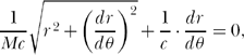
or, with just a bit of algebra and separating variables, we have
![]()
This last result is easy to integrate:
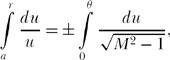
or
![]()
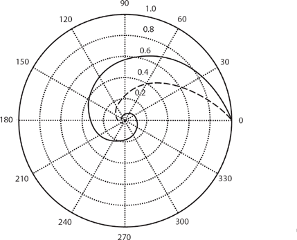
Figure 18.3. Two big noise flight paths.
or, finally,
![]()
where I’ve used the minus sign in the exponent because we know, physically, that limθ→∞r(θ) = 0. Figure 18.3 shows the “big noise” flight path (normalized polar plots of r/a) for M = 3 (solid line) and M = 1.5 (dotted line).
As Agnew writes of (18.8),
This path is a spiral. It is easy to imagine that a pilot could follow this spiral as long as r is sufficiently great. It is not so clear that the pilot and airplane could accomplish and survive the operation of making an infinite set of turns around [O to reach O] when t = a/c.
What does Agnew mean by this? He doesn’t say, leaving it to his readers to explore the problem on their own, but I think it clear that he was thinking of the ever increasing acceleration experienced by the pilot and the airplane as they spiral inward to, and spin ever more rapidly around, O. To calculate this acceleration we will need to know both r and θ as functions of time, not just r as a function of θ as given by (18.8). We already know r(t), from (18.3), so let’s now find θ(t).
Combining (18.3) and (18.8), we have
![]()
or
![]()
Using (18.2),
![]()
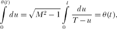
or, using (18.1),
![]()
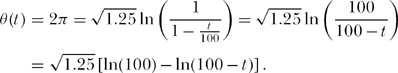
where T is the (finite) duration of the big-noise flight. It is easy to integrate (18.10), with the initial condition of θ(0) = 0:
or, with the change of variable v = T − u (and so dv = −du),
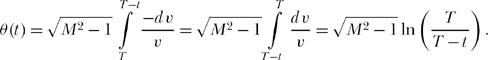
That is,
![]()
Notice that if M = 1 (the airplane is not really supersonic) then θ(t) = 0 for all t, that is, the airplane does not fly a spiral path around O but rather always moves straight in along the horizontal axis directly toward O. You can also see now, too, that even though the total flight time is finite for M > 1, the number of loops around O is infinite because limt→(T)θ(t) = ∞ (this explains Agnew’s “infinite set of turns” phrase). Now, with (18.3) and (18.11) in hand, we are ready to calculate the acceleration of the pilot and airplane as they fly a big-noise path.
18.3 The Acceleration on a Big-Noise Flight Path
To calculate the acceleration of a moving point in polar coordinates, in general, I’ll take advantage of the vector nature of the complex exponential eiθ(t) where ![]() . The famous expansion formula of Euler says
. The famous expansion formula of Euler says
![]()
and the right-hand side of this expression is a vector of unit length making angle θ(t) at time t with the x-axis, directed outward from the origin. Since our moving point isn’t always unit distance from the origin of our coordinate system (O in the big noise problem), we write the so-called position vector of the moving point as
![]()
I’m using bold notation for p(t) to indicate it is a vector. Notice carefully that r(t) is not a vector; it is the length of the vector ![]() . It is the
. It is the ![]() all by itself that provides the vector nature to p(t).
all by itself that provides the vector nature to p(t).
From (18.12) we can find the moving point’s velocity and acceleration vectors, v(t)and a(t), respectively, by successive differentiations. For example, for v(t) we have
![]()
or, more transparently,
![]()
The first term on the right-hand side of (18.13) is a vector with length ![]() that is pointing in the same direction as
that is pointing in the same direction as ![]() if
if ![]() and in the direction opposite that of
and in the direction opposite that of ![]() if
if ![]() (that is, radially inward). The second term on the right in (18.13) is a vector, too, but now we must remember that the vector nature of that term is due to
(that is, radially inward). The second term on the right in (18.13) is a vector, too, but now we must remember that the vector nature of that term is due to ![]() , not just
, not just ![]() . The presence of the factor i produces a unit vector that is rotated3 90 degrees counterclockwise from
. The presence of the factor i produces a unit vector that is rotated3 90 degrees counterclockwise from ![]() . So, the second term of (18.13) is a vector with length
. So, the second term of (18.13) is a vector with length ![]() that is pointing 90 degrees counterclockwise from
that is pointing 90 degrees counterclockwise from ![]() if
if ![]() and 90 degrees clockwise from
and 90 degrees clockwise from ![]() if
if ![]() .
.
The first term of (18.13) is the radial velocity and the second term is the tangential velocity. The magnitude of their vector sum is the speed (a scalar) of the moving point, and it is instructive to calculate it for the big-noise problem. That is, the speed of the jet airplane is, using (18.1), (18.2), (18.3), and (18.10),
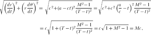
a constant for all t which is, of course, correct (take a look again at Agnew’s original presentation of the big-noise problem).
To find the acceleration of the moving point, we differentiate (18.13) and get
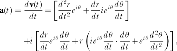
or, collecting terms,
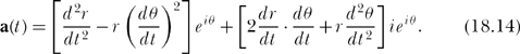
Again, we can calculate the magnitude of the acceleration—which is physically what most interests the pilot—from the component radial and tangential accelerations in (18.14). Thus,
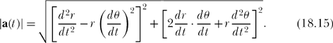
Since (18.3) tell us that ![]() for the big-noise problem, and using our earlier result of (18.10) to calculate
for the big-noise problem, and using our earlier result of (18.10) to calculate ![]() as
as
![]()
we can use these and our earlier results for all the other terms in (18.15) to write
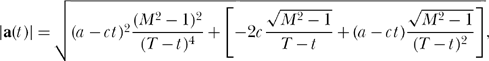
which, after just a bit of routine algebra, becomes the remarkably simple
![]()
Suppose, as an example of what (18.16) can tell us, that the pilot starts his big noise flight at a distance of a = 100,000 feet from O, flying at one-and-a-half times the speed of sound (M = 1.5). As a fairly good approximation to the speed of sound, I’ll use c = 1,000 feet/second, which means the entire flight time is T = 100 seconds. The big question, of course, is, can the pilot actually survive this flight? From (18.16) we see that the acceleration experienced by the pilot is
![]()
A military combat pilot can probably remain aware of his surroundings up to about seven gravities of acceleration (7 gees). Beyond that value blood flow to the brain is reduced below that necessary for a human to remain conscious, much less functional. This acceleration will be reached when
![]()
or, solving for t, when t = 92.6 seconds. That looks like almost all of the flight—but looks are deceiving! From (18.3) the plane will, at that time, then be 7,400 feet from O and will have looped around O through an angle, from (18.11), of
![]()
This is an angle of just 167 degrees, less than one-half a single loop around O. There are still an infinity of loops to go in the remaining 7.4 seconds of flight time. That is, when the flight is more than 92% finished in time, it has only just begun in terms of looping around O. If this was a Disney World ride, I think I’d take a pass.
CP. P18.1:
At what time does the pilot in the above analysis complete the first loop around O, and what is his acceleration at that moment? Assume both the plane and the pilot are indestructible.
Notes and References
SOLUTIONS TO THE CHALLENGE PROBLEMS
Challenge Problem P.1
The hyperbolic functions are defined as follows:
![]()
So,
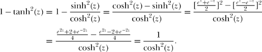
Thus,
![]()
and so the right-hand side of our “great truth” is
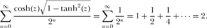
Now, on the left-hand side of the “great truth” you should recognize that ![]() , and also that sin2(y) + cos2(y) = 1. Thus, the left-hand side is simply
, and also that sin2(y) + cos2(y) = 1. Thus, the left-hand side is simply
![]()
That is, our great truth is the undeniably true
![]()
Challenge Problem P.2
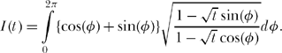
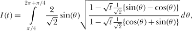
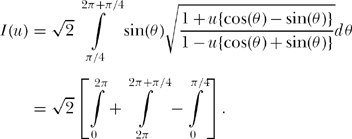
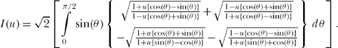
Notice that the radical in the integrand is real for all t in the interval 0 to 1, as for all φ both the numerator and the denominator are non-negative. Thus, I(t) is purely real. Now, change variable to θ = φ + π/4. Then dθ = dφ and we have
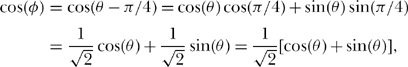
and
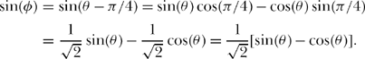
So,
or, writing ![]() ,
,
By the periodicity of the sine and cosine functions, the integrand value over the second integration interval is, for every value of θ, identical to the integrand value over the third integration interval. That is, the last two integrals cancel. Thus,
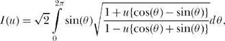
where u varies from 0 to ![]() as t varies from 0 to 1. Now,
as t varies from 0 to 1. Now, ![]() . Since cos(θ) is symmetrical around π, while sin(θ) is antisymmetrical around π, we can write the π to 2π integral as an integral from 0 to π if we replace every cos(θ) with cos(θ) and every sin(θ) with −sin(θ). That is,
. Since cos(θ) is symmetrical around π, while sin(θ) is antisymmetrical around π, we can write the π to 2π integral as an integral from 0 to π if we replace every cos(θ) with cos(θ) and every sin(θ) with −sin(θ). That is,
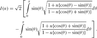
Or
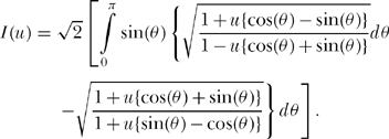
Now, ![]() . Since sin(θ) is symmetrical around π/2, while cos(θ) is antisymmetrical around π/2, we can write the π/2 to π integral as an integral from 0 to π/2 if we replace every sin(θ) with sin(θ) and every cos(θ) with −cos(θ). That is,
. Since sin(θ) is symmetrical around π/2, while cos(θ) is antisymmetrical around π/2, we can write the π/2 to π integral as an integral from 0 to π/2 if we replace every sin(θ) with sin(θ) and every cos(θ) with −cos(θ). That is,
This may look like we are taking our original tough-looking integral and making it look even more awful, but that’s an illusion. Here’s why.
If we call the first radical x, then you’ll notice that the second radical is the reciprocal of the first one and so is 1/x. Also, if we call the fourth radical y, then the third one is its reciprocal and so is 1/y. What I’ll do next is show that, over the entire interval of integration, the integrand is non-negative (and it is obviously not identically zero), so I(u) > 0, that is I(t) > 0. (The factor of sin(θ) in front of all the radicals is never negative over the integration interval, so we can ignore it.) That is, I will show you that
![]()
that is, that
![]()
that is, that
![]()
that is, that
![]()
that is, that
![]()
Now, if x ≥ y, then that last inequality says it must be true that xy ≥ 1. If we can show that both of these conclusions are actually so, then our starting inequality (that is, ![]() ) will in fact be true, and we’ll be done. So, first, is x ≥ y? The answer is yes, because that inequality is simply the assertion that
) will in fact be true, and we’ll be done. So, first, is x ≥ y? The answer is yes, because that inequality is simply the assertion that
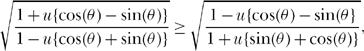
which is the assertion that
![]()
which is the assertion that
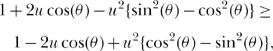
which is the assertion that
![]()
which is obviously true for all θ in the integration interval 0 to π/2 (remember, u itself is non-negative). Second, is xy ≥ 1? The answer is again yes, because that inequality is simply the assertion that
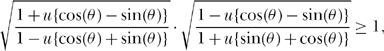
which is the assertion that
![]()
which is the assertion that
![]()
which is obviously true for all θ in the integration interval 0 to π/2 because, in that interval both cos(θ) and sin(θ) are never negative (the sum of two non-negative numbers is always at least as large as their difference). This completes the high school algebra and trigonometry proof that I(t) > 0 for all t in the interval 0 to 1. My discussion here is based on the paper by John D. Morgan III, “The Positivity of an Integral Connected with the Helium Atom Problem” (American Journal of Physics, February 1978, pp. 180–181). I have expanded on numerous points in Morgan’s paper that, for purposes of journal publication brevity, Morgan had to skip over with little mention.
Challenge Problem P.1.1
From (1.8) we have the speed of the wall end of the pole as
![]()
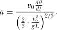
Therefore, the acceleration is, in general, before breakaway
![]()
From (1.14) we have the breakaway angle θ = θc as
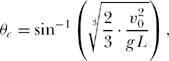
and so
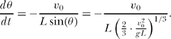
![]()
and
![]()
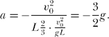
This says, at breakaway, the acceleration is
From (1.11) we have, at breakaway,
So, at breakaway, the acceleration of the wall end of the pole is
Challenge Problem P.2.1
Let D and T be the total bounce distance and time, respectively. Then, 
where
![]()
![]()
For my garage experiment, c = 0.913 and h0 = 36 inches and so D = 397 inches. We also showed that the total time from the first impact until the n-th impact is
So, as n → ∞, this becomes (because c < 1) ![]() . We have to add to this the initial drop time
. We have to add to this the initial drop time ![]() to get
to get
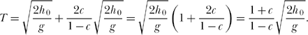
For my garage experiment T = 9.5 seconds.
Challenge Problem P.3.1
If you look back at Figure 3.10, you can see that if we remove the first two resistors, we are left with the original infinite network flipped over. Since that network is in parallel with the removed resistor “on a slant”, we can immediately write
![]()
which is just (3.1) again with R1 = R2 = 1. So, ![]() . So, even though the network of Figure 3.10 “looks different” from that of Figure 3.1, the defining equation for the input resistance is the same for both.
. So, even though the network of Figure 3.10 “looks different” from that of Figure 3.1, the defining equation for the input resistance is the same for both.
Challenge Problem P.3.2
We start with ![]() . Let u = z’ − z (and so du = dz’).
. Let u = z’ − z (and so du = dz’).
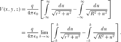
From integral tables we have ![]() , and so
, and so
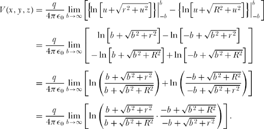
Now, ![]() and so
and so ![]() . Now, as b → ∞ the first factor inside the log function goes to 1, and the second factor goes to R2/r2. So,
. Now, as b → ∞ the first factor inside the log function goes to 1, and the second factor goes to R2/r2. So, ![]() or, at last, we have the finite
or, at last, we have the finite ![]() . There is no z dependency because the electrically charged wire is infinitely long in the z direction, and there is nothing to physically distinguish one value of z from any other.
. There is no z dependency because the electrically charged wire is infinitely long in the z direction, and there is nothing to physically distinguish one value of z from any other.
Challenge Problem P.3.3
Figure S3.11 shows an arbitrary node along the ladder, with node voltage v(n). Kirchhoff’s node current law says the current into the node equals the current out of the node. So,
![]()
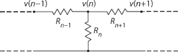
Figure S3.11. An arbitrary node of an infinite ladder.
If we multiply each resistance in this expression by the same factor k, we will still have a valid statement of Kirchhoff’s law with the same node voltages. All that changes are the individual resistor currents, which will be the original currents divided by k. In particular, the input current to the first section of the ladder will be divided by the factor k, and so we will have the original input voltage but an altered (by the factor k) input current. Thus, the input resistance changes (is divided) by the factor k.
Challenge Problem P.3.4
I don’t know the answer to this question. If I calculate the sequence of input resistances Rn to finite-length versions of the infinite ladder of Figure 3.9c (that is, ladders with n = 1, 2, 3, and 4 stages) I get R1 = 2, R2 = 1.9099, R3 = 1.9019, and R4 = 1.9090909. From this flimsy “evidence” one might conjecture that the exact result is ![]() ohms. But I can’t prove that—it may well be wrong. Any help from readers will be greatly appreciated, and a reader derivation of Rc will receive prominent display and attribution in the future paperback edition of this book.
ohms. But I can’t prove that—it may well be wrong. Any help from readers will be greatly appreciated, and a reader derivation of Rc will receive prominent display and attribution in the future paperback edition of this book.
Challenge Problem P.3.5
See the solution to Challenge Problem P.17.3.
Challenge Problem P.4.1
When the rocket motor cuts off at t = t1, let’s write the rocket’s height as h1 and its (maximum) speed at that instant as v1. From there it continues to rise upward to its maximum height (H)—let’s say the time to go from h1 to H is Δt—and then from H it falls back down to h1 in the same time interval Δt. As it falls through height h1 it is again moving at speed v1. From h1, on down to the ground the rocket’s speed obviously continues to increase beyond v1. On the upward portion of its flight, however, from zero height to h1, the rocket’s speed was always no more than v1. So, it takes longer for the rocket to accelerate from zero to v1 (from the ground to h1) than to fall from height h1 to the ground. Thus, tup > tdown.
Challenge Problem P.4.2
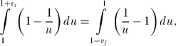
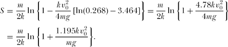
Inserting f(v) = kv into (4.4) and taking the unit speed as the terminal speed, we have

Letting u = 1 + v (and so du = dv) in the left-hand-side integral, and u = 1 — v (and so du = −dv) in the right-hand-side integral, we have
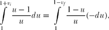
or
or
![]()
![]()
or
![]()
From (4.3)
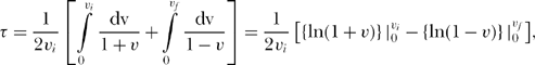
or, using the above boxed result,
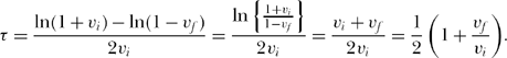
Since vf < vi for any physically plausible drag force law (including our linear one), then τ < 1 for f(v) = kv.
Challenge Problem P.5.1
Starting with
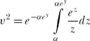
we have, from how to differentiate a product and remembering that α is a constant,
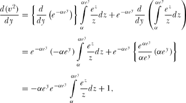
![]()
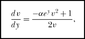
At the start of the fall v = 0, and so
![]()
Since the initial rate of change of v2 is positive, v will increase as the fall continues (as will ey—remember that y = 0 at the start of the fall and is measured in the downward direction and so increases as the fall progresses) until ![]() ; this will obviously occur after a finite fall distance. The value of v at that instant is v = V. From this point on the speed must do one of three things: (1) continue to increase beyond V, (2) remain fixed at V, or (3) start to decrease from V. Possibility (1) can be rejected because
; this will obviously occur after a finite fall distance. The value of v at that instant is v = V. From this point on the speed must do one of three things: (1) continue to increase beyond V, (2) remain fixed at V, or (3) start to decrease from V. Possibility (1) can be rejected because
![]()
which says
and, since both v and ey are increasing, the boxed expression says ![]() because the first term in the numerator of the right-hand side of the boxed expression is growing ever more negative during the fall. But if v is to be increasing beyond V, we must have
because the first term in the numerator of the right-hand side of the boxed expression is growing ever more negative during the fall. But if v is to be increasing beyond V, we must have ![]() , and we have a contradiction. Possibility (2) can also be rejected, because that says
, and we have a contradiction. Possibility (2) can also be rejected, because that says ![]() while ey continues to increase, and so the first term in the numerator of the right-hand side of the boxed expression is growing ever more negative during the fall and so, again, that says
while ey continues to increase, and so the first term in the numerator of the right-hand side of the boxed expression is growing ever more negative during the fall and so, again, that says ![]() , and we have a contradiction. Therefore, what actually happens must be our final possibility, possibility (3), that is, v decreases from V. That says
, and we have a contradiction. Therefore, what actually happens must be our final possibility, possibility (3), that is, v decreases from V. That says ![]() , which is not in an inescapable contradiction with the boxed expression, just so long as the increase in ey more than compensates for the decrease in v. Thus, v increases from 0 to V (which is, in fact, the maximum speed Vmax) and thereafter decreases, just as shown in the curves of Figure 5.3.
, which is not in an inescapable contradiction with the boxed expression, just so long as the increase in ey more than compensates for the decrease in v. Thus, v increases from 0 to V (which is, in fact, the maximum speed Vmax) and thereafter decreases, just as shown in the curves of Figure 5.3.
Challenge Problem P.6.1
From (6.7) we have x(t) = recos(αt), ![]() . Thus, the anvil’s speed is
. Thus, the anvil’s speed is ![]() . When the anvil arrives in Hell, located at x = 0 (which means
. When the anvil arrives in Hell, located at x = 0 (which means ![]() ), its speed is
), its speed is ![]() . A massm on the surface of Earth has weight mg, where
. A massm on the surface of Earth has weight mg, where ![]() and so
and so ![]() . So,
. So, ![]() which gives the anvil’s arrival speed as
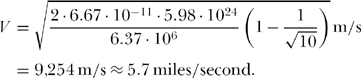
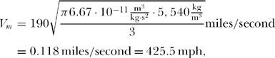
which gives the anvil’s arrival speed as ![]() . Plugging in numbers, the anvil arrives in Hell with speed
. Plugging in numbers, the anvil arrives in Hell with speed ![]() feet/second = 25,947 feet/second, which is ≈4.9 miles/second. This may be slower or faster than the speed of the proverbial “bat out of Hell,” a calculation that remains out of the realm, at least for the time being, of mathematical physics
as we know it.
feet/second = 25,947 feet/second, which is ≈4.9 miles/second. This may be slower or faster than the speed of the proverbial “bat out of Hell,” a calculation that remains out of the realm, at least for the time being, of mathematical physics
as we know it.
Challenge Problem P.7.1
To calculate ![]() begin by defining D as
begin by defining D as ![]() . Then, changing variables to u = x2 (and so du = 2x dx) and v = y2 (and so dv = 2y dy), we have
. Then, changing variables to u = x2 (and so du = 2x dx) and v = y2 (and so dv = 2y dy), we have ![]() , that is,
, that is, ![]() because u, v, x, and y are all, of course, dummy variables of integration. Next, define S as
because u, v, x, and y are all, of course, dummy variables of integration. Next, define S as ![]() Then, adding the two boxed expressions,
Then, adding the two boxed expressions, ![]() and so, rearranging and dividing by 2,
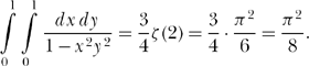
and so, rearranging and dividing by 2, ![]() . Now, as shown in the discussion the last integral on the far right is ζ(2), and so the answer to our first question is
. Now, as shown in the discussion the last integral on the far right is ζ(2), and so the answer to our first question is
To calculate ![]() notice that the second boxed expression says
notice that the second boxed expression says 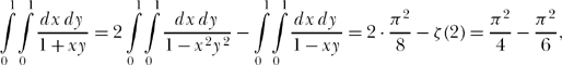 , and so
 ![]()
Challenge Problem P.7.2
If you calculate the Fourier series expansion of f(x) = x3 over the interval −π to π, you should get
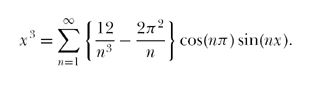
If, for example, you set x = 1, then the left-hand side of the expression in the box is of course 1, while a numerical evaluation of the sum on the right-hand side, using the first one million terms, is 0.99999840332. … Notice, however, that if we set x = π, the summation is not π3 but rather zero because of the sin(nx) factor−sin(nπ) = 0 for all integer n. This behavior is caused by the fact that a Fourier series expansion of a discontinuous function converges, at a discontinuity, to the average of the function values on each side of the discontinuity (and the average of +π3 and −π3 is, of course, zero). If it isn’t clear why f(x) = x3 is discontinuous at x = π, then you should sketch x3 over the interval −π to π, and then make the periodic extension of that fundamental period to cover the entire x-axis. In fact, there is no value to which we can set x in the boxed expression that gives anything on the right-hand side of use, that is, anything that has ζ (3) in it.
Challenge Problem P.8.1
From (8.15), ![]() which is easily expanded to give
which is easily expanded to give ![]() This is quadratic in v02 and so
This is quadratic in v02 and so ![]() or, as Rm >> h,
or, as Rm >> h, ![]() is the horizontal speed of the shell. Now, for point-blank fire, the time of flight T is the time for the shell to fall vertically to the ground through a distance of h, that is,
is the horizontal speed of the shell. Now, for point-blank fire, the time of flight T is the time for the shell to fall vertically to the ground through a distance of h, that is, ![]() , or
, or ![]() So,
So, ![]() or, at last,
or, at last, ![]() For Rm = 20,000 feet and h = 4 feet,
For Rm = 20,000 feet and h = 4 feet, ![]() feet, which is surprisingly (I think) small. For the obvious purpose of point-blank fire, however, it is big enough.
feet, which is surprisingly (I think) small. For the obvious purpose of point-blank fire, however, it is big enough.
Challenge Problem P.9.1
From (9.19) we have
Now, as → we have
![]()
which is in very good agreement with the computer value of 399.1 feet. (If you use more than three decimal places in the intermediate calculations—which is all I used on my hand calculator—as well as 146.667 ft/s for the initial speed of 100 mph instead of 146.7 ft/s, then the agreement is even better.)
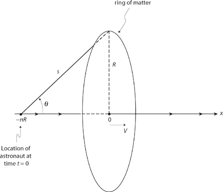
Figure S10.4. The geometry of the ring accelerator.
Challenge Problem P.10.1
Let the mass of the astronaunt be m and his speed be v. Then, from the geometry of the problem shown in Figure S10.4, we can write the gravitational force “felt” by the astronaunt that accelerates him along the x-axis toward the ring’s center as ![]() where
where ![]() and
and ![]() Thus,
Thus, ![]()
Since ![]() and
and ![]() then
then ![]() and so v
and so v ![]() Integrating indefinitely, with C the constant of integration,
Integrating indefinitely, with C the constant of integration, ![]() Next, change variable to u = x2 + R2 (and so
Next, change variable to u = x2 + R2 (and so ![]() ). Then
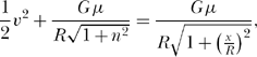
). Then ![]() Since the astronaut starts from rest (V = 0) at x = −nR, we have
Since the astronaut starts from rest (V = 0) at x = −nR, we have
![]()
or
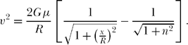
We know v = V at the ring’s center (x = 0), and so
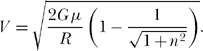
If, for example, the ring has the mass and radius of the Earth, and (to pick a value at random) if n = 3, then
The maximum possible value for V is attained when n is very large, and is 11,190 m/s ≈ 6.9 miles/second. If n = 0 (that is, if the astronaut starts at rest at the ring’s center), then our expression for V reduces to the obviously correct V = 0. To check the two claims made for Niven’s ring, first recall that the acceleration at the ring’s inner surface is, in feet/second2 (where v is the ring rotation speed and r is the ring’s radius), given by
![]()
which is just slightly more than 1 g (32.2 ft/s2), and that the area of the ring’s inner surface (in units of the Earth’s surface area) is (where w is the ring’s width and R is the Earth’s radius) given by
![]()
which is pretty nearly the claimed factor of three million.
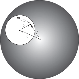
Figure S10.5. Calculating the gravity inside a spherical cavity.
Challenge Problem P.10.2
Figure S10.5 shows the geometry of the spherical Earth with a spherical cavity. A mass m is arbitrarily positioned inside the cavity. The vector from the center of the Earth to the center of the cavity is a, the vector from the center of the cavity to m is b, and the vector from the the center of the Earth to m is c. By the very definition of vector addition, we have c = a + b. Now, imagine first that there is no cavity. Then, the gravity force on m due to a solid Earth is, from the second superb theorem, due only to that part of the Earth no farther from the center of the Earth than ∣c∣= c, and that force is directed toward the center of the Earth (along c)(c is, of course, the length of c). This force is therefore the vector ![]() where
where ![]() is the unit vector pointing along c toward the center of the Earth, that is, in the direction opposite that of c. Simplifying, this force is
is the unit vector pointing along c toward the center of the Earth, that is, in the direction opposite that of c. Simplifying, this force is ![]() c. Next, to account for the cavity, we “create” it by inserting into the Earth a sphere with negative density -ρ The gravity force on m due to just this negative mass sphere is, again, because of the second superb theorem, due only to that mass no farther from the cavity’s center than ∣b∣ = b, where b is the length of b. But now, of course, that force is a repulsive force, directed away from the cavity’s center along the direction of b. This force is the vector
c. Next, to account for the cavity, we “create” it by inserting into the Earth a sphere with negative density -ρ The gravity force on m due to just this negative mass sphere is, again, because of the second superb theorem, due only to that mass no farther from the cavity’s center than ∣b∣ = b, where b is the length of b. But now, of course, that force is a repulsive force, directed away from the cavity’s center along the direction of b. This force is the vector ![]() b.
b.
The total gravity force on m is the sum of the two individual forces, which is ![]() . But since c = a + b then b − c = −a, and so the total gravity force on m is just
. But since c = a + b then b − c = −a, and so the total gravity force on m is just ![]() where
where ![]() is the unit vector from the center of the cavity to the center of the Earth. This is a force with constant magnitude
is the unit vector from the center of the cavity to the center of the Earth. This is a force with constant magnitude ![]() , independent of the location of m within the cavity. There is no dependency on either the radius of the Earth or the radius of the cavity (I don’t think this is at all obvious before doing the analysis). The magnitude of the force depends only on m, on the density of the Earth, and on how far apart the centers of the Earth and on the cavity are. The direction of the force is everywhere in the cavity parallel to the line joining the two centers, and directed to the Earth’s interior (but not toward the center of the Earth except in the special case where m is at the center of the cavity).
, independent of the location of m within the cavity. There is no dependency on either the radius of the Earth or the radius of the cavity (I don’t think this is at all obvious before doing the analysis). The magnitude of the force depends only on m, on the density of the Earth, and on how far apart the centers of the Earth and on the cavity are. The direction of the force is everywhere in the cavity parallel to the line joining the two centers, and directed to the Earth’s interior (but not toward the center of the Earth except in the special case where m is at the center of the cavity).
Challenge Problem P.11.1
Let r, Ts, and Tm be the distance of the satellite from the Earth’s center, the period of the satellite, and the period of the Moon, respectively. Then, from Kepler’s third law, and using the given distance of the Moon from the Earth’s center as 38, 850 miles, we have
![]()
Since the satellite is geostationary we have Ts = 1 day, and since Tm = 27.3 days, then we can solve for r as
![]()
The satellite is therefore 26,344 — 3,960 = 22,384 miles above the surface of Earth.
Challenge Problem P.12.1
We can solve this problem with just a bit more generality than asked for, and then get our answers as special cases. Suppose the density of a planet increases linearly from ρ0 at the surface to nρ0 at the center. (Thus, n = 2 for Planet 1 and n = 3 for Planet 2.) Then, the density is ![]() where R is the radius of the planet and r is the distance from the center. The planet mass M is
where R is the radius of the planet and r is the distance from the center. The planet mass M is
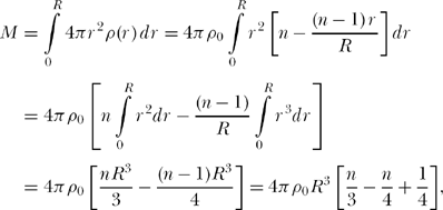
or ![]() Thus,
Thus,
Planet 1 mass (with n = 2) = ![]()
Planet 2 mass (with n = 3) = ![]()
and so the percent increase in mass from Planet 1 to Planet 2 is
![]()
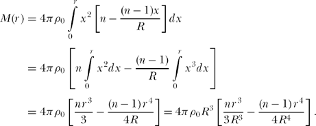
To calculate the percent increase in pressure Pc at the center of Planet 2 compared to the center pressure of Planet 1, I’ll use the differential equation of static equilibrium of (12.14): ![]() We already have ρ(r) from above, so all we need to write this differential equation is g(r). The mass of the planet within a sphere of radius r is (with x as a dummy variable of integration) given by Since the gravitational force on a mass m at distance r ≤ R from the center of the planet is
We already have ρ(r) from above, so all we need to write this differential equation is g(r). The mass of the planet within a sphere of radius r is (with x as a dummy variable of integration) given by Since the gravitational force on a mass m at distance r ≤ R from the center of the planet is ![]() , then
, then ![]() and so
and so ![]() . Thus,
. Thus,
![]()
![]()
Integrating r from 0 (where P = Pc) to r = R (where P = 0), we have
or, after some simple algebraic reduction, ![]() . So,
. So,
![]()
![]()
and therefore the percent increase in center pressure from Planet 1 to Planet 2 is
![]()
Challenge Problem P.12.2
With reference to Figure S12.7, let d denote the distance along the curved surface of the Earth between the points A and B. The angle θ between the two radii to A and B is ![]() where R is the radius of the Earth. Thus, the half-angle
where R is the radius of the Earth. Thus, the half-angle ![]() Now, with r0 as the distance from the center of the Earth to the center of the tunnel,
Now, with r0 as the distance from the center of the Earth to the center of the tunnel, ![]() or
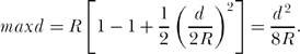
or ![]() . As the figure illustrates, the maximum depth, maxd, of the tunnel beneath the Earth’s surface is
. As the figure illustrates, the maximum depth, maxd, of the tunnel beneath the Earth’s surface is
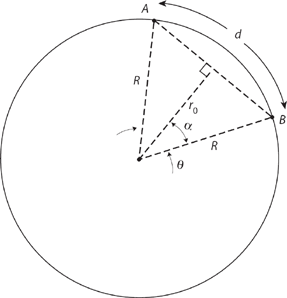
Figure S12.7. A tunnel through the Earth.
![]()
For A as New York City and B as either Boston or Philadelphia, d < < R, and since ![]() for x < < 1, then, to a good approximation,
for x < < 1, then, to a good approximation,
For the New York City-Boston tunnel, with R = 3,960 miles and d = 190 miles, which is pretty deep, but may be not impossibly deep. For the New York City-Philadelphia tunnel, with d = 85 miles,
![]()
![]()
which seems (to me) to be within the realm of the “reasonably possible”.
Challenge Problem P.12.3
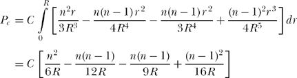
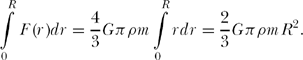
If we take the center of the Earth as our zero potential energy reference point, then a mass m on the surface of the Earth has a potential energy equal to the energy required to transport it (against the Earth’s gravity force F(r)) from the center to the surface. This force is given by
![]()
where of course M(r) is the mass inside a sphere of radius r and ρ is the (assumed constant) density of the Earth. The transport energy is then
Now, if r0 is the distance from the center of the Earth to the center of the tunnel (where the traveler’s speed is maximum = Vm), we then have, by conservation of energy,
![]()
where the left-hand side is the change in potential energy from the surface to the tunnel’s midpoint and the right-hand side is the change in the kinetic energy. So,
![]()
As shown in the previous solution, ![]() as long as d < < R. So,
as long as d < < R. So,
![]()
For the New York City-Boston tunnel,
which is far less (and far more reasonable) than is Goddard’s speed. Since the maximum speed scales linearly with d, then for the New York City-Philadelphia tunnel we get the even less extreme speed of Vm= 190 mph. For a full-diameter trip we simply set r0 = 0 and get
Compare this result with the answer to Challenge Problem P.6.1.
Challenge Problem P.12.4
Write the acceleration of gravity as g. The mass falling from point A takes time TA to fall a distance of 2R. Thus, ![]() or,
or, ![]() The mass at point B slides a distance of l. Since, as given in the hint, the triangle ABC is a right triangle, then if θ is the angle the wire (along which the sliding mass travels) makes with the horizontal, then θ is also the vertex angle of the triangle at A. Thus, l/2R = sin(θ). Now, the acceleration of the mass along the wire is a = g sin(θ) = l g/2R. If the time for the slide is TB, then
The mass at point B slides a distance of l. Since, as given in the hint, the triangle ABC is a right triangle, then if θ is the angle the wire (along which the sliding mass travels) makes with the horizontal, then θ is also the vertex angle of the triangle at A. Thus, l/2R = sin(θ). Now, the acceleration of the mass along the wire is a = g sin(θ) = l g/2R. If the time for the slide is TB, then ![]() Since l cancels on both sides, then TB2 = 4R/g. But this is TA2. So, TB = TA.
Since l cancels on both sides, then TB2 = 4R/g. But this is TA2. So, TB = TA.
Challenge Problem P.13.1
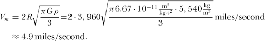
Figure 13.8 is reproduced below (as Figure S13.11a) with the subsquares labeled in bold as a, b, c, and so on. If we call the edge lengths of the a, b, and c subsquares x, y, and w, respectively, then we can immediately write the edge length of d as y − w, and the edge length of g as x − y − w, as shown. That tells us that the edge length of h is w − (x − y − w) = 2w − x + y, as shown. Then, comparing c and h with d, we see that w + 2w − x + y = y − w, that is, x = 4w. Continuing, from g and h we see that the edge length of f is (2w − x + y) − (x − y − w) = 3w − 2x + 2y, as shown. The edge length of i is the sum of the edge lengths of f, h, and d, that is, (3w − 2x + 2y) + (2w − x + y) + (y − w) = 4w − 3x + 4y, as shown. And finally, the edge length of e is obviously (x + y) − (4w − 3x + 4y) = 4x − 4w − 3y. Now, using the vertical constraints on the far left and right edges, we have (x) + (4x − 4w − 3y) = (y) + (y − w) + (4w − 3x + 4y), which reduces to 8x = 7w + 9y. Remembering that x = 4w, we have 32w = 7w + 9y, or 25w = 9y. An obvious solution of these two relations, x = 4w and 25w = 9y, is y = 25, w = 9, and x = 36. If these values are inserted into the expressions for the individual subsquare edge lengths we get the solution tiling, with no two sub-squares equal, shown in Figure S3.11b.
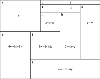
Figure S13.11a. Figure again (with symbolic edge lengths).
Challenge Problem P.13.2
Let’s label the smallest subsquare of a tiling as S, which we know from the discussion in the text is not on the border. Following the hint, let’s assume we have five subsquares surrounding S. To do this, we must have two (each larger than S, of course) sub-squares along one of S’s edges, something like as shown in Figure S13.12a. Then, adding yet another subsquare (call it X)—which must go along one of S’s vertical sides, because if X is along S’s bottom side then no (larger than S) subsquare could fit along either vertical side of S—we have Figure S13.12b. And now you can see we are only one step away from failure. If we position yet another (larger than S) subsquare along the bottom side of S then we can’t get a (larger than S) subsquare along the remaining vertical side of S, and vice versa. If we assume S has even more than five adjacent neighbors, then we obviously have a similar disaster. So, the only possible tiling is one with exactly one subsquare along each side of S (that is, four adjacent neighbors), as shown in Figure S13.12c.
Figure S3.11b. The final tiling.
Challenge Problem P.14.1
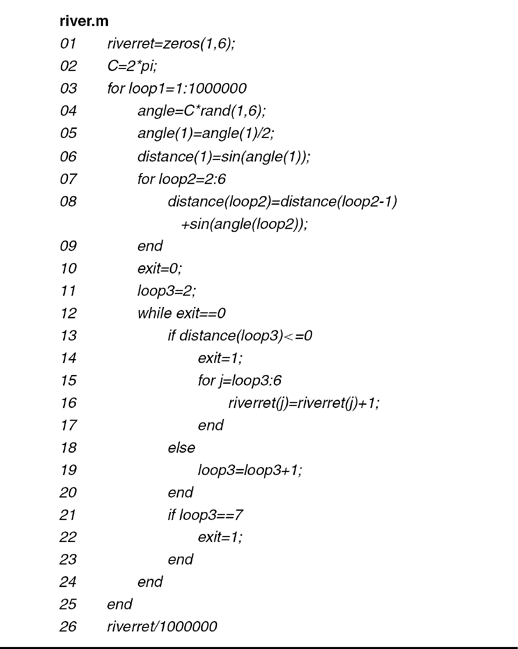
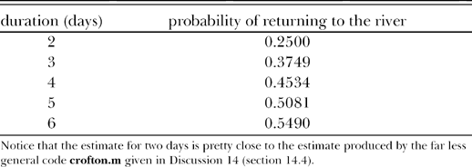
The MATLAB code river.m performs one million walks, each six days in duration. The fundamental idea behind the code is that, if a return to the river occurs on day x, then a return to the river occurs for all walks of duration x, x + 1, x + 2,…. Note carefully that a return to the river does not have to occur on the last day of a walk. Indeed, there may be multiple returns to the river during a given walk, but only the occurrence of the first return matters. In detail, then, here’s how river.m works. Line 01 creates the six-element vector riverret, initially with all its elements set to zero. When the simulation ends riverret(k) will equal the number of times a journey of duration k days returned to the river. Line 02 simply sets the constant C to 2π I did that here to avoid constantly multiplying 2 by π when the code gets down to work. The outermost loop, defined by lines 03 and 25, counts off the one million journeys. When that loop is entered, at line 04, to start each new simulated journey, the vector angle is loaded with six random numbers uniformly distributed from 0 to 2π. These are the angles, one after the other, that our traveler starts off with each new day; of course, the value of the first angle should be limited to the interval 0 to π, and that explains line 05. Line 06 generates the distance the traveler is from the river at the end of the first day, storing it as distance(1), and then lines 07 through 09 fill in the rest of the elements of the vector distance; that is, distance(k) is the distance the traveler is from the river at the end of day k. Lines 10 through 20 now look at distance to determine if a return to the river has occurred (in line 13). This examination begins with distance(2)—notice that the variable loop3 is initialized to 2 in line 11, and the variable exit is initialed to 0 in line 10—and continues until the first occurrence of a return. When (if) that happens, exit is set to 1 in line 14 (to terminate the while loop that is examining distance), and then all elements of riverret indexed on the current value of loop3 up to 6 are incremented by 1 to record a return to the river for all journeys of durations loop3 days to 6 days. If a first return does not occur for a journey of duration loop3 days, however, then line 19 increments loop3 by 1 (and lines 21 through 23 force exit=1 to terminate the while loop if the code has examined all six elements of distance). This all happens all over again for a total of one million journeys, and then line 26 prints the code’s estimates for the probability of a return to the river for journeys of length k days. When run, river.m produced the following estimates:
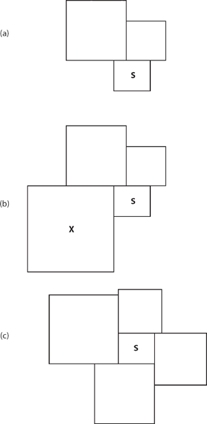
Figure S13.12. The neighbors of S.
river.m
Challenge Problem P.14.2
From (14.1) we have the pdf of the random variable X as
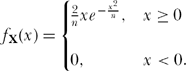
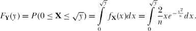
That is, X is a Rayleigh random variable. To find the pdf of Y = X2, we first find Y’s distribution function and then differentiate. So,
![]()
or, since X is never negative,
This integral is actually doable, but why bother? We are, after all, just going to differentiate the result! So, let’s differentiate the integral (using Leibnitz’s formula) straightaway to get
![]()
That is,
which is, indeed, the pdf of an exponential random variable, as was to be shown.
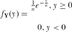
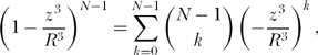
Challenge Problem P.15.1
The MATLAB code cp15.m estimates the pdf of a 21-step stretched walk with s = 1.01. The result is shown in Figure S15.6.
Challenge Problem P.16.1
Differentiating the expression given in the problem statement, ![]() or
or ![]()
then
and so
or, at last,
Evaluating numerically, we have:
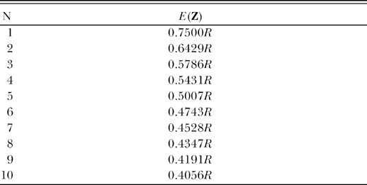
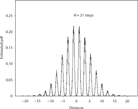
Figure S15.6. Stretched walk pdf for s = 1.01
Challenge Problem P.16.2
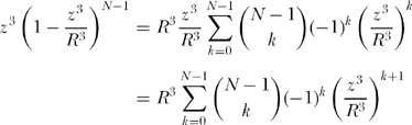
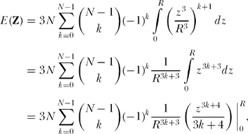
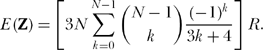
Let W be the random variable representing the distance of the most distant star from the center star; the distribution function of W is FW(w) = P(W ≤ w). Thus, since w3/R3 is the probability each of the individual neighbor stars is within distance w of the center star—and so all the neighbor stars are within distance w of the center star (all the other neighbor stars must, by definition, be even closer than the farthest star)—then
![]()
For the most distant star to be no closer than 0.9R, W must be in the interval 0.9R ≤ W ≤ R. The probability of that is
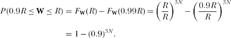
For this probability to exceed 0.99, that is, for 1 − (0.9)3N > 0.99, we have 0.01 > (0.9)3N, or, taking logs on both sides (to the base 10),
![]()
which of course means that N ≥ 15.
Challenge Problem P.17.1
If ![]() then bc + bd = ad + bd, and so bc = ad. This says that
then bc + bd = ad + bd, and so bc = ad. This says that ![]() and so
and so ![]() Thus,
Thus,
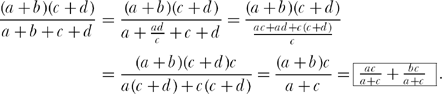
Because bc = ad, then bc + cd = ad + cd, and so c (b + d) = d(a + c), and therefore bc(b + d) = bd(a + c), which says ![]() Using this in the box, we have
Using this in the box, we have ![]() (if the given condition is true), and we are done.
(if the given condition is true), and we are done.
Challenge Problem P.17.2
Call the required resistance R. We know that if we replace the missing one-ohm resistor, that is, if we put it in parallel with R, then we’ll get the original, classic infinite 2-D resistor network with a resistance between A and B of ½ ohm. So, ![]() or R + 1 = 2R or, at last, R = 1 ohm.
or R + 1 = 2R or, at last, R = 1 ohm.
Challenge Problem P.17.3
We can solve the infinite honeycomb resistor circuit of Figure 3.11 in the same way we did the infinite square grid of Figure 17.6. Start by inserting one ampere into A and removing it at infinity. By symmetry, the current out of A splits equally into three currents of 1/3 ampere each, and the 1/3 ampere heading toward B then splits equally (again, by symmetry) into two currents of 1/6 ampere each. So, the voltage drop from A to B is 1/3 volt, and the voltage drop from A to C is ![]() volt. Next, insert one ampere into infinity and remove it at B. Making the same sort of symmetry argument, there will again be a 1/3 volt drop from A to B. Then, using superposition, we conclude that one ampere into A and out at B results in a total voltage drop of 2/3 volts. So, the resistance between A and B is 2/3 ohm. If we remove the one ampere inserted at infinity from C, then the voltage drop from A to C is
volt. Next, insert one ampere into infinity and remove it at B. Making the same sort of symmetry argument, there will again be a 1/3 volt drop from A to B. Then, using superposition, we conclude that one ampere into A and out at B results in a total voltage drop of 2/3 volts. So, the resistance between A and B is 2/3 ohm. If we remove the one ampere inserted at infinity from C, then the voltage drop from A to C is ![]() = 1 volt, and so the resistance between A and C is one ohm.
= 1 volt, and so the resistance between A and C is one ohm.
Challenge Problem P.17.4
I’ll put the best reader solutions I receive in the paperback edition of this book.
Challenge Problem P.18.1
As derived in the discussion, the acceleration of the airplane in the example is ![]() If the plane has completed one loop then, from (18.11),
If the plane has completed one loop then, from (18.11),
Thus,
![]()
and so
![]()
This says the first loop is completed at time t = 99.637 seconds (not leaving much time for the infinity of loops yet to do!), and the acceleration at that instant is, from the boxed expression, 4,598.4 ft/s2 = 142.8g.
SPECIAL BONUS DISCUSSION Do not Read before Reading Discussion 17
1. Sherman L. Gerhard, “Shock-Wave Convergence Demonstrated by Surface Waves on Water” (American Journal of Physics, June 1967, pp. 509–513).
2. I. G. Clator, “Uniformly Converging Shock Waves” (American Journal of Physics, May 1970, pp. 660–661).
3. For much more on this, see my two books, An Imaginary Tale: The Story of ![]() (1998, 2007), and Dr. Euler’s Fabulous Formula (2006), both from Princeton University Press.
(1998, 2007), and Dr. Euler’s Fabulous Formula (2006), both from Princeton University Press.