Electricity in the Fourth Dimension

19.1 The Tesseract

Back in Section 17.3 I showed you how to analyze the three-dimensional resistor cube, made from one-ohm resistors, with the result that an applied voltage difference of one volt across two opposite vertices would result in a current into and out of the cube of 6/5 amperes. That is, the so-called body diagonal resistance of the cube is 5/6 ohm. You may not have even thought of it then—we take “seeing” in 3-D so much for granted—but one reason we could solve the problem so easily (once we had the symmetry and superposition trick in hand) is because we can see, that is we know, how to connect that cube’s twelve resistors together. But how did the student in the above first quote know how to connect the thirty-two resistors (you’ll see where that number comes from soon) of a 4-D cube—often called a tesseract—together? And how can you actually make a tesseract in the lab, anyway?

In this final, mostly for fun, appendix of the book I’ll show you a nifty way to discover the connection topology of a tesseract (actually, the connection topology of a resistor cube of any dimension) using binary numbers, and then we can simply put that topology into the MATLAB computer code mccube.m of Section 17.3. First, however, you must shake off any psychological hang-ups you have about the fourth dimension. It isn’t mysticism, it isn’t science fiction,¹ and it isn’t the inane babbling of pseudoscientific cranks. Mathematicians and physicists, in fact, often work in infinite-dimensional spaces. The fourth dimension is mere child’s play in comparison. Our task, as beings living in a world with three space dimensions, of trying to understand the “structure” of a tesseract is entirely analogous to that of a being living in a world with two space dimensions trying to understand the “structure” of a cube. That task was, of course, the theme of Edwin Abbott’s 1884 masterpiece Flatland (authored, so it was claimed at the time of the book’s original publication, by the flatlander A. Square).² To see how both A. Square and we could each solve our respective problems, I’ll begin in a space with zero space dimensions and then, from the only object that exists in that so-called null space—a point—we’ll work our way up to the cube in four dimensions.

But first, before we do that, let me address one issue that might be on your mind. As one writer expressed it,³ “Isn’t time the fourth dimension? Time is sometimes treated mathematically as something like a fourth dimension, but time is “imaginary” in the mathematical sense of involving the square root of minus one.⁴ The fourth dimension which I am about to discuss is a fourth space dimension, exactly like the three—length, width, and height—with which we are all familiar; and standing at right angles to all three, just as each of them stands at right angles to the other two.” With time as the fourth dimension we have the famous four-dimensional space-time of Einstein, whose curvature reduced the apparently “occult” power of gravity as an action-at-a-distance force (which perplexed even the great Newton) to mere geometry. But that isn’t the four-dimensional space we are discussing here; our four-dimensional space is one with all four dimensions as dimensions of length.

Okay, now we can start.

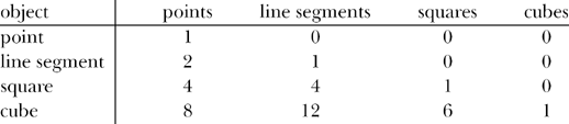
We start with a point and move it a certain distance—we can, with no loss of generality, take it to be the unit distance—along our first space dimension. The result is a single line segment with two end points, which we’ll call vertices. We follow this by a second motion, that is, we move the line segment a unit distance along our second space dimension, which is in a direction at right angles to our first motion. The result is a square, with four vertices and four line segments. What has happened is that our vertices have doubled, that is, each original vertex has duplicated itself. Also, our square has the original line segment, plus the original line segment in its new position, plus the two new line segments traced out by the motions of the original two vertices.

Next, we perform a third motion: we move the square a unit distance along our third space dimension which is at right angles to both of the first two motions. The result is a cube. Again, each of the square’s four vertices duplicates itself, and so the number of vertices in a cube is eight. Also, the number of line segments is equal to the original number (4), plus the original line segments in their final positions (4), plus the new line segments traced out by the motions of the original four vertices (4), for a total of twelve line segments. The number of square surfaces (faces) is the original surface (1), plus the original surface in its final position (1), plus the four new square surfaces traced out by the motion of the original number of line segments (4), for a total of six square surfaces. We can summarize all of this as above, where we read across a row to see, for a given object, how many points, line segments, squares, etc. are in that object:

If you think over the previous discussion you should be able to see how each entry, in each row, is generated by the following two rules: (1) the number of points in a n-dimensional cube is 2ⁿ and (2) all the other numbers in a row are twice the number directly above, plus the number directly to the left of the number just doubled. For example, the number of squares in a cube is 6 = 2 · 1 + 4. The value of these rules is that, using them, we can now construct the next row for a tesseract without having to move a cube unit distance along a fourth space dimension at right angles to the first three dimensions. (If you say you can visualize doing that, well, good for you—but I don’t believe it!) The result, for the tesseract, as you can easily confirm, is that it has sixteen vertices, thirty-two line segments, twenty-four square surfaces, and eight cubes. And once you have the tesseract row, you could keep right on going to generate the row for the 5-D cube and so learn that it has thirty-two vertices, eighty line segments, eighty square surfaces, forty cubes, and ten tesseracts!⁵ And then you could do the 6-D cube, the 7-D cube, … well, maybe I’m getting carried away here and we won’t do that. Back to business.

Now we know that the four-dimensional resistor cube has thirty-two resistors (a resistor for each line segment that forms an edge of the tesseract), but that doesn’t tell us how they are all connected together. For that, we turn next to binary numbers.

19.2 Connecting a Tesseract Resistor Cube

To see how to solve the connection problem, imagine you are A. Square in Flatland; how could he have figured out how a resistor cube in three dimensions is connected, even though he couldn’t “see” a three-dimensional object? Each of the eight vertices (or nodes) of the resistor cube can be located in three-dimensional space by specifying its coordinates, which will of course require three numbers, one for each dimension. Because we have constructed our cube out of motions of unit length along the various dimensions, all at right angles to each other, these numbers will be either 0 or 1, and so the coordinates of the eight nodes are the eight three-bit binary groups from (0,0,0) to (1,1,1, that is, we are numbering the nodes from 0 to 7.

Now, here’s the crucial observation: when we move from one node through a connecting resistor to the next node, we change just one of the bits in the initial binary group; for example, (0,0,0) is connected through a resistor to (0,0,1), through another resistor to (0,1,0), and through a third resistor to (1,0,0). Using this idea⁶ on all eight nodes in the cube, A. Square could have constructed the following connection wire list for the 3-D cube:

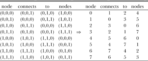
where it should be clear that node (0,0,0) = 0 and node (1,1,1) = 7 are opposite nodes, that is, body diagonal nodes. This last wire list is still not quite in the proper form for use by mccube.m, however, because it violates a couple of that code’s conventions. First, there can be no node 0; mccube.m assumes the numbering of the nodes starts with 1. And second, mccube.m wants to see nodes 1 and 2 as the body diagonal nodes (the nodes where the positive and negative terminals of the applied voltage source connect), not 0 and 7. Both of these transgressions are, fortunately, easy to fix. First, relabel 0 as 1 and 1 as 8. Second, relabel 7 as 2 and 2 as 7. That gives us the following final wire list:

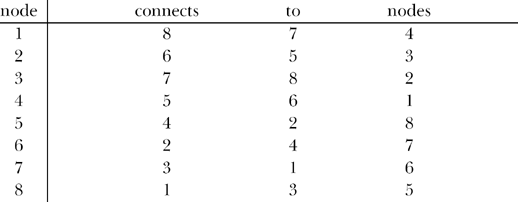
This wire list is what A. Square in Flatland could have constructed and, in fact, as Figure 19.1 shows, it does indeed correctly represent the connection of a 3-D cube. The nodes are not labeled as in Figure 17.3 (except for the convention of where nodes 1 and 2 have to be), but that just confirms what I stated in Discussion 17, that the labeling of all nodes other than 1 and 2 is arbitrary. Note carefully that A. Square does not need to actually draw Figure 19.1; I’ve included it here simply to illustrate that the binary method for constructing the cube’s wire list does indeed work. All that matters, however, all that A. Square needs, is the wire connection list.

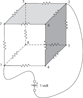
Figure 19.1. A square’s 3-D cube.

Now, to answer the question that opened this discussion—what is the body diagonal resistance of a 4-D resistor cube?—for the analogous problem faced by A. Square with the 3-D cube, he could next have fed mccube.m the above final wire list and used the code to find the voltages at nodes 3, 4, and 7, and so have calculated the input current from the one-volt voltage source to the cube as

The body diagonal resistance of a 3-D cube would then be

When I did this the result was R₃= 0.8336 ohms, which compares well with the theoretical result of 5/6 = 0.83333 ohms. Well, what A. Square could do⁷ in Flatland to find R₃ we can do in our world to find R₄.

I’ll begin as before, by writing the coordinates of the tesseract’s sixteen vertices as four-bit binary code groups from (0, 0, 0, 0) to (1, 1, 1, 1). Then, again as before, we can construct a preliminary connection wire list by examining where each code group “goes” as we successively change just one bit. This results in

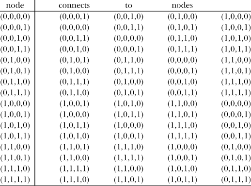
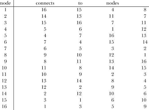
And again, because of the conventions of mccube.m, we must relabel 0 as 1 and 1 as 16, and also relabel 15 as 2 and 2 as 15; nodes 0 and 15, in our preliminary wire list, are opposite (body diagonal) nodes on the tesseract resistor cube, which must be (to keep mccube.m happy) labeled as nodes 1 and 2. This relabeling gives us our final wire list. (on next page)

Now, since node 1 is the positive terminal of an applied one-volt source, and since node 1 connects to nodes 4, 8, 15 and 16, then the input current to the tesseract is

and so the body diagonal resistance of a tesseract resistance cube made from one-ohm resistors is

When mccube.m was given this final wire list the result was R₄ = 0.6673 ohms. How good an estimate is this? It can be shown,⁸ using a symmetry argument that is a generalization of the one I used in Discussion 17 to calculate R₃, that the body diagonal resistance of an n-dimensional resistor cube made from one-ohm resistors is

For n = 3, for example,

which agrees with our earlier result. And for n = 4,

So, again, mccube.m has done well.

If you’re looking for a way to kill an afternoon, I’ll let you work through setting-up mccube.m for the resistor cube in the fifth dimension!⁹

Notes and References

1. Science fiction has, of course, had a lot of fun with the fourth dimension. For an extended discussion on this, see my book, Time Machines: Time Travel in Physics, Metaphysics, and Science Fiction 2nd ed. (New York: Springer, 1999, in particular Chapter 2 [“On the Nature of Time, Spacetime, and the Fourth Dimension”], pp. 97–178).

2. Edwin Abbott (1838–1926) was an English educator and theologian whose book, while on the surface about mathematical geometry in a plane, is actually a rather pointed critique of snobby Victorian society (for example, the more sides a regular n-gon has, the higher in social standing is that gon; regular ∞-gons or circles have the “ultimate” status). A similar literary experiment was published a few years later by H. G. Wells, in his even more famous and much darker “scientific romance” The Time Machine (1895). Wells’s motivation for “inventing” a time machine was simply that he needed a gadget to get his hero into the far future. Then he could come back to the present and report on the ultimate fate of the Victorian split between the poor and the rich (who would become the Morlocks and the Eloi, respectively), and to illustrate the horrors that that age’s smug optimism—that all was right with the world, and nothing needed to change—might produce. Flatland has had several imitators over the decades, some good and some not. I recommend the 1965 effort by the Dutch mathematical physicist Dionys Burger (1892–1987), Sphereland, supposedly written by A. Square’s grandson, “A. Hexagon.” (As explained in Flatland, a son always has one more side than does his father, and thus each new generation rises in social status simply as a birthright, and so that is, indeed, the correct name for a grandson.)

3. The procedure I’ll follow with this part of the discussion is based on the short essay by Ralph Milne Farley, “Visualizing Hyperspace” (Scientific American, March 1939, pp. 148–149), from which comes the quotation. This essay is well written, but many of its ideas had been around for decades; see Henry P. Manning, The Fourth Dimension Simply Explained, first published in 1910 (reprinted by Dover in 1960), which contains popular essays submitted to a 1909 contest sponsored by Scientific American. “Farley” was the pseudonym used by Roger Sherman Hoar (1887–1963), a Harvard-trained lawyer who once served as the assistant attorney general of Massachusetts. He adopted his pen name, apparently, to keep his science fiction writing (which was voluminous) separate from his legal writing (also voluminous). The irony in this comes from the fact that science fiction is the genre where he should have used his real name—that’s the stuff people remember today!

4. For what this means, see my book, An Imaginary Tale: The Story of (Princeton, N.J.: Princeton University Press, 1998, 2007, pp. 97–104).

5. If you initially balked at four-dimensional space, then you might think five-dimensional space to be really ludicrous, but that is not so. In 1921 the German physicist Theodor Kaluza (1885–1954) expanded the four-dimensional space-time of Einstein (3 space dimensions + 1 time dimension) to a five-dimensional space-time; he did that by adding a fourth space dimension. The result was that Maxwell’s electromagnetic field equations were an automatic conclusion of Einstein’s gravitational field equations, that is, Kaluza’s five dimension space-time unified electricity and gravity! The obvious question, of course, is just where is that extra space dimension? In 1926 the Swedish physicist Oskar Klein (1894–1977) speculated that it’s “curled up in a tiny circle, a concept you can read more about in an essay by Bryce S. DeWitt, “Quantum Gravity” (Scientific American, December 1983). Since the 1920s the so-called Kaluza-Klein theory has mutated into today’s controversial “string theories of everything” that require spaces with even more dimensions beyond the fifth.

6. This changing of a single bit as we move through one edge of the cube is called a Hamming distance of one, in honor of the American mathematician Richard Hamming (1915–1998). Hamming made great use of this simple idea to show how to generate binary codes that can both detect and self-correct random errors in the digital transmission of information. The self-correcting feature was long thought by many to be impossible until Hamming’s insight of motion in an n-dimensional space showed it was not only possible, but not even difficult. When I taught during my 1981–1982 sabbatical year at the Naval Postgraduate School in Monterey, California, where Hamming was on the computer science faculty, he was treated almost as a god. I was far too shy to exchange even a single word with him—something I regret to this day—but I often saw him walking across campus with a student entourage trailing after him and hanging on every utterance.

7. Notice that A. Square could have actually constructed a 3-D resistor cube in Flatland. That is, a 3-D cube can be collapsed into a planar circuit, with no edge of the cube crossing another edge. It wouldn’t “look like a cube anymore (but rather like two squares, one inside the other with analogous corner nodes connected together), but from a connection point of view it would still be a cube. However, A. Square could not have measured R₃ in Flatland by connecting a voltage source to the body diagonal nodes and measuring the resulting source current. That’s because one of the wires connecting the voltage source to the planar cube would have to cross a cube edge, and the only way to do that (to avoid a short circuit) is to “hop over” the blocking edge by using the third dimension. We, however, can measure R₄ because, after we’ve collapsed the tesseract into three dimensions, there is no concern of edges or connecting wires intersecting one another. You can find the schematic of a collapsed 4-D resistor cube used in an ELECTRONICS WORKBENCH simulation, in my book, The Science of Radio, 2nd ed. (New York: Springer, 2001, p. 376). As a final comment on collapsing, in Robert Heinlein’s story (see the second opening quotation), the “collapse” occurs in the opposite sense. That is, a California architect’s house, originally built in our 3-D spatial world but with all the collapsed connections of a tesseract, “uncollapses” into the 4-D spatial world when it is shaken by an earthquake!

8. O. J. Tretiak and T. S. Huang, “Resistance of an N-Dimensional Cube” (Proceedings of the IEEE, September 1965, pp. 1271–1272). The authors were not cranks. Both were at MIT, a known hothouse, then and now, for spectacular electrical engineering projects.

9. The answer is ohms.