Principal component analysis (PCA) is a statistical technique used for explaining the variance–covariance matrix of a set of m‐dimensional variables through a few linear combinations of these variables. In this chapter, we will illustrate the method to show that a large m‐dimensional process can often be sufficiently explained by smaller k principal components and thus reduce a higher dimension problem to one with fewer dimensions.

4.1 Introduction

Because of the advances of computing technology, the dimension, m, used in data analysis has become larger and larger. PCA is a statistical method that converts a set of correlated variables into a set of uncorrelated variables through an orthogonal transformation. Hopefully, a small subset of the uncorrelated variables carries sufficient information of the original large set of correlated variables.

The PCA concept to achieve parsimony was first introduced by Karl Pearson (1901). However, it was Hotelling (1933) who developed the method of stochastic variables and officially introduced the term of principal components in 1933. The techniques can be used on general variables or standardized variables and hence either the covariance matrix or correlation matrix. To many people, these techniques seem related, but in reality, they could be quite different. The goal of the method is to represent a large m‐dimensional process with much smaller k principal components and hence reduce a higher dimension problem to one with fewer dimensions.

We will begin with the population PCA, discuss its properties and interpretations, and then extend it to a sample PCA. We will also discuss the large sample properties of the sample principal components.

4.2 Population PCA

Given a m‐dimensional random vector Z = [Z₁,  …,  Z_m]′, let Σ be the covariance matrix,

where μ = E(Z_t). We will choose a vector such that Y₁ = α′Z has the maximum variance. Moreover, to obtain a unique solution, we also require that α′α = 1. That is, we will choose such that

(4.1)

Putting them together, we obtain the solution using the method of the Lagrange multiplier. That is, let

(4.2)

where λ is a Lagrange multiplier, and we maximize V with the constraint. Thus,

or

Since α ≠ 0, we have

That is, λ is an eigenvalue and α is the corresponding eigenvector of Γ, that is

(4.3)

In fact, because

this λ is actually the largest eigenvalue of Γ. We will call it λ₁ and its corresponding eigenvector as

Because Γ is m × m, there will be m such eigenvalues, λ₁ ≥ λ₂ ≥ ⋯ ≥ λ_m ≥ 0, and we denote the corresponding normalized eigenvectors as α₁, α₂, …, α_m, where Thus, we obtain the following linear combinations

(4.4)

such that

(4.5)

We will call the first principal component, the second principal component, and so on.

4.3 Implications of PCA

Let Λ be the diagonal matrix of eigenvalues and be the matrix formed from the corresponding normalized eigenvectors in the PCA. Since P′P = PP′ = I, Eq. (4.3) implies that

(4.6)

and

(4.7)

Since γ_i,i = Var(Z_i), i = 1, 2, …, m, we note that

(4.8)

The proportion of the total variance of Z_t explained by the ith principal component Y_i is given by

(4.9)

In many applications, the sum of the variances of the first few principal components may account for more than 85 or 90% of the total variance. This implies that the study of a given high m‐dimensional process Z can be accomplished through the careful study of a set containing a small number of principal components without losing much information.

Let e_i be the ith m‐dimensional unit vector with its ith element being 1 and 0 otherwise, for example, and In many applications, we may want to find the relationship between a principal component Y_i and variable Z_j in Z. It is interesting to note that

It follows that

(4.10)

for i, j = 1, 2, …, m. Thus, one can use the relative magnitude of the correlations or the coefficients α_i,j associated with variable Z_j to interpret the principal components. These correlations and coefficients together with their positive or negative signs can also be used to measure the importance of the variables in Z to a given principal component. They sometimes lead to different rankings, but they often reach similar results.

In these discussions, we obtain principal components for a given process Z through its variance–covariance matrix Γ. Clearly, we can also construct these principal components through its correlation matrix,

(4.11)

where D is the diagonal matrix in which the ith diagonal element is the variance of the ith process, that is

(4.12)

In other words, we will construct the principal components for the standardized variables,

(4.13)

and ρ is the covariance matrix of U because Cov(U) = D^−1/2ΓD^−1/2 = ρ. Hence, the procedure of constructing the principal components from these standardized variables is exactly the same as before. The first natural question to ask is, why do we use standardized variables? One obvious answer is that in many applications the unit used in variables may not be the same. For example, if values of one variable are mostly small numbers between 0 and 1 like percentages but values of one other variable are mostly numbers in the millions or billions like imports and exports, then to avoid the unnecessary impact of the different units used in these variables, we will naturally consider using standardized variables. The second question to ask is, are the two sets of principal components constructed from Γ and ρ the same? The unfortunate answer is decidedly no. In fact, they could be very different. The choice depends on applications and could be a challenge in applied research.

4.4 Sample principle components

In practice, we may not know the parameter value Γ of Z. So, given a m‐dimensional stationary vector time series Z_t, we will simply replace the unknown population variance–covariance matrix, Γ, by the sample variance–covariance matrix, computed from Z_t, t = 1, 2, …, n,

(4.14)

where

• is the sample mean vector,
• is the sample variance of the Z_i,
• is the sample covariance between Z_i and Z_j.

In exactly the same approach, we will now choose a vector such that has the maximum sample variance, where we denote the vector and its resulting linear combination with a hat for distinction between the population and sample principal components. Thus, the first sample principal component will be obtained by

The second sample principal component will be obtained by

and zero sample covariance between and

Continuing, the ith sample principal component will be obtained by

Let be the eigenvalue–eigenvector pairs of the sample variance–covariance matrix, The ith sample principal component is in fact given by

where From the process and the results from Sections 4.2 and 4.3, we have

1. 
2. Sample covariance between is zero for i ≠ j.
3. 
4. Sample covariance between
5. Sample correlation between

Similar to the population principal components, we can obtain the sample principal components through the sample variance–covariance matrix or the sample correlation matrix,

(4.15)

where is the diagonal matrix in which the ith diagonal element is the sample variance of Z_{i, t}, that is

(4.16)

In other words, we will construct the sample principal components for the standardized sample variables,

(4.17)

and is the sample covariance matrix of The procedure is exactly the same as before. For simplicity, we will use the same notations, for the sample principal components and their associated eigenvalues and eigenvectors irrespective of whether they are constructed from Whether from should be clear from the applications. Again, the two sets of sample principal components constructed from will in general be different. The choice depends on applications.

Once the sample principal components are obtained, the next natural step is to investigate their properties through Their large sample properties are summarized in the following theorem, and we refer readers to Anderson (1963) for its proof. We also refer readers to reference books by Johnson and Wichern (2002), and Rao (2002).

The result in (1) implies that the values are independently normally distributed as N(λ_i, 2λ_i/n). Hence, the 100(1 − α)% confidence interval for λ_i can be obtained as follows:

(4.19)

where N_α/2 is the upper 100(α/2)th percentile of the standard normal distribution.

From these discussions, it is clear that PCA is a statistical method used to find k linear combinations of m original statistical variables through the analysis of the covariance or correlation matrix of these m variables with k being much less than m, so that the study of a given high m‐dimensional process can be accomplished through the study of a much smaller number of principal components without losing much information. Obviously, this makes sense only when the covariance and correlation is stable and constant. Hence, for a time series process, it has to be stationary. For a nonstationary series, it needs to be reduced to stationary by using some transformations such as power transformation and differencing. Since the residual vector, a_t, is actually a function of Z_t, one can also analyze the covariance or correlation matrix of residuals after a VAR model fitting. Also, when using PCA, we normally work on a mean adjusted data set.

4.5 Empirical examples

4.5.1 Daily stock returns from the first set of 10 stocks

4.5.1.1 The PCA based on the sample covariance matrix

The eigenvalues and eigenvectors, which are often known as variances and component loadings, of the sample variance–covariance matrix, are given in Table 4.1.

	Comp. 1	Comp. 2	Comp. 3	Comp. 4	Comp. 5	Comp. 6	Comp. 7	Comp. 8	Comp. 9	Comp. 10
CVX	−0.166	−0.104	−0.407	0.576	0.120				0.622	−0.227
XOM	−0.230	−0.126	−0.243	0.552		0.203			−0.686	0.215
AAPL		−0.431	−0.173	−0.354	0.180	0.377	−0.639	−0.264
FB		−0.513	−0.319	−0.231	−0.324	−0.213	0.505	−0.399
MSFT		−0.362	−0.286	−0.197	0.127	−0.116		0.841
MRK	−0.470	−0.329	0.596		0.396	0.223	0.320
PFE	−0.369	−0.167	0.316	0.126	−0.725	−0.118	−0.358	0.136		−0.165
BAC	−0.539	0.289	−0.191	−0.222	0.279	−0.438	−0.164	−0.155	−0.217	−0.416
JPM	−0.391	0.175				−0.206			0.265	0.827
WFC	−0.324	0.379	−0.251	−0.265	−0.266	0.678	0.255			−0.110
Variance	0.00058	0.00030	0.00018	0.00011	0.00009	0.00008	0.00007	0.00005	0.00003	0.00002
Percentage of Total Variance	0.384	0.199	0.119	0.073	0.060	0.053	0.046	0.033	0.020	0.013

Figure 4.2 shows a useful plot, which is often known as a scree plot or screeplot. It is a plot of eigenvalues versus i, that is, the magnitude of an eigenvalue versus its number. To determine the suitable number, k, of components, we look for an elbow in the plot, where the component preceding the vertex of the elbow is chosen to be cutoff point k. In our example, we will choose k to be 3 or 4.

The eigenvalues of the first four components account for

of the total sample variance.

The four sample principal components are

Now, let us examine the four components more carefully. The first component represents the general market other than communication technology sector. The second component represents the contrast between financial and non‐financial sectors. The third component represents the contrast between health and non‐health sectors. The fourth component represents the contrast between oil and non‐oil industries. Thus, the PCA has provided us with four components that contain a vast amount of information for the 10 stock returns traded on the New York Stock Exchange.

4.5.1.2 The PCA based on the sample correlation matrix

Now let us try the PCA using the sample correlation matrix, which is based on the standardized variables,

The eigenvalues and eigenvectors, which are also known as variances and component loadings, of the sample correlation matrix are given in Table 4.2. The screeplot is shown in Figure 4.3.

	Comp. 1	Comp. 2	Comp. 3	Comp. 4	Comp. 5	Comp. 6	Comp. 7	Comp. 8	Comp. 9	Comp. 10
CVX	−0.287	−0.155	0.654	−0.136			0.287		0.578	−0.150
XOM	−0.354	−0.137	0.464	−0.320	0.187		−0.319	0.116	−0.598	0.146
AAPL		−0.491	−0.199	0.233	0.744	−0.192	0.163	−0.204
FB	−0.143	−0.506		0.171	−0.517	−0.416	0.355	0.308	−0.167
MSFT	−0.150	−0.490		0.341	−0.241	0.493	−0.539	−0.131	0.102
MRK	−0.346		−0.418	−0.405	0.164	0.318		0.602	0.207
PFE	−0.364		−0.354	−0.429	−0.198	−0.367	−0.217	−0.538	0.143	−0.166
BAC	−0.433	0.236		0.281		0.258	0.310	−0.121	−0.367	−0.602
JPM	−0.458	0.231		0.206		0.154	0.238	−0.210		0.747
WFC	−0.310	0.320		0.458	0.144	−0.457	−0.415	0.342	0.269
Variance	3.393	2.210	1.196	0.939	0.557	0.504	0.406	0.378	0.296	0.121
Cumulative % of Total Variance	33.93%	56.03%	67.99%	77.38%	82.85%	87.99%	92.95	95.83%	98.79%	100%

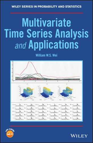
The screeplot again indicates k = 4. The eigenvalues of the first four components account for

which is almost the same as the one obtained using the covariance matrix. The four sample principal components are now

Now, let us examine the four components. The first component now represents the general stock market. The second component represents the contrast mainly between financial and non‐health related sectors. The third component represents the contrast between oil and health sectors. The fourth component now represents the contrast between financial/technology and non‐financial/non‐technology industry. For this data set, the PCA results from the covariance matrix and the correlation matrix are very much equivalent.

4.5.2 Monthly Consumer Price Index (CPI) from five sectors

4.5.2.1 The PCA based on the sample covariance matrix

The eigenvalues and eigenvectors, which are often known as variances and component loadings of the sample variance–covariance matrix, are given in Table 4.3.

	Comp. 1	Comp. 2	Comp. 3	Comp. 4	Comp. 5
Energy	0.516	0.081	−0.301	0.782	−0.158
Apparel	0.003	−0.057	0.859	0.398	0.318
Commodities	0.227	−0.331	0.354	−0.148	−0.832
Housing	0.461	−0.755	−0.117	−0.187	0.411
Gas	0.686	0.557	0.184	−0.415	0.118
Variance	11 068.83	379.65	89.84	18.11	2.70
Proportion of total variance explained by ith component	0.9576	0.0328	0.0078	0.0016	0.0002

The two sample principal components are

The first component explains 95.76% of the total sample variance, and the first two explain 99.04%. Thus, sample variation is very much summarized by the first principle component or the first two principle components. Figure 4.5 shows the useful screeplot where the vertex of the elbow can be easily seen to be k = 1.

Now, let us examine component 1 more carefully. In this component, the loadings are all positive. The component can be regarded as the CPI growth component that grew over the time period that we observed. The five variables are combined into a composite score, which is plotted in Figure 4.6, and it follows a combination of patterns observed mainly for gasoline and energy in Figure 4.4.

Thus, the PCA has provided us with a single component that contains the vast majority of information for the five individual variables. From this, we can conclude that gasoline and energy were the true drivers of the overall economy for the Greater New York City area during the period between 1986 and 2014.

4.5.2.2 The PCA based on the sample correlation matrix

Now let us try the PCA using the sample correlation matrix. The eigenvalues and eigenvectors, which are also known as variances and component loadings, of the sample correlation matrix are given in Table 4.4.

	Comp. 1	Comp. 2	Comp. 3	Comp. 4	Comp. 5
Energy	0.503	0.100	0.322	0.676	−0.420
Apparel	0.044	−0.987	0.100	0.103	0.060
Commodities	0.501	−0.107	−0.417	−0.505	−0.556
Housing	0.499	0.032	−0.550	0.267	0.614
Gas	0.495	0.061	0.641	−0.455	0.366
Variance	3.837	1.018	0.135	0.008	0.002
Proportion of total variance explained by ith component	0.7674	0.2036	0.027	0.0016	0.0004

The two sample principal components are

The first component explains 76.74% of the total sample variance, and the first two explain 97.1%. Thus, sample variation of the five industries is primarily summarized by the first two principle components. Figure 4.7 shows the screeplot, which clearly indicates k = 2.

From Table 4.4, we see that the loadings in component 1 are all positive, almost equal for energy, commodities, housing, and gas, and have strong positive correlations among them. It represents the CPI growth over the time period that we observed. The loadings in component 2 are relatively positive small numbers for energy, housing, and gas, and negative for apparel and commodities. It represents the market contrast between consumer goods and utility housing. Since the loading for apparel is especially dominating, component 2 can also be simply regarded as representing the apparel sector.

The five variables are combined into two composite scores, which are plotted in Figure 4.8.

The plots of component 1 based on sample covariance matrix and sample correlation matrix as shown in Figures 4.6 and 4.8 are almost the same. However, the proportion of total variance explained by component 1 is 96% when the original variables are used and 77% when the standardized variables are used. As shown in the example, the PCA results from the covariance matrix and the correlation matrix could be different.

For further information on PCA and applications, we refer readers to Joyeux (1992), Cubadda (1995), Ait‐Sahalia and Xiu (2017), Estrada and Perron (2017), Jandarov et al. (2017), Passemier et al. (2017), Sang et al. (2017), and Zhu et al. (2017), among others.

Projects

1. Find a multivariate analysis book and carefully read its chapter on PCA.
2. Find an m‐dimensional social science related time series data set with m ≥ 6. Construct your principle component model based on its sample covariance matrix and evaluate your findings with a written report and analysis software code.
3. For the data set in Project 2, construct your principle component model based on its sample correlation matrix, and compare your result with that in Project 2. Write a report on your findings with associated software code.
4. Find an m‐dimensional natural science related data set with m ≥ 6. Construct your principle component model based on its sample covariance and correlation matrices separately, and evaluate your findings with a written report and analysis software code.
5. Find an m‐dimensional time series data set of your interest with m ≥ 10. Construct your principle component model based on its sample covariance and correlation matrices separately, and evaluate your findings with a written report and analysis software code.

References

1. Ait‐Sahalia, Y. and Xiu, D. (2018). Principal component analysis of high frequency data. Journal of American Statistical Association 11–14. https://doi.org/10.1080/01621459.2017.1401542.
2. Anderson, T.W. (1963). Asymptotic theory for principal components analysis. Annals of Mathematical Statistics 34: 122–148.
3. Cleveland, R.B., Cleveland, W.S., McRae, J.E., and Terpenning, I. (1990). A seasonal‐trend decomposition procedure based on loess (with discussion). Journal of Official Statistics 6: 3–73.
4. Cubadda, G. (1995). A note on testing for seasonal cointegration using principal components in the frequency domain. Journal of Time Series Analysis 16: 499–508.
5. Estrada, F. and Perron, P. (2017). Extracting and analyzing the warming trend in global and hemispheric temperatures. Journal of Time Series Analysis 38: 711–732.
6. Hotelling, H. (1933). Analysis of a complex of statistical variables into principle components. Journal of Educational Psychology 24: 417–441. 498−520.
7. Jandarov, R.A., Sheppard, L.A., Sampson, P.D., and Szpiro, A.A. (2017). A novel principal component analysis for spatially misaligned multivariate air pollution data. Journal of Statistical Society, Series C 66: 3–28.
8. Johnson, R.A. and Wichern, D.W. (2002). Applied Multivariate Statistical Analysis, 5e. Prentice Hall.
9. Joyeux, R. (1992). Testing for seasonal cointegration using principal components. Journal of Time Series Analysis 13: 109–118.
10. Passemier, D., Li, Z., and Yao, J. (2017). On estimation of the noise variance in high dimensional probabilistic principal component analysis. Journal of Royal Statistical Society, Series B 79: 51–67.
11. Pearson, K. (1901). On lines and planes of closest fit to systems of points in space. Philosophical Magazine, 6^th Series II: 559–572.
12. Rao, C.R. (2002). Linear Statistical Inference and Its Applications, 2e. Wiley.
13. Sang, T., Wang, L., and Cao, J. (2017). Parametric functional principal component analysis. Biometrics 73: 802–810.
14. Zhu, H., Shen, D., Peng, X., and Liu, L.Y. (2017). MWPCR: multiscale weighted principal component regression for high‐dimensional prediction. Journal of American Statistical Association 112: 1009–1021.