Empirical Example 9.4 of nonstationary vector time series – analysis of financial data
function [f,gr,h] = Beta_derive1(x, yobs_tmp, chol_index, Phi_temp, tau_temp,...
Beta_temp, sigmasqalpha, nbasis)
global dimen
%%%%%%%%%%%%%%%%%%%%%%%%%%%%%%%%%%%%%%%%%%%%%%%%%%%%%%%%%%%%%%%%%%%%%%%%%%%%%%%
% Function used for optimization process for coefficients selected to % be changed
%
% Input:
% 1) x - initial values for coefficient of basis functions need to % be optimized
% 2) yobs_tmp - time series data within the segment
% 3) chol_index - index matrix
% 4) Phi_temp - which component changed
% 5) tau_temp - smoothing parameters
% 6) Beta_temp - current coefficients
% 7) sigmasqalpha - smoothing parameters for the constant in real % components
% 8) nbasis - number of basis functions used
% Main Outputs:
% 1) f - log posterior probability based on input parameters
% 2) gr - gradients for optimization process
% 3) h - Hessian matrix for optimization process
%
% Required programs: lin_basis_func
%%%%%%%%%%%%%%%%%%%%%%%%%%%%%%%%%%%%%%%%%%%%%%%%%%%%%%%%%%%%%%%%%%%%%%%%%%%%%%%
%initilize Beta_1 and Beta_2: Beta_2 is for imaginary components
nBeta = nbasis + 1;
Beta_1 = zeros(nBeta,(dimen + dimen*(dimen-1)/2));
Beta_2 = zeros(nBeta,dimen*(dimen-1)/2);
select = chol_index(Phi_temp,:).*(1:dimen^2);
select = select(select∼=0);
x = reshape(x,nBeta,length(select));
Beta_temp(:,select) = x;
Beta_1(:,:) = Beta_temp(:,1:(dimen + dimen*(dimen-1)/2));
Beta_2(:,:) = Beta_temp(1:nBeta,(dimen + dimen*(dimen-1)/2 + 1): end);
dim = size(yobs_tmp); n = dim(1);
nfreq = floor(n/2); tt = (0:nfreq)/(2*nfreq);
yy = fft(yobs_tmp)/sqrt(n); y = yy(1:(nfreq+1),:); nf = length(y);
[xx_r, xx_i]=lin_basis_func(tt);
%theta's
theta = zeros(dimen*(dimen-1)/2,nf);
for i=1:dimen*(dimen-1)/2
theta_real = xx_r * Beta_1(:,i+dimen);
theta_imag = xx_i * Beta_2(:,i);
theta(i,:) = theta_real + sqrt(-1)*theta_imag;
end
%delta's
delta_sq = zeros(dimen,nf);
for i=1:dimen
delta_sq(i,:) = exp(xx_r * Beta_1(:,i));
end
if dimen==2 %Bivariate Time Series
if (mod(n,2)==1)%odd n
f = -sum(log(delta_sq(1,2:end))' + log(delta_sq(2,2:end))' + abs(y(2:end,1)).^2.*exp(-xx_r(2:end,:)*Beta_1(:,1)) + ...
abs(y(2:end,2) - theta(2:end).'.*y(2:end,1)).^2.*exp(-xx_r(2:end,:)*Beta_1(:,2))) - ...
0.5*(log(delta_sq(1,1))' + log(delta_sq(2,1))' + abs(y(1,1)).^2.*exp(-xx_r(1,:)*Beta_1(:,1)) + ...
abs(y(1,2) - theta(1).'.*y(1,1))^2.*exp(-xx_r(1,:)*Beta_1(:,2)));
else
f = -sum(log(delta_sq(1,2:nfreq))' + log(delta_sq(2,2:nfreq))' + abs(y(2:nfreq,1)).^2.*exp(-xx_r(2:nfreq,:)*Beta_1(:,1)) + ...
abs(y(2:nfreq,2) - theta(2:nfreq).'.*y(2:nfreq,1)).^2.*exp(-xx_r(2:nfreq,:)*Beta_1(:,2))) - ...
0.5*(log(delta_sq(1,1)) + log(delta_sq(2,1)) + abs(y(1,1)).^2.*exp(-xx_r(1,:)*Beta_1(:,1)) + ...
abs(y(1,2) - theta(1).'.*y(1,1)).^2.*exp(-xx_r(1,:)*Beta_1(:,2))) - ...
0.5*(log(delta_sq(1,end)) + log(delta_sq(2,end)) + abs(y(end,1)).^2.*exp(-xx_r(end,:)*Beta_1(:,1)) + ...
abs(y(end,2) - theta(end).'.*y(end,1))^2.*exp(-xx_r(end,:)*Beta_1(:,2)));
end
f = f - (0.5.*(Beta_1(1,1)* Beta_1(1,1)')/sigmasqalpha + 0.5.*(Beta_1(2:nBeta,1)'*Beta_1(2:nBeta,1))/tau_temp(1))*chol_index(Phi_temp,1) -...
(0.5.*(Beta_1(1,2)* Beta_1(1,2)')/sigmasqalpha + 0.5.*(Beta_1(2:nBeta,2)'*Beta_1(2:nBeta,2))/tau_temp(2))*chol_index(Phi_temp,2) -...
(0.5.*(Beta_1(1,3)* Beta_1(1,3)')/sigmasqalpha + 0.5.*(Beta_1(2:nBeta,3)'*Beta_1(2:nBeta,3))/tau_temp(3))*chol_index(Phi_temp,3) -...
(0.5.*(Beta_2(1:nBeta,1)'*Beta_2(1:nBeta,1))/tau_temp(4))*chol_index(Phi_temp,4);
gr1 = zeros(nBeta,1); gr2 = zeros(nBeta,1); gr3 = zeros(nBeta,1); gr4 = zeros(nBeta,1);
gr1(1) = Beta_1(1,1)/sigmasqalpha; gr1(2:nBeta,1) = Beta_1(2:nBeta,1)/tau_temp(1);
gr2(1) = Beta_1(1,2)/sigmasqalpha; gr2(2:nBeta,1) = Beta_1(2:nBeta,2)/tau_temp(2);
gr3(1) = Beta_1(1,3)/sigmasqalpha; gr3(2:nBeta,1) = Beta_1(2:nBeta,3)/tau_temp(3);
gr4(1:nBeta,1) = Beta_2(1:nBeta,1)/tau_temp(4);
h11(1,1)=1/sigmasqalpha; h11(2:nBeta,2:nBeta)=1/tau_temp(1)*eye(nbasis);
h22(1,1)=1/sigmasqalpha; h22(2:nBeta,2:nBeta)= 1/tau_temp(2)*eye(nbasis);
h33(1,1)=1/sigmasqalpha; h33(2:nBeta,2:nBeta)= 1/tau_temp(3)*eye(nbasis);
h44(1:nBeta,1:nBeta)=1/tau_temp(4)*eye(nBeta);
h42 = zeros(nBeta,nBeta); h32 = zeros(nBeta,nBeta);
if (mod(n,2)==1)
%%%%%%%%%%%%%%%%%%%%%%%%%%%%%%%%%%%%%%%
%gradient
%%%%%%%%%%%%%%%%%%%%%%%%%%%%%%%%%%%%%%%
rk = -y(2:end,1).*conj(y(2:end,2)) - y(2:end,2).*conj(y(2:end,1));
ik = sqrt(-1)*(-y(2:end,1).*conj(y(2:end,2)) + y(2:end,2).*conj(y(2:end,1)));
ck = 2*abs(y(2:end,1)).^2;
gr1 = gr1 + xx_r(2:end,:)'*(1-abs(y(2:end,1)).^2.*exp(-xx_r(2:end,:)*Beta_1(:,1))) + ...
0.5*(xx_r(1,:)'*(1-abs(y(1,1)).^2.*exp(-xx_r(1,:)*Beta_1(:,1))));
gr2 = gr2 + xx_r(2:end,:)'*(1 - abs(y(2:end,2)-theta(2:end).'.*y(2:end,1)).^2.*exp(-xx_r(2:end,:)*Beta_1(:,2))) + ...
0.5*(xx_r(1,:)'*(1 - abs(y(1,2)-theta(1).'.*y(1,1)).^2.*exp(-xx_r(1,:)*Beta_1(:,2))));
temp_mat_31 = bsxfun(@times, xx_r(2:end,:),rk);
temp_mat_32 = bsxfun(@times, ck, bsxfun(@times, xx_r(2:end,:),xx_r(2:end,:)*Beta_1(:,3)));
gr3 = gr3 + sum( bsxfun(@times, (temp_mat_31+temp_mat_32), exp(-xx_r(2:end,:)*Beta_1(:,2)) ))' +...
0.5*(exp(-xx_r(1,:)*Beta_1(:,2))*(-y(1,1).*conj(y(1,2)) - y(1,2).*conj(y(1,1)))*xx_r(1,:)' +...
exp(-xx_r(1,:)*Beta_1(:,2))*2*abs(y(1,1)).^2*(xx_r(1,:)*Beta_1(:,3))*xx_r(1,:)');
temp_mat_41 = bsxfun(@times, ik, xx_i(2:end,:));
temp_mat_42 = bsxfun(@times, ck, bsxfun(@times,xx_i(2:end,:),xx_i(2:end,:)*Beta_2(:,1)));
gr4 = gr4 + sum( bsxfun(@times, (temp_mat_41 + temp_mat_42), exp(-xx_r(2:end,:)*Beta_1(:,2))))' + ...
0.5*(exp(-xx_r(1,:)*Beta_1(:,2))*(sqrt(-1)*(-y(1,1).*conj(y(1,2)) + y(1,2).*conj(y(1,1))))*xx_i(1,:)' +...
exp(-xx_r(1,:)*Beta_1(:,2))*2*abs(y(1,1)).^2*(xx_i(1,:)*Beta_2(:,1))*xx_i(1,:)');
%%%%%%%%%%%%%%%%%%%%%%%%%%%%%%%%%%%%%%%%
%Hessian
%%%%%%%%%%%%%%%%%%%%%%%%%%%%%%%%%%%%%%%%
bigmat_h11 = kron(bsxfun(@times, abs(y(2:end,1)).^2.*exp(-xx_r(2:end,:)*Beta_1(:,1)), xx_r(2:end,:)),ones(nBeta,1)');
coefmat_h11 = repmat(xx_r(2:end,:), 1,nBeta);
h11 = h11 + reshape(sum(bsxfun(@times, bigmat_h11, coefmat_h11),1),nBeta,nBeta) +...
0.5*(abs(y(1,1)).^2.*exp(-xx_r(1,:)*Beta_1(:,1))*xx_r(1,:)'*xx_r(1,:));
bigmat_h22 = kron(bsxfun(@times, abs(y(2:end,2)-theta(2:end).'.*y(2:end,1)).^2.*exp(-xx_r(2:end,:)*Beta_1(:,2)),...
xx_r(2:end,:)), ones(nBeta,1)');
coefmat_h22 = repmat(xx_r(2:end,:), 1,nBeta);
h22 = h22 + reshape(sum(bsxfun(@times, bigmat_h22, coefmat_h22),1),nBeta,nBeta) +...
0.5*(abs(y(1,2)-theta(1).'.*y(1,1)).^2.*exp(-xx_r(1,:)*Beta_1(:,2))*xx_r(1,:)'*xx_r(1,:));
bigmat_h33 = kron(bsxfun(@times, exp(-xx_r(2:end,:)*Beta_1(:,2)).*ck, xx_r(2:end,:)),ones(nBeta,1)');
coefmat_h33 = repmat(xx_r(2:end,:), 1,nBeta);
h33 = h33 + reshape(sum(bsxfun(@times, bigmat_h33, coefmat_h33),1),nBeta,nBeta) +...
0.5*(exp(-xx_r(1,:)*Beta_1(:,2))*2*abs(y(1,1)).^2*xx_r(1,:)'*xx_r(1,:));
bigmat_h44 = kron(bsxfun(@times, exp(-xx_r(2:end,:)*Beta_1(:,2)).*ck, xx_i(2:end,:)),ones(nBeta,1)');
coefmat_h44 = repmat(xx_i(2:end,:), 1,nBeta);
h44 = h44 + reshape(sum(bsxfun(@times, bigmat_h44, coefmat_h44),1),nBeta,nBeta) +...
0.5*(exp(-xx_r(1,:)*Beta_1(:,2))*2*abs(y(1,1)).^2*xx_i(1,:)'*xx_i(1,:));
bigmat_h42_1 = kron(bsxfun(@times, exp(-xx_r(2:end,:)*Beta_1(:,2)).*ck.*(xx_i(2:end,:)*Beta_2(:,1)),...
xx_i(2:end,:)), ones(nBeta,1)');
coefmat_h42_1 = repmat(xx_r(2:end,:), 1,nBeta);
bigmat_h42_2 = kron(bsxfun(@times,exp(-xx_r(2:end,:)*Beta_1(:,2)).*ik, xx_i(2:end,:)), ones(nBeta,1)');
coefmat_h42_2 = repmat(xx_r(2:end,:), 1,nBeta);
h42 = h42 + reshape(sum(bsxfun(@times, bigmat_h42_1, coefmat_h42_1) +...
bsxfun(@times, bigmat_h42_2, coefmat_h42_2),1),nBeta,nBeta)' +...
0.5*(exp(-xx_r(1,:)*Beta_1(:,2))*(2*abs(y(1,1)).^2*(xx_i(1,:)*Beta_2(:,1))*xx_i(1,:)+...
sqrt(-1)*(-y(1,1).*conj(y(1,2)) + y(1,2).*conj(y(1,1)))*xx_i(1,:))'*xx_r(1,:));
bigmat_h32_1 = kron(bsxfun(@times, exp(-xx_r(2:end,:)*Beta_1(:,2)).*ck.*(xx_r(2:end,:)*Beta_1(:,3)),...
xx_r(2:end,:)), ones(nBeta,1)');
coefmat_h32_1 = repmat(xx_r(2:end,:), 1,nBeta);
bigmat_h32_2 = kron(bsxfun(@times,exp(-xx_r(2:end,:)*Beta_1(:,2)).*rk, xx_r(2:end,:)), ones(nBeta,1)');
coefmat_h32_2 = repmat(xx_r(2:end,:), 1,nBeta);
h32 = h32 + reshape(sum(bsxfun(@times, bigmat_h32_1, coefmat_h32_1) +...
bsxfun(@times, bigmat_h32_2, coefmat_h32_2),1),nBeta,nBeta)' +...
0.5*(exp(-xx_r(1,:)*Beta_1(:,2))*(2*abs(y(1,1)).^2*(xx_r(1,:)*Beta_1(:,3))*xx_r(1,:)+...
(-y(1,1).*conj(y(1,2)) - y(1,2).*conj(y(1,1)))*xx_r(1,:))'*xx_r(1,:));
h24=h42'; h23=h32';
else
%%%%%%%%%%%%%%%%%%%%%%%%%%%%%%
%gradient
%%%%%%%%%%%%%%%%%%%%%%%%%%%%%%
rk = -y(2:nfreq,1).*conj(y(2:nfreq,2)) - y(2:nfreq,2).*conj(y(2:nfreq,1));
ik = sqrt(-1)*(-y(2:nfreq,1).*conj(y(2:nfreq,2)) + y(2:nfreq,2).*conj(y(2:nfreq,1)));
ck = 2*abs(y(2:nfreq,1)).^2;
gr1 = gr1 + xx_r(2:nfreq,:)'*(1-abs(y(2:nfreq,1)).^2.*exp(-xx_r(2:nfreq,:)*Beta_1(:,1))) + ...
0.5*(xx_r(1,:)'*(1-abs(y(1,1)).^2.*exp(-xx_r(1,:)*Beta_1(:,1)))) +...
0.5*(xx_r(end,:)'*(1-abs(y(end,1)).^2.*exp(-xx_r(end,:)*Beta_1(:,1))));
gr2 = gr2 + xx_r(2:nfreq,:)'*(1 - abs(y(2:nfreq,2)-theta(2:nfreq).'.*y(2:nfreq,1)).^2.*exp(-xx_r(2:nfreq,:)*Beta_1(:,2))) + ...
0.5*(xx_r(1,:)'*(1 - abs(y(1,2)-theta(1).'.*y(1,1)).^2.*exp(-xx_r(1,:)*Beta_1(:,2)))) + ...
0.5*(xx_r(end,:)'*(1 - abs(y(end,2)-theta(end).'.*y(end,1)).^2.*exp(-xx_r(end,:)*Beta_1(:,2))));
temp_mat_31 = bsxfun(@times,rk, xx_r(2:nfreq,:));
temp_mat_32 = bsxfun(@times,ck,bsxfun(@times, xx_r(2:nfreq,:),xx_r(2:nfreq,:)*Beta_1(:,3)));
gr3 = gr3 + sum(bsxfun(@times, (temp_mat_31 + temp_mat_32), exp(-xx_r(2:nfreq,:)*Beta_1(:,2)) ))' +...
0.5*(exp(-xx_r(1,:)*Beta_1(:,2))*(-y(1,1).*conj(y(1,2)) - y(1,2).*conj(y(1,1)))*xx_r(1,:)' +...
exp(-xx_r(1,:)*Beta_1(:,2))*2*abs(y(1,1)).^2*(xx_r(1,:)*Beta_1(:,3))*xx_r(1,:)') +...
0.5*(exp(-xx_r(end,:)*Beta_1(:,2))*(-y(end,1).*conj(y(end,2)) - y(end,2).*conj(y(end,1)))*xx_r(end,:)' +...
exp(-xx_r(end,:)*Beta_1(:,2))*2*abs(y(end,1)).^2*(xx_r(end,:)*Beta_1(:,3))*xx_r(end,:)');
temp_mat_41 = bsxfun(@times, ik, xx_i(2:nfreq,:));
temp_mat_42 = bsxfun(@times, ck, bsxfun(@times,xx_i(2:nfreq,:),xx_i(2:nfreq,:)*Beta_2(:,1)));
gr4 = gr4 + sum( bsxfun(@times, (temp_mat_41 + temp_mat_42), exp(-xx_r(2:nfreq,:)*Beta_1(:,2))))' + ...
0.5*(exp(-xx_r(1,:)*Beta_1(:,2))*(sqrt(-1)*(-y(1,1).*conj(y(1,2)) + y(1,2).*conj(y(1,1))))*xx_i(1,:)' +...
exp(-xx_r(1,:)*Beta_1(:,2))*2*abs(y(1,1)).^2*(xx_i(1,:)*Beta_2(:,1))*xx_i(1,:)') +...
0.5*(exp(-xx_r(end,:)*Beta_1(:,2))*(sqrt(-1)*(-y(end,1).*conj(y(end,2)) + y(end,2).*conj(y(end,1))))*xx_i(end,:)' +...
exp(-xx_r(end,:)*Beta_1(:,2))*2*abs(y(end,1)).^2*(xx_i(end,:)*Beta_2(:,1))*xx_i(end,:)');
%%%%%%%%%%%%%%%%%%%%%%%%%%%%%%%%%
%Hessian
%%%%%%%%%%%%%%%%%%%%%%%%%%%%%%%%%
bigmat_h11 = kron(bsxfun(@times, abs(y(2:nfreq,1)).^2.*exp(-xx_r(2:nfreq,:)*Beta_1(:,1)), xx_r(2:nfreq,:)),ones(nBeta,1)');
coefmat_h11 = repmat(xx_r(2:nfreq,:), 1,nBeta);
h11 = h11 + reshape(sum(bsxfun(@times, bigmat_h11, coefmat_h11),1),nBeta,nBeta) +...
0.5*(abs(y(1,1)).^2.*exp(-xx_r(1,:)*Beta_1(:,1))*xx_r(1,:)'*xx_r(1,:))+...
0.5*(abs(y(end,1)).^2.*exp(-xx_r(end,:)*Beta_1(:,1))*xx_r(end,:)'*xx_r(end,:));
bigmat_h22 = kron(bsxfun(@times, abs(y(2:nfreq,2)-theta(2:nfreq).'.*y(2:nfreq,1)).^2.*exp(-xx_r(2:nfreq,:)*Beta_1(:,2)),...
xx_r(2:nfreq,:)), ones(nBeta,1)');
coefmat_h22 = repmat(xx_r(2:nfreq,:), 1,nBeta);
h22 = h22 + reshape(sum(bsxfun(@times, bigmat_h22, coefmat_h22),1),nBeta,nBeta) +...
0.5*(abs(y(1,2)-theta(1).'.*y(1,1)).^2.*exp(-xx_r(1,:)*Beta_1(:,2))*xx_r(1,:)'*xx_r(1,:))+...
0.5*(abs(y(end,2)-theta(end).'.*y(end,1)).^2.*exp(-xx_r(end,:)*Beta_1(:,2))*xx_r(end,:)'*xx_r(end,:));
bigmat_h33 = kron(bsxfun(@times, exp(-xx_r(2:nfreq,:)*Beta_1(:,2)).*ck, xx_r(2:nfreq,:)),ones(nBeta,1)');
coefmat_h33 = repmat(xx_r(2:nfreq,:), 1,nBeta);
h33 = h33 + reshape(sum(bsxfun(@times, bigmat_h33, coefmat_h33),1),nBeta,nBeta) +...
0.5*(exp(-xx_r(1,:)*Beta_1(:,2))*2*abs(y(1,1)).^2*xx_r(1,:)'*xx_r(1,:))+...
0.5*(exp(-xx_r(end,:)*Beta_1(:,2))*2*abs(y(end,1)).^2*xx_r(end,:)'*xx_r(end,:));
bigmat_h44 = kron(bsxfun(@times, exp(-xx_r(2:nfreq,:)*Beta_1(:,2)).*ck, xx_i(2:nfreq,:)),ones(nBeta,1)');
coefmat_h44 = repmat(xx_i(2:nfreq,:), 1,nBeta);
h44 = h44 + reshape(sum(bsxfun(@times, bigmat_h44, coefmat_h44),1),nBeta,nBeta) +...
0.5*(exp(-xx_r(1,:)*Beta_1(:,2))*2*abs(y(1,1)).^2*xx_i(1,:)'*xx_i(1,:))+...
0.5*(exp(-xx_r(end,:)*Beta_1(:,2))*2*abs(y(end,1)).^2*xx_i(end,:)'*xx_i(end,:));
bigmat_h42_1 = kron(bsxfun(@times, exp(-xx_r(2:nfreq,:)*Beta_1(:,2)).*ck.*(xx_i(2:nfreq,:)*Beta_2(:,1)),...
xx_i(2:nfreq,:)), ones(nBeta,1)');
coefmat_h42_1 = repmat(xx_r(2:nfreq,:), 1,nBeta);
bigmat_h42_2 = kron(bsxfun(@times,exp(-xx_r(2:nfreq,:)*Beta_1(:,2)).*ik, xx_i(2:nfreq,:)), ones(nBeta,1)');
coefmat_h42_2 = repmat(xx_r(2:nfreq,:), 1,nBeta);
h42 = h42 + reshape(sum(bsxfun(@times, bigmat_h42_1, coefmat_h42_1) +...
bsxfun(@times, bigmat_h42_2, coefmat_h42_2),1),nBeta,nBeta)' +...
0.5*(exp(-xx_r(1,:)*Beta_1(:,2))*(2*abs(y(1,1)).^2*(xx_i(1,:)*Beta_2(:,1))*xx_i(1,:)+...
sqrt(-1)*(-y(1,1).*conj(y(1,2)) + y(1,2).*conj(y(1,1)))*xx_i(1,:))'*xx_r(1,:)) +...
0.5*(exp(-xx_r(end,:)*Beta_1(:,2))*(2*abs(y(end,1)).^2*(xx_i(end,:)*Beta_2(:,1))*xx_i(end,:)+...
sqrt(-1)*(-y(end,1).*conj(y(end,2)) + y(end,2).*conj(y(end,1)))*xx_i(end,:))'*xx_r(end,:));
bigmat_h32_1 = kron(bsxfun(@times, exp(-xx_r(2:nfreq,:)*Beta_1(:,2)).*ck.*(xx_r(2:nfreq,:)*Beta_1(:,3)),...
xx_r(2:nfreq,:)), ones(nBeta,1)');
coefmat_h32_1 = repmat(xx_r(2:nfreq,:), 1,nBeta);
bigmat_h32_2 = kron(bsxfun(@times,exp(-xx_r(2:nfreq,:)*Beta_1(:,2)).*rk, xx_r(2:nfreq,:)), ones(nBeta,1)');
coefmat_h32_2 = repmat(xx_r(2:nfreq,:), 1,nBeta);
h32 = h32 + reshape(sum(bsxfun(@times, bigmat_h32_1, coefmat_h32_1) +...
bsxfun(@times, bigmat_h32_2, coefmat_h32_2),1),nBeta,nBeta)' +...
0.5*(exp(-xx_r(1,:)*Beta_1(:,2))*(2*abs(y(1,1)).^2*(xx_r(1,:)*Beta_1(:,3))*xx_r(1,:)+...
(-y(1,1).*conj(y(1,2)) - y(1,2).*conj(y(1,1)))*xx_r(1,:))'*xx_r(1,:)) +...
0.5*(exp(-xx_r(end,:)*Beta_1(:,2))*(2*abs(y(end,1)).^2*(xx_r(end,:)*Beta_1(:,3))*xx_r(end,:)+...
(-y(end,1).*conj(y(end,2)) - y(end,2).*conj(y(end,1)))*xx_r(end,:))'*xx_r(end,:));
h24=h42'; h23=h32';
end
h1 = [h11,zeros(nBeta,2*nBeta+nBeta)];
h2 = [zeros(nBeta,nBeta),h22,-h23,-h24];
h3 = [zeros(nBeta,nBeta),-h32,h33,zeros(nBeta,nBeta)];
h4 = [zeros(nBeta,nBeta),-h42,zeros(nBeta,nBeta),h44];
gr = [gr1;gr2;gr3;gr4]; h = [h1;h2;h3;h4]; f = -f;
gr_index = (1:(4*nBeta)).*[kron(chol_index(Phi_temp,1:3),ones(nBeta,1)'), kron(chol_index(Phi_temp,4),ones(nBeta,1)')];
gr_index = gr_index(find(gr_index~=0));
gr = gr(gr_index); h = h(gr_index,gr_index);
elseif dimen==3
if (mod(n,2)==1) %odd n
f = -sum(log(delta_sq(1,2:end))' + log(delta_sq(2,2:end))' + log(delta_sq(3,2:end))' + ...
conj(y(2:end,1)).*y(2:end,1).*exp(-xx_r(2:end,:)*Beta_1(:,1)) + ...
conj(y(2:end,2) - theta(1,2:end).'.*y(2:end,1)).*(y(2:end,2) - theta(1,2:end).'.*y(2:end,1)).*exp(-xx_r(2:end,:)*Beta_1(:,2))+...
conj(y(2:end,3) -(theta(2,2:end).'.*y(2:end,1)+ theta(3,2:end).'.*y(2:end,2))).*(y(2:end,3) -(theta(2,2:end).'.*y(2:end,1)+ theta(3,2:end).'.*y(2:end,2))).*...
exp(-xx_r(2:end,:)*Beta_1(:,3))) - ...
0.5*(log(delta_sq(1,1))' + log(delta_sq(2,1))' + log(delta_sq(3,1))' + ...
conj(y(1,1)).*y(1,1).*exp(-xx_r(1,:)*Beta_1(:,1)) + ...
conj(y(1,2) - theta(1,1).'.*y(1,1)).*(y(1,2) - theta(1,1).'.*y(1,1)).*exp(-xx_r(1,:)*Beta_1(:,2))+...
conj(y(1,3) -(theta(2,1).'.*y(1,1)+ theta(3,1).'.*y(1,2))).*(y(1,3) -(theta(2,1).'.*y(1,1)+ theta(3,1).'.*y(1,2))).*...
exp(-xx_r(1,:)*Beta_1(:,3)));
else
f = -sum(log(delta_sq(1,2:nfreq))' + log(delta_sq(2,2:nfreq))' + log(delta_sq(3,2:nfreq))' + ...
conj(y(2:nfreq,1)).*y(2:nfreq,1).*exp(-xx_r(2:nfreq,:)*Beta_1(:,1)) + ...
conj(y(2:nfreq,2) - theta(1,2:nfreq).'.*y(2:nfreq,1)).*(y(2:nfreq,2) - theta(1,2:nfreq).'.*y(2:nfreq,1)).*exp(-xx_r(2:nfreq,:)*Beta_1(:,2))+...
conj(y(2:nfreq,3) -(theta(2,2:nfreq).'.*y(2:nfreq,1)+ theta(3,2:nfreq).'.*y(2:nfreq,2))).*(y(2:nfreq,3) -(theta(2,2:nfreq).'.*y(2:nfreq,1)+ theta(3,2:nfreq).'.*y(2:nfreq,2))).*...
exp(-xx_r(2:nfreq,:)*Beta_1(:,3))) - ...
0.5*(log(delta_sq(1,1))' + log(delta_sq(2,1))' + log(delta_sq(3,1))' + ..
conj(y(1,1)).*y(1,1).*exp(-xx_r(1,:)*Beta_1(:,1)) + ...
conj(y(1,2) - theta(1,1).'.*y(1,1)).*(y(1,2) - theta(1,1).'.*y(1,1)).*exp(-xx_r(1,:)*Beta_1(:,2))+...
conj(y(1,3) -(theta(2,1).'.*y(1,1)+ theta(3,1).'.*y(1,2))).*(y(1,3) -(theta(2,1).'.*y(1,1)+ theta(3,1).'.*y(1,2))).*...
exp(-xx_r(1,:)*Beta_1(:,3)))-...
0.5*(log(delta_sq(1,1))' + log(delta_sq(2,1))' + log(delta_sq(3,1))' + ...
conj(y(end,1)).*y(end,1).*exp(-xx_r(end,:)*Beta_1(:,1)) + ...
conj(y(end,2) - theta(1,end).'.*y(end,1)).*(y(end,2) - theta(1,end).'.*y(end,1)).*exp(-xx_r(end,:)*Beta_1(:,2))+...
conj(y(end,3) -(theta(2,end).'.*y(end,1)+ theta(3,end).'.*y(end,2))).*(y(end,3) -(theta(2,end).'.*y(end,1)+ theta(3,end).'.*y(end,2))).*...
exp(-xx_r(end,:)*Beta_1(:,3)));
end
f = f - (0.5.*(Beta_1(1,1)* Beta_1(1,1)')/sigmasqalpha + 0.5.*(Beta_1(2:nBeta,1)'*Beta_1(2:nBeta,1))/tau_temp(1))*chol_index(Phi_temp,1) -...
(0.5.*(Beta_1(1,2)* Beta_1(1,2)')/sigmasqalpha + 0.5.*(Beta_1(2:nBeta,2)'*Beta_1(2:nBeta,2))/tau_temp(2))*chol_index(Phi_temp,2) -...
(0.5.*(Beta_1(1,3)* Beta_1(1,3)')/sigmasqalpha + 0.5.*(Beta_1(2:nBeta,3)'*Beta_1(2:nBeta,3))/tau_temp(3))*chol_index(Phi_temp,3) -...
(0.5.*(Beta_1(1,4)* Beta_1(1,4)')/sigmasqalpha + 0.5.*(Beta_1(2:nBeta,4)'*Beta_1(2:nBeta,4))/tau_temp(4))*chol_index(Phi_temp,4) -...
(0.5.*(Beta_1(1,5)* Beta_1(1,5)')/sigmasqalpha + 0.5.*(Beta_1(2:nBeta,5)'*Beta_1(2:nBeta,5))/tau_temp(5))*chol_index(Phi_temp,5) -...
(0.5.*(Beta_1(1,6)* Beta_1(1,6)')/sigmasqalpha + 0.5.*(Beta_1(2:nBeta,6)'*Beta_1(2:nBeta,6))/tau_temp(6))*chol_index(Phi_temp,6) -...
(0.5.*(Beta_2(1:nBeta,1)'*Beta_2(1:nBeta,1))/tau_temp(7))*chol_index(Phi_temp,7)-...
(0.5.*(Beta_2(1:nBeta,2)'*Beta_2(1:nBeta,2))/tau_temp(8))*chol_index(Phi_temp,8)-...
(0.5.*(Beta_2(1:nBeta,3)'*Beta_2(1:nBeta,3))/tau_temp(9))*chol_index(Phi_temp,9);
gr1 = zeros(nBeta,1); gr2 = zeros(nBeta,1); gr3 = zeros(nBeta,1); gr4 = zeros(nBeta,1);
gr5 = zeros(nBeta,1); gr6 = zeros(nBeta,1); gr7 = zeros(nBeta,1); gr8 = zeros(nBeta,1);
gr9 = zeros(nBeta,1);
gr1(1) = Beta_1(1,1)/sigmasqalpha; gr1(2:nBeta) = Beta_1(2:nBeta,1)/tau_temp(1);
gr2(1) = Beta_1(1,2)/sigmasqalpha; gr2(2:nBeta) = Beta_1(2:nBeta,2)/tau_temp(2);
gr3(1) = Beta_1(1,3)/sigmasqalpha; gr3(2:nBeta) = Beta_1(2:nBeta,3)/tau_temp(3);
gr4(1) = Beta_1(1,4)/sigmasqalpha; gr4(2:nBeta) = Beta_1(2:nBeta,4)/tau_temp(4);
gr5(1) = Beta_1(1,5)/sigmasqalpha; gr5(2:nBeta) = Beta_1(2:nBeta,5)/tau_temp(5);
gr6(1) = Beta_1(1,6)/sigmasqalpha; gr6(2:nBeta) = Beta_1(2:nBeta,6)/tau_temp(6);
gr7(1:nBeta) = Beta_2(1:nBeta,1)/tau_temp(7);
gr8(1:nBeta) = Beta_2(1:nBeta,2)/tau_temp(8);
gr9(1:nBeta) = Beta_2(1:nBeta,3)/tau_temp(9);
h11(1,1)=1/sigmasqalpha; h11(2:nBeta,2:nBeta)=1/tau_temp(1)*eye(nbasis);
h22(1,1)=1/sigmasqalpha; h22(2:nBeta,2:nBeta)=1/tau_temp(2)*eye(nbasis);
h33(1,1)=1/sigmasqalpha; h33(2:nBeta,2:nBeta)=1/tau_temp(3)*eye(nbasis);
h44(1,1)=1/sigmasqalpha; h44(2:nBeta,2:nBeta)=1/tau_temp(4)*eye(nbasis);
h55(1,1)=1/sigmasqalpha; h55(2:nBeta,2:nBeta)=1/tau_temp(5)*eye(nbasis);
h66(1,1)=1/sigmasqalpha; h66(2:nBeta,2:nBeta)=1/tau_temp(6)*eye(nbasis);
h77(1:nBeta,1:nBeta)=1/tau_temp(7)*eye(nBeta);
h88(1:nBeta,1:nBeta)=1/tau_temp(8)*eye(nBeta);
h99(1:nBeta,1:nBeta)=1/tau_temp(9)*eye(nBeta);
h42 = zeros(nBeta,nBeta);
h53 = zeros(nBeta,nBeta);
h56 = zeros(nBeta,nBeta);
h59 = zeros(nBeta,nBeta);
h63 = zeros(nBeta,nBeta);
h68 = zeros(nBeta,nBeta);
h72 = zeros(nBeta,nBeta);
h83 = zeros(nBeta,nBeta);
h93 = zeros(nBeta,nBeta);
h98 = zeros(nBeta,nBeta);
if (mod(n,2)==1)
%%%%%%%%%%%%%%%%%%%%%%%%
%gradient
%%%%%%%%%%%%%%%%%%%%%%%%
rk4 = -y(2:end,1).*conj(y(2:end,2)) - y(2:end,2).*conj(y(2:end,1));
ck4 = 2*abs(y(2:end,1)).^2;
rk5 = -y(2:end,1).*conj(y(2:end,3)) - y(2:end,3).*conj(y(2:end,1));
ck5 = 2*abs(y(2:end,1)).^2;
b = theta(3,:);
dk5 = y(2:end,2).*conj(y(2:end,1)).*(b(2:end).') + conj(y(2:end,2)).*y(2:end,1).*conj(b(2:end).');
rk6 = -y(2:end,2).*conj(y(2:end,3)) - y(2:end,3).*conj(y(2:end,2));
ck6 = 2*abs(y(2:end,2)).^2;
a = theta(2,:);
dk6 = y(2:end,1).*conj(y(2:end,2)).*(a(2:end).') + conj(y(2:end,1)).*y(2:end,2).*conj(a(2:end).');
ik7 = sqrt(-1)*(-y(2:end,1).*conj(y(2:end,2)) + y(2:end,2).*conj(y(2:end,1)));
ck7 = 2*abs(y(2:end,1)).^2;
ik8 = sqrt(-1)*(-y(2:end,1).*conj(y(2:end,3)) + y(2:end,3).*conj(y(2:end,1)));
ck8 = 2*abs(y(2:end,1)).^2;
dk8 = sqrt(-1)*(-y(2:end,2).*conj(y(2:end,1)).*(b(2:end).') + conj(y(2:end,2).*conj(y(2:end,1)).*(b(2:end).'))) ;
ik9 = sqrt(-1)*(-y(2:end,2).*conj(y(2:end,3)) + y(2:end,3).*conj(y(2:end,2)));
ck9 = 2*abs(y(2:end,2)).^2;
dk9 = sqrt(-1)*(-y(2:end,1).*conj(y(2:end,2)).*(a(2:end).') + conj(y(2:end,1).*conj(y(2:end,2)).*(a(2:end).'))) ;
gr1 = gr1 + xx_r(2:end,:)'*(1-abs(y(2:end,1)).^2.*exp(-xx_r(2:end,:)*Beta_1(:,1))) + ...
0.5*(xx_r(1,:)'*(1-abs(y(1,1)).^2.*exp(-xx_r(1,:)*Beta_1(:,1))));
gr2 = gr2 + xx_r(2:end,:)'*(1 - abs(y(2:end,2)-theta(1,2:end).'.*y(2:end,1)).^2.*exp(-xx_r(2:end,:)*Beta_1(:,2))) + ...
0.5*(xx_r(1,:)'*(1 - abs(y(1,2)-theta(1,1).*y(1,1)).^2.*exp(-xx_r(1,:)*Beta_1(:,2))));
gr3 = gr3 + xx_r(2:end,:)'*(1 - abs(y(2:end,3) - theta(2,2:end).'.*y(2:end,1) - theta(3,2:end).'.*y(2:end,2)).^2.*exp(-xx_r(2:end,:)*Beta_1(:,3)))+...
0.5*(xx_r(1,:)'*(1 - abs(y(1,3) - theta(2,1).*y(1,1) - theta(3,1).*y(1,2))^2.*exp(-xx_r(1,:)*Beta_1(:,3))));
temp_mat_41 = bsxfun(@times, xx_r(2:end,:),rk4);
temp_mat_42 = bsxfun(@times, ck4, bsxfun(@times, xx_r(2:end,:), xx_r(2:end,:)*Beta_1(:,4)));
gr4 = gr4 + sum( bsxfun(@times, (temp_mat_41+temp_mat_42), exp(-xx_r(2:end,:)*Beta_1(:,2))))' +...
0.5*(exp(-xx_r(1,:)*Beta_1(:,2))*(-y(1,1).*conj(y(1,2)) - y(1,2).*conj(y(1,1)))*xx_r(1,:)' +...
exp(-xx_r(1,:)*Beta_1(:,2))*2*abs(y(1,1)).^2*(xx_r(1,:)*Beta_1(:,4))*xx_r(1,:)');
temp_mat_51 = bsxfun(@times, xx_r(2:end,:),rk5);
temp_mat_52 = bsxfun(@times, ck5, bsxfun(@times, xx_r(2:end,:), xx_r(2:end,:)*Beta_1(:,5)));
temp_mat_53 = bsxfun(@times, xx_r(2:end,:),dk5);
gr5 = gr5 + sum( bsxfun(@times, (temp_mat_51 + temp_mat_52 + temp_mat_53), exp(-xx_r(2:end,:)*Beta_1(:,3)) ))'+...
0.5* (exp(-xx_r(1,:)*Beta_1(:,3))*(-y(1,1).*conj(y(1,3)) - y(1,3).*conj(y(1,1)))*xx_r(1,:)' +...
exp(-xx_r(1,:)*Beta_1(:,3))*2*abs(y(1,1)).^2*(xx_r(1,:)*Beta_1(:,5))*xx_r(1,:)'+...
exp(-xx_r(1,:)*Beta_1(:,3))*(y(1,2).*conj(y(1,1)).*(b(1).') + conj(y(1,2).*conj(y(1,1)).*(b(1).')))*xx_r(1,:)');
temp_mat_61 = bsxfun(@times, xx_r(2:end,:),rk6);
temp_mat_62 = bsxfun(@times, ck6, bsxfun(@times, xx_r(2:end,:), xx_r(2:end,:)*Beta_1(:,6)));
temp_mat_63 = bsxfun(@times, xx_r(2:end,:),dk6);
gr6 = gr6 + sum(bsxfun(@times, (temp_mat_61 + temp_mat_62 + temp_mat_63), exp(-xx_r(2:end,:)*Beta_1(:,3))))'+...
0.5* (exp(-xx_r(1,:)*Beta_1(:,3))*(-y(1,2).*conj(y(1,3)) - y(1,3).*conj(y(1,2)))*xx_r(1,:)' +...
exp(-xx_r(1,:)*Beta_1(:,3))*2*abs(y(1,2)).^2*(xx_r(1,:)*Beta_1(:,6))*xx_r(1,:)'+...
exp(-xx_r(1,:)*Beta_1(:,3))*(y(1,1).*conj(y(1,2)).*(a(1).') + conj(y(1,1).*conj(y(1,2)).*(a(1).')))*xx_r(1,:)');
temp_mat_71 = bsxfun(@times, ik7, xx_i(2:end,:));
temp_mat_72 = bsxfun(@times, ck7, bsxfun(@times,xx_i(2:end,:),xx_i(2:end,:)*Beta_2(:,1)));
gr7 = gr7 + sum( bsxfun(@times, (temp_mat_71 + temp_mat_72), exp(-xx_r(2:end,:)*Beta_1(:,2))))' + ...
0.5*(exp(-xx_r(1,:)*Beta_1(:,2))*(imag(-y(1,1).*conj(y(1,2)) + y(1,2).*conj(y(1,1))))*xx_i(1,:)' +...
exp(-xx_r(1,:)*Beta_1(:,2))*2*abs(y(1,1)).^2*(xx_i(1,:)*Beta_2(:,1))*xx_i(1,:)');
temp_mat_81 = bsxfun(@times, ik8, xx_i(2:end,:));
temp_mat_82 = bsxfun(@times, ck8, bsxfun(@times,xx_i(2:end,:),xx_i(2:end,:)*Beta_2(:,2)));
temp_mat_83 = bsxfun(@times, xx_i(2:end,:),dk8);
gr8 = gr8 + sum( bsxfun(@times, (temp_mat_81 + temp_mat_82 + temp_mat_83), exp(-xx_r(2:end,:)*Beta_1(:,3))))' + ...
0.5*(exp(-xx_r(1,:)*Beta_1(:,3))*(imag(-y(1,1).*conj(y(1,3)) + y(1,3).*conj(y(1,1))))*xx_i(1,:)' +...
exp(-xx_r(1,:)*Beta_1(:,3))*2*abs(y(1,1)).^2*(xx_i(1,:)*Beta_2(:,2))*xx_i(1,:)'+...
sqrt(-1)*exp(-xx_r(1,:)*Beta_1(:,3))*(-y(1,1).*conj(y(1,2)).*(b(1).') + conj(y(1,1).*conj(y(1,2)).*(b(1).')))*xx_i(1,:)');
temp_mat_91 = bsxfun(@times, ik9, xx_i(2:end,:));
temp_mat_92 = bsxfun(@times, ck9, bsxfun(@times,xx_i(2:end,:),xx_i(2:end,:)*Beta_2(:,3)));
temp_mat_93 = bsxfun(@times, xx_i(2:end,:),dk9);
gr9 = gr9 + sum( bsxfun(@times, (temp_mat_91 + temp_mat_92 + temp_mat_93), exp(-xx_r(2:end,:)*Beta_1(:,3))))' + ...
0.5 * (exp(-xx_r(1,:)*Beta_1(:,3))*(imag(-y(1,2).*conj(y(1,3)) + y(1,3).*conj(y(1,2))))*xx_i(1,:)' +...
exp(-xx_r(1,:)*Beta_1(:,3))*2*abs(y(1,2)).^2*(xx_i(1,:)*Beta_2(:,3))*xx_i(1,:)'+...
sqrt(-1)*exp(-xx_r(1,:)*Beta_1(:,3))*(-y(1,1).*conj(y(1,2)).*(a(1).') + conj(y(1,1).*conj(y(1,2)).*(a(1).')))*xx_i(1,:)');
%%%%%%%%%%%%%%%%%%%
%Hessian
%%%%%%%%%%%%%%%%%%%
bigmat_h11 = kron(bsxfun(@times, abs(y(2:end,1)).^2.*exp(-xx_r(2:end,:)*Beta_1(:,1)), xx_r(2:end,:)),ones(nBeta,1)');
coefmat_h11 = repmat(xx_r(2:end,:), 1,nBeta);
h11 = h11 + reshape(sum(bsxfun(@times, bigmat_h11, coefmat_h11),1),nBeta,nBeta) +...
0.5*(abs(y(1,1)).^2.*exp(-xx_r(1,:)*Beta_1(:,1))*xx_r(1,:)'*xx_r(1,:));
bigmat_h22 = kron(bsxfun(@times, abs(y(2:end,2)-theta(1,2:end).'.*y(2:end,1)).^2.*exp(-xx_r(2:end,:)*Beta_1(:,2)),xx_r(2:end,:)), ones(nBeta,1)');
coefmat_h22 = repmat(xx_r(2:end,:), 1,nBeta);
h22 = h22 + reshape(sum(bsxfun(@times, bigmat_h22, coefmat_h22),1),nBeta,nBeta) +...
0.5*(abs(y(1,2)-theta(1,1).*y(1,1)).^2.*exp(-xx_r(1,:)*Beta_1(:,2))*xx_r(1,:)'*xx_r(1,:));
bigmat_h33 = kron(bsxfun(@times, abs(y(2:end,3) - theta(2,2:end).'.*y(2:end,1) - theta(3,2:end).'.*y(2:end,2)).^2.*...
exp(-xx_r(2:end,:)*Beta_1(:,3)),xx_r(2:end,:)), ones(nBeta,1)');
coefmat_h33 = repmat(xx_r(2:end,:), 1,nBeta);
h33 = h33 + reshape(sum(bsxfun(@times, bigmat_h33, coefmat_h33),1),nBeta,nBeta) +...
0.5*(abs(y(1,3) - theta(2,1).'.*y(1,1) - theta(3,1).'.*y(1,2)).^2.*...
exp(-xx_r(1,:)*Beta_1(:,3))*xx_r(1,:)'*xx_r(1,:));
bigmat_h44 = kron(bsxfun(@times, exp(-xx_r(2:end,:)*Beta_1(:,2)).*ck4, xx_r(2:end,:)),ones(nBeta,1)');
coefmat_h44 = repmat(xx_r(2:end,:), 1,nBeta);
h44 = h44 + reshape(sum(bsxfun(@times, bigmat_h44, coefmat_h44),1),nBeta,nBeta) +...
0.5*(exp(-xx_r(1,:)*Beta_1(:,2))*2*abs(y(1,1)).^2*xx_r(1,:)'*xx_r(1,:));
bigmat_h55 = kron(bsxfun(@times, exp(-xx_r(2:end,:)*Beta_1(:,3)).*ck5, xx_r(2:end,:)),ones(nBeta,1)');
coefmat_h55 = repmat(xx_r(2:end,:), 1,nBeta);
h55 = h55 + reshape(sum(bsxfun(@times, bigmat_h55, coefmat_h55),1),nBeta,nBeta) +...
0.5*(exp(-xx_r(1,:)*Beta_1(:,3))*2*abs(y(1,1)).^2*xx_r(1,:)'*xx_r(1,:));
bigmat_h66 = kron(bsxfun(@times, exp(-xx_r(2:end,:)*Beta_1(:,3)).*ck6, xx_r(2:end,:)),ones(nBeta,1)');
coefmat_h66 = repmat(xx_r(2:end,:), 1,nBeta);
h66 = h66 + reshape(sum(bsxfun(@times, bigmat_h66, coefmat_h66),1),nBeta,nBeta) +...
0.5*(exp(-xx_r(1,:)*Beta_1(:,3))*2*abs(y(1,2)).^2*xx_r(1,:)'*xx_r(1,:));
bigmat_h77 = kron(bsxfun(@times, exp(-xx_r(2:end,:)*Beta_1(:,2)).*ck7, xx_i(2:end,:)),ones(nBeta,1)');
coefmat_h77 = repmat(xx_i(2:end,:), 1,nBeta);
h77 = h77 + reshape(sum(bsxfun(@times, bigmat_h77, coefmat_h77),1),nBeta,nBeta) +...
0.5*(exp(-xx_r(1,:)*Beta_1(:,2))*2*abs(y(1,1)).^2*xx_i(1,:)'*xx_i(1,:));
bigmat_h88 = kron(bsxfun(@times, exp(-xx_r(2:end,:)*Beta_1(:,3)).*ck8, xx_i(2:end,:)),ones(nBeta,1)');
coefmat_h88 = repmat(xx_i(2:end,:), 1,nBeta);
h88 = h88 + reshape(sum(bsxfun(@times, bigmat_h88, coefmat_h88),1),nBeta,nBeta) +...
0.5*(exp(-xx_r(1,:)*Beta_1(:,3))*2*abs(y(1,1)).^2*xx_i(1,:)'*xx_i(1,:));
bigmat_h99 = kron(bsxfun(@times, exp(-xx_r(2:end,:)*Beta_1(:,3)).*ck9, xx_i(2:end,:)),ones(nBeta,1)');
coefmat_h99 = repmat(xx_i(2:end,:), 1,nBeta);
h99 = h99 + reshape(sum(bsxfun(@times, bigmat_h99, coefmat_h99),1),nBeta,nBeta) +...
0.5*(exp(-xx_r(1,:)*Beta_1(:,3))*2*abs(y(1,2)).^2*xx_i(1,:)'*xx_i(1,:));
bigmat_h42_1 = kron(bsxfun(@times, exp(-xx_r(2:end,:)*Beta_1(:,2)).*ck4.*(xx_r(2:end,:)*Beta_1(:,4)),...
xx_r(2:end,:)), ones(nBeta,1)');
coefmat_h42_1 = repmat(xx_r(2:end,:), 1,nBeta);
bigmat_h42_2 = kron(bsxfun(@times,exp(-xx_r(2:end,:)*Beta_1(:,2)).*rk4, xx_r(2:end,:)), ones(nBeta,1)');
coefmat_h42_2 = repmat(xx_r(2:end,:), 1,nBeta);
h42 = h42 + reshape(sum(bsxfun(@times, bigmat_h42_1, coefmat_h42_1) +...
bsxfun(@times, bigmat_h42_2, coefmat_h42_2),1),nBeta,nBeta)' +...
0.5*(exp(-xx_r(1,:)*Beta_1(:,2))*(2*abs(y(1,1)).^2*(xx_r(1,:)*Beta_1(:,4))*xx_r(1,:)+...
(-y(1,1).*conj(y(1,2)) - y(1,2).*conj(y(1,1)))*xx_r(1,:))'*xx_r(1,:));
bigmat_h53_1 = kron(bsxfun(@times, exp(-xx_r(2:end,:)*Beta_1(:,3)).*ck5.*(xx_r(2:end,:)*Beta_1(:,5)),...
xx_r(2:end,:)), ones(nBeta,1)');
coefmat_h53_1 = repmat(xx_r(2:end,:), 1,nBeta);
bigmat_h53_2 = kron(bsxfun(@times,exp(-xx_r(2:end,:)*Beta_1(:,3)).*rk5, xx_r(2:end,:)), ones(nBeta,1)');
coefmat_h53_2 = repmat(xx_r(2:end,:), 1,nBeta);
bigmat_h53_3 = kron(bsxfun(@times,exp(-xx_r(2:end,:)*Beta_1(:,3)).*dk5, xx_r(2:end,:)), ones(nBeta,1)');
coefmat_h53_3 = repmat(xx_r(2:end,:), 1,nBeta);
h53 = h53 + reshape(sum(bsxfun(@times, bigmat_h53_1, coefmat_h53_1) +...
bsxfun(@times, bigmat_h53_2, coefmat_h53_2)+...
bsxfun(@times, bigmat_h53_3, coefmat_h53_3),1),nBeta,nBeta)' +...
0.5*(exp(-xx_r(1,:)*Beta_1(:,3))*(2*abs(y(1,1)).^2*(xx_r(1,:)*Beta_1(:,5))*xx_r(1,:)+...
(-y(1,1).*conj(y(1,3)) - y(1,3).*conj(y(1,1)))*xx_r(1,:)+...
(y(1,2).*conj(y(1,1)).*(b(1).') + conj(y(1,2).*conj(y(1,1)).*(b(1).')))*xx_r(1,:))'*xx_r(1,:));
bigmat_h56_1 = kron(bsxfun(@times, exp(-xx_r(2:end,:)*Beta_1(:,3)).*conj(y(2:end,1)).*y(2:end,2),...
xx_r(2:end,:)), ones(nBeta,1)');
coefmat_h56_1 = repmat(xx_r(2:end,:), 1,nBeta);
bigmat_h56_2 = kron(bsxfun(@times, exp(-xx_r(2:end,:)*Beta_1(:,3)).*conj(y(2:end,2)).*y(2:end,1),...
xx_r(2:end,:)), ones(nBeta,1)');
coefmat_h56_2 = repmat(xx_r(2:end,:), 1,nBeta);
h56 = real(h56 + reshape(sum(bsxfun(@times, bigmat_h56_1, coefmat_h56_1) +...
bsxfun(@times, bigmat_h56_2, coefmat_h56_2),1),nBeta,nBeta)' +...
0.5*(exp(-xx_r(1,:)*Beta_1(:,3))*((conj(y(1,1)).*y(1,2))*xx_r(1,:)'*xx_r(1,:)+...
(conj(y(1,2)).*y(1,1))*xx_r(1,:)'*xx_r(1,:))));
bigmat_h59_1 = kron(bsxfun(@times, exp(-xx_r(2:end,:)*Beta_1(:,3)).*conj(y(2:end,1)).*y(2:end,2),...
xx_r(2:end,:)), ones(nBeta,1)');
coefmat_h59_1 = repmat(xx_i(2:end,:), 1,nBeta);
bigmat_h59_2 = kron(bsxfun(@times, exp(-xx_r(2:end,:)*Beta_1(:,3)).*conj(y(2:end,2)).*y(2:end,1),...
xx_r(2:end,:)), ones(nBeta,1)');
coefmat_h59_2 = repmat(xx_i(2:end,:), 1,nBeta);
h59 = imag(h59 + reshape(sum(bsxfun(@times, bigmat_h59_1, coefmat_h59_1) -...
bsxfun(@times, bigmat_h59_2, coefmat_h59_2),1),nBeta,nBeta)' +...
0.5*(exp(-xx_r(1,:)*Beta_1(:,3))*((conj(y(1,1)).*y(1,2))*xx_r(1,:)'*xx_i(1,:) -...
(conj(y(1,2)).*y(1,1))*xx_r(1,:)'*xx_i(1,:))));
bigmat_h63_1 = kron(bsxfun(@times, exp(-xx_r(2:end,:)*Beta_1(:,3)).*ck6.*(xx_r(2:end,:)*Beta_1(:,6)),...
xx_r(2:end,:)), ones(nBeta,1)');
coefmat_h63_1 = repmat(xx_r(2:end,:), 1,nBeta);
bigmat_h63_2 = kron(bsxfun(@times,exp(-xx_r(2:end,:)*Beta_1(:,3)).*rk6, xx_r(2:end,:)), ones(nBeta,1)');
coefmat_h63_2 = repmat(xx_r(2:end,:), 1,nBeta);
bigmat_h63_3 = kron(bsxfun(@times,exp(-xx_r(2:end,:)*Beta_1(:,3)).*dk6 , xx_r(2:end,:)), ones(nBeta,1)');
coefmat_h63_3 = repmat(xx_r(2:end,:), 1,nBeta);
h63 = h63 + reshape(sum(bsxfun(@times, bigmat_h63_1, coefmat_h63_1) +...
bsxfun(@times, bigmat_h63_2, coefmat_h63_2)+...
bsxfun(@times, bigmat_h63_3, coefmat_h63_3),1),nBeta,nBeta)' +...
0.5*(exp(-xx_r(1,:)*Beta_1(:,3))*(2*abs(y(1,2)).^2*(xx_r(1,:)*Beta_1(:,6))*xx_r(1,:)+...
(-y(1,2).*conj(y(1,3)) - y(1,3).*conj(y(1,2)))*xx_r(1,:)+...
(y(1,2).*conj(y(1,1)).*(a(1).') + conj(y(1,2).*conj(y(1,1)).*(a(1).')))*xx_r(1,:))'*xx_r(1,:));
bigmat_h68_1 = kron(bsxfun(@times, exp(-xx_r(2:end,:)*Beta_1(:,3)).*conj(y(2:end,2)).*y(2:end,1),...
xx_r(2:end,:)), ones(nBeta,1)');
coefmat_h68_1 = repmat(xx_i(2:end,:), 1,nBeta);
bigmat_h68_2 = kron(bsxfun(@times, exp(-xx_r(2:end,:)*Beta_1(:,3)).*conj(y(2:end,1)).*y(2:end,2),...
xx_r(2:end,:)), ones(nBeta,1)');
coefmat_h68_2 = repmat(xx_i(2:end,:), 1,nBeta);
h68 = imag(h68 + reshape(sum(bsxfun(@times, bigmat_h68_1, coefmat_h68_1) -...
bsxfun(@times, bigmat_h68_2, coefmat_h68_2),1),nBeta,nBeta)' +...
0.5*(exp(-xx_r(1,:)*Beta_1(:,3))*((conj(y(1,2)).*y(1,1))*xx_r(1,:)'*xx_i(1,:)-...
(conj(y(1,1)).*y(1,2))*xx_r(1,:)'*xx_i(1,:))));
bigmat_h72_1 = kron(bsxfun(@times, exp(-xx_r(2:end,:)*Beta_1(:,2)).*ck7.*(xx_i(2:end,:)*Beta_2(:,1)),...
xx_i(2:end,:)), ones(nBeta,1)');
coefmat_h72_1 = repmat(xx_r(2:end,:), 1,nBeta);
bigmat_h72_2 = kron(bsxfun(@times,exp(-xx_r(2:end,:)*Beta_1(:,2)).*ik7, xx_i(2:end,:)), ones(nBeta,1)');
coefmat_h72_2 = repmat(xx_r(2:end,:), 1,nBeta);
h72 = h72 + reshape(sum(bsxfun(@times, bigmat_h72_1, coefmat_h72_1) +...
bsxfun(@times, bigmat_h72_2, coefmat_h72_2),1),nBeta,nBeta)' +...
0.5*(exp(-xx_r(1,:)*Beta_1(:,2))*(2*abs(y(1,1)).^2*(xx_i(1,:)*Beta_2(:,1))*xx_i(1,:)+...
imag(-y(1,1).*conj(y(1,2)) + y(1,2).*conj(y(1,1)))*xx_i(1,:))'*xx_r(1,:));
bigmat_h83_1 = kron(bsxfun(@times, exp(-xx_r(2:end,:)*Beta_1(:,3)).*ck8.*(xx_i(2:end,:)*Beta_2(:,2)),...
xx_i(2:end,:)), ones(nBeta,1)');
coefmat_h83_1 = repmat(xx_r(2:end,:), 1,nBeta);
bigmat_h83_2 = kron(bsxfun(@times,exp(-xx_r(2:end,:)*Beta_1(:,3)).*ik8, xx_i(2:end,:)), ones(nBeta,1)');
coefmat_h83_2 = repmat(xx_r(2:end,:), 1,nBeta);
bigmat_h83_3 = kron(bsxfun(@times,exp(-xx_r(2:end,:)*Beta_1(:,3)).*(dk8), xx_i(2:end,:)), ones(nBeta,1)');
coefmat_h83_3 = repmat(xx_r(2:end,:), 1,nBeta);
h83 = h83 + reshape(sum(bsxfun(@times, bigmat_h83_1, coefmat_h83_1) +...
bsxfun(@times, bigmat_h83_2, coefmat_h83_2)+...
bsxfun(@times, bigmat_h83_3, coefmat_h83_3),1),nBeta,nBeta)' +...
0.5*(exp(-xx_r(1,:)*Beta_1(:,3))*(2*abs(y(1,1)).^2*(xx_i(1,:)*Beta_2(:,2))*xx_i(1,:)+...
(-y(1,1).*conj(y(1,3)) + y(1,3).*conj(y(1,1)))*xx_i(1,:)+...
imag(-y(1,2).*conj(y(1,1)).*(b(1).') + conj(y(1,2).*conj(y(1,1)).*(b(1).')))*xx_i(1,:))'*xx_r(1,:));
bigmat_h93_1 = kron(bsxfun(@times, exp(-xx_r(2:end,:)*Beta_1(:,3)).*ck9.*(xx_i(2:end,:)*Beta_2(:,3)),...
xx_i(2:end,:)), ones(nBeta,1)');
coefmat_h93_1 = repmat(xx_r(2:end,:), 1,nBeta);
bigmat_h93_2 = kron(bsxfun(@times,exp(-xx_r(2:end,:)*Beta_1(:,3)).*ik9, xx_i(2:end,:)), ones(nBeta,1)');
coefmat_h93_2 = repmat(xx_r(2:end,:), 1,nBeta);
bigmat_h93_3 = kron(bsxfun(@times,exp(-xx_r(2:end,:)*Beta_1(:,3)).*(dk9), xx_i(2:end,:)), ones(nBeta,1)');
coefmat_h93_3 = repmat(xx_r(2:end,:), 1,nBeta);
h93 = h93 + reshape(sum(bsxfun(@times, bigmat_h93_1, coefmat_h93_1) +...
bsxfun(@times, bigmat_h93_2, coefmat_h93_2)+...
bsxfun(@times, bigmat_h93_3, coefmat_h93_3),1),nBeta,nBeta)' +...
0.5*(exp(-xx_r(1,:)*Beta_1(:,3))*(2*abs(y(1,2)).^2*(xx_i(1,:)*Beta_2(:,3))*xx_i(1,:)+...
(-y(1,2).*conj(y(1,3)) + y(1,3).*conj(y(1,2)))*xx_i(1,:)+...
imag(-y(1,1).*conj(y(1,2)).*(a(1).') + conj(y(1,1).*conj(y(1,2)).*(a(1).')))*xx_i(1,:))'*xx_r(1,:));
bigmat_h98_1 = kron(bsxfun(@times, exp(-xx_r(2:end,:)*Beta_1(:,3)).*conj(y(2:end,1)).*y(2:end,2),...
xx_i(2:end,:)), ones(nBeta,1)');
coefmat_h98_1 = repmat(xx_i(2:end,:), 1,nBeta);
bigmat_h98_2 = kron(bsxfun(@times, exp(-xx_r(2:end,:)*Beta_1(:,3)).*conj(y(2:end,2)).*y(2:end,1),...
xx_i(2:end,:)), ones(nBeta,1)');
coefmat_h98_2 = repmat(xx_i(2:end,:), 1,nBeta);
h98 = real(h98 + reshape(sum(bsxfun(@times, bigmat_h98_1, coefmat_h98_1) +...
bsxfun(@times, bigmat_h98_2, coefmat_h98_2),1),nBeta,nBeta)' +...
0.5*(exp(-xx_r(1,:)*Beta_1(:,3))*((conj(y(1,1)).*y(1,2))*xx_i(1,:)'*xx_i(1,:)+...
(conj(y(1,2)).*y(1,1))*xx_i(1,:)'*xx_i(1,:))));
h24=h42'; h35=h53'; h65=h56'; h95=h59'; h36=h63';
h86=h68'; h27=h72'; h38=h83'; h39=h93'; h89=h98';
else
%%%%%%%%%%%%%%%%%%%%%%%%%%%%%%%%%%%%%%%%%%%%%%%%%%%%%%%%%%%%%%%%%%%%
%gradient
%%%%%%%%%%%%%%%%%%%%%%%%%%%%%%%%%%%%%%%%%%%%%%%%%%%%%%%%%%%%%%%%%%%%
rk4 = -y(2:nfreq,1).*conj(y(2:nfreq,2)) - y(2:nfreq,2).*conj(y(2:nfreq,1));
ck4 = 2*abs(y(2:nfreq,1)).^2;
rk5 = -y(2:nfreq,1).*conj(y(2:nfreq,3)) - y(2:nfreq,3).*conj(y(2:nfreq,1));
ck5 = 2*abs(y(2:nfreq,1)).^2;
b = theta(3,:);
dk5 = y(2:nfreq,2).*conj(y(2:nfreq,1)).*(b(2:nfreq).') + conj(y(2:nfreq,2)).*y(2:nfreq,1).*conj(b(2:nfreq).');
rk6 = -y(2:nfreq,2).*conj(y(2:nfreq,3)) - y(2:nfreq,3).*conj(y(2:nfreq,2));
ck6 = 2*abs(y(2:nfreq,2)).^2;
a = theta(2,:);
dk6 = y(2:nfreq,1).*conj(y(2:nfreq,2)).*(a(2:nfreq).') + conj(y(2:nfreq,1).*conj(y(2:nfreq,2)).*(a(2:nfreq).'));
ik7 = sqrt(-1)*(-y(2:nfreq,1).*conj(y(2:nfreq,2)) + y(2:nfreq,2).*conj(y(2:nfreq,1)));
ck7 = 2*abs(y(2:nfreq,1)).^2;
ik8 = sqrt(-1)*(-y(2:nfreq,1).*conj(y(2:nfreq,3)) + y(2:nfreq,3).*conj(y(2:nfreq,1)));
ck8 = 2*abs(y(2:nfreq,1)).^2;
dk8 = sqrt(-1)*( -y(2:nfreq,2).*conj(y(2:nfreq,1)).*(b(2:nfreq).') + conj(y(2:nfreq,2).*conj(y(2:nfreq,1)).*(b(2:nfreq).')));
ik9 = sqrt(-1)*(-y(2:nfreq,2).*conj(y(2:nfreq,3)) + y(2:nfreq,3).*conj(y(2:nfreq,2)));
ck9 = 2*abs(y(2:nfreq,2)).^2;
dk9 = sqrt(-1)*( -y(2:nfreq,1).*conj(y(2:nfreq,2)).*(a(2:nfreq).') + conj(y(2:nfreq,1).*conj(y(2:nfreq,2)).*(a(2:nfreq).')));
gr1 = gr1 + xx_r(2:nfreq,:)'*(1-abs(y(2:nfreq,1)).^2.*exp(-xx_r(2:nfreq,:)*Beta_1(:,1))) + ...
0.5*(xx_r(1,:)'*(1-abs(y(1,1)).^2.*exp(-xx_r(1,:)*Beta_1(:,1))))+...
0.5*(xx_r(end,:)'*(1-abs(y(end,1)).^2.*exp(-xx_r(end,:)*Beta_1(:,1))));
gr2 = gr2 + xx_r(2:nfreq,:)'*(1 - abs(y(2:nfreq,2)-theta(1,2:nfreq).'.*y(2:nfreq,1)).^2.*exp(-xx_r(2:nfreq,:)*Beta_1(:,2))) + ...
0.5*(xx_r(1,:)'*(1 - abs(y(1,2)-theta(1,1).*y(1,1)).^2.*exp(-xx_r(1,:)*Beta_1(:,2)))) +...
0.5*(xx_r(end,:)'*(1 - abs(y(end,2)-theta(1,end).*y(end,1)).^2.*exp(-xx_r(end,:)*Beta_1(:,2))));
gr3 = gr3 + xx_r(2:nfreq,:)'*(1 - abs(y(2:nfreq,3) - theta(2,2:nfreq).'.*y(2:nfreq,1) - theta(3,2:nfreq).'.*y(2:nfreq,2)).^2.*exp(-xx_r(2:nfreq,:)*Beta_1(:,3)))+...
0.5*(xx_r(1,:)'*(1 - abs(y(1,3) - theta(2,1).*y(1,1) - theta(3,1).*y(1,2))^2.*exp(-xx_r(1,:)*Beta_1(:,3))))+...
0.5*(xx_r(end,:)'*(1 - abs(y(end,3) - theta(2,end).*y(end,1) - theta(3,end).*y(end,2))^2.*exp(-xx_r(end,:)*Beta_1(:,3))));
temp_mat_41 = bsxfun(@times, xx_r(2:nfreq,:),rk4);
temp_mat_42 = bsxfun(@times, ck4, bsxfun(@times, xx_r(2:nfreq,:),xx_r(2:nfreq,:)*Beta_1(:,4)));
gr4 = gr4 + sum( bsxfun(@times, (temp_mat_41+temp_mat_42), exp(-xx_r(2:nfreq,:)*Beta_1(:,2)) ))' +...
0.5*(exp(-xx_r(1,:)*Beta_1(:,2))*(-y(1,1).*conj(y(1,2)) - y(1,2).*conj(y(1,1)))*xx_r(1,:)' +...
exp(-xx_r(1,:)*Beta_1(:,2))*2*abs(y(1,1)).^2*(xx_r(1,:)*Beta_1(:,4))*xx_r(1,:)')+...
0.5*(exp(-xx_r(end,:)*Beta_1(:,2))*(-y(end,1).*conj(y(end,2)) - y(end,2).*conj(y(end,1)))*xx_r(end,:)' +...
exp(-xx_r(end,:)*Beta_1(:,2))*2*abs(y(end,1)).^2*(xx_r(end,:)*Beta_1(:,4))*xx_r(end,:)');
temp_mat_51 = bsxfun(@times, xx_r(2:nfreq,:),rk5);
temp_mat_52 = bsxfun(@times, ck5, bsxfun(@times, xx_r(2:nfreq,:),xx_r(2:nfreq,:)*Beta_1(:,5)));
temp_mat_53 = bsxfun(@times, xx_r(2:nfreq,:),dk5);
gr5 = gr5 + sum( bsxfun(@times, (temp_mat_51 + temp_mat_52 + temp_mat_53), exp(-xx_r(2:nfreq,:)*Beta_1(:,3)) ))'+...
0.5*(exp(-xx_r(1,:)*Beta_1(:,3))*(-y(1,1).*conj(y(1,3)) - y(1,3).*conj(y(1,1)))*xx_r(1,:)' +...
exp(-xx_r(1,:)*Beta_1(:,3))*2*abs(y(1,1)).^2*(xx_r(1,:)*Beta_1(:,5))*xx_r(1,:)'+...
exp(-xx_r(1,:)*Beta_1(:,3))*(y(1,2).*conj(y(1,1)).*(b(1).')+conj(y(1,2).*conj(y(1,1)).*(b(1).')))*xx_r(1,:)')+...
0.5*(exp(-xx_r(end,:)*Beta_1(:,3))*(-y(end,1).*conj(y(end,3)) - y(end,3).*conj(y(end,1)))*xx_r(end,:)' +...
exp(-xx_r(end,:)*Beta_1(:,3))*2*abs(y(end,1)).^2*(xx_r(end,:)*Beta_1(:,5))*xx_r(end,:)'+...
exp(-xx_r(end,:)*Beta_1(:,3))*(y(end,2).*conj(y(end,1)).*(b(end).') + conj(y(end,2).*conj(y(end,1)).*(b(end).')))*xx_r(end,:)');
temp_mat_61 = bsxfun(@times, xx_r(2:nfreq,:),rk6);
temp_mat_62 = bsxfun(@times, ck6, bsxfun(@times, xx_r(2:nfreq,:),xx_r(2:nfreq,:)*Beta_1(:,6)));
temp_mat_63 = bsxfun(@times, xx_r(2:nfreq,:),dk6);
gr6 = gr6 + sum( bsxfun(@times, (temp_mat_61 + temp_mat_62 + temp_mat_63), exp(-xx_r(2:nfreq,:)*Beta_1(:,3)) ))'+...
0.5*(exp(-xx_r(1,:)*Beta_1(:,3))*(-y(1,2).*conj(y(1,3)) - y(1,3).*conj(y(1,2)))*xx_r(1,:)' +...
exp(-xx_r(1,:)*Beta_1(:,3))*2*abs(y(1,2)).^2*(xx_r(1,:)*Beta_1(:,6))*xx_r(1,:)'+...
exp(-xx_r(1,:)*Beta_1(:,3))*(y(1,1).*conj(y(1,2)).*(a(1).') + conj(y(1,1).*conj(y(1,2)).*(a(1).')))*xx_r(1,:)')+...
0.5*(exp(-xx_r(end,:)*Beta_1(:,3))*(-y(end,2).*conj(y(end,3)) - y(end,3).*conj(y(end,2)))*xx_r(end,:)' +...
exp(-xx_r(end,:)*Beta_1(:,3))*2*abs(y(end,2)).^2*(xx_r(end,:)*Beta_1(:,6))*xx_r(end,:)'+...
exp(-xx_r(end,:)*Beta_1(:,3))*(y(end,1).*conj(y(end,2)).*(a(end).') + conj(y(end,1).*conj(y(end,2)).*(a(end).')))*xx_r(end,:)');
temp_mat_71 = bsxfun(@times, ik7, xx_i(2:nfreq,:));
temp_mat_72 = bsxfun(@times, ck7, bsxfun(@times,xx_i(2:nfreq,:),xx_i(2:nfreq,:)*Beta_2(:,1)));
gr7 = gr7 + sum( bsxfun(@times, (temp_mat_71 + temp_mat_72), exp(-xx_r(2:nfreq,:)*Beta_1(:,2))))' + ...
0.5*(exp(-xx_r(1,:)*Beta_1(:,2))*(imag(-y(1,1).*conj(y(1,2)) + y(1,2).*conj(y(1,1))))*xx_i(1,:)' +...
exp(-xx_r(1,:)*Beta_1(:,2))*2*abs(y(1,1)).^2*(xx_i(1,:)*Beta_2(:,1))*xx_i(1,:)')+...
0.5*(exp(-xx_r(end,:)*Beta_1(:,2))*(imag(-y(end,1).*conj(y(end,2)) + y(end,2).*conj(y(end,1))))*xx_i(end,:)' +...
exp(-xx_r(end,:)*Beta_1(:,2))*2*abs(y(end,1)).^2*(xx_i(end,:)*Beta_2(:,1))*xx_i(end,:)');
temp_mat_81 = bsxfun(@times, ik8, xx_i(2:nfreq,:));
temp_mat_82 = bsxfun(@times, ck8, bsxfun(@times,xx_i(2:nfreq,:),xx_i(2:nfreq,:)*Beta_2(:,2)));
temp_mat_83 = bsxfun(@times, xx_i(2:nfreq,:),dk8);
gr8 = gr8 + sum( bsxfun(@times, (temp_mat_81 + temp_mat_82 + temp_mat_83), exp(-xx_r(2:nfreq,:)*Beta_1(:,3))))' + ...
0.5 * (exp(-xx_r(1,:)*Beta_1(:,3))*(imag(-y(1,1).*conj(y(1,3)) + y(1,3).*conj(y(1,1))))*xx_i(1,:)' +...
exp(-xx_r(1,:)*Beta_1(:,3))*2*abs(y(1,1)).^2*(xx_i(1,:)*Beta_2(:,2))*xx_i(1,:)'+...
sqrt(-1)*exp(-xx_r(1,:)*Beta_1(:,3))*(-y(1,1).*conj(y(1,2)).*(b(1).') + conj(y(1,1).*conj(y(1,2)).*(b(1).')))*xx_i(1,:)')+...
0.5 * (exp(-xx_r(end,:)*Beta_1(:,3))*(imag(-y(end,1).*conj(y(end,3)) + y(end,3).*conj(y(end,1))))*xx_i(end,:)' +...
exp(-xx_r(end,:)*Beta_1(:,3))*2*abs(y(end,1)).^2*(xx_i(end,:)*Beta_2(:,2))*xx_i(end,:)'+...
sqrt(-1)*exp(-xx_r(end,:)*Beta_1(:,3))*(-y(end,1).*conj(y(end,2)).*(b(end).') + conj(y(end,1).*conj(y(end,2)).*(b(end).')))*xx_i(end,:)');
temp_mat_91 = bsxfun(@times, ik9, xx_i(2:nfreq,:));
temp_mat_92 = bsxfun(@times, ck9, bsxfun(@times,xx_i(2:nfreq,:),xx_i(2:nfreq,:)*Beta_2(:,3)));
temp_mat_93 = bsxfun(@times, xx_i(2:nfreq,:),dk9);
gr9 = gr9 + sum( bsxfun(@times, (temp_mat_91 + temp_mat_92 + temp_mat_93), exp(-xx_r(2:nfreq,:)*Beta_1(:,3))))' + ...
0.5 * (exp(-xx_r(1,:)*Beta_1(:,3))*(imag(-y(1,2).*conj(y(1,3)) + y(1,3).*conj(y(1,2))))*xx_i(1,:)' +...
exp(-xx_r(1,:)*Beta_1(:,3))*2*abs(y(1,2)).^2*(xx_i(1,:)*Beta_2(:,3))*xx_i(1,:)'+...
sqrt(-1)*exp(-xx_r(1,:)*Beta_1(:,3))*(-y(1,1).*conj(y(1,2)).*(a(1).') + conj(y(1,1).*conj(y(1,2)).*(a(1).')))*xx_i(1,:)')+...
0.5 * (exp(-xx_r(end,:)*Beta_1(:,3))*(imag(-y(end,2).*conj(y(end,3)) + y(end,3).*conj(y(end,2))))*xx_i(end,:)' +...
exp(-xx_r(end,:)*Beta_1(:,3))*2*abs(y(end,2)).^2*(xx_i(end,:)*Beta_2(:,3))*xx_i(end,:)'+...
sqrt(-1)*exp(-xx_r(end,:)*Beta_1(:,3))*(-y(end,1).*conj(y(end,2)).*(a(end).') + conj(y(end,1).*conj(y(end,2)).*(a(end).')))*xx_i(end,:)');
%%%%%%%%%%%%%%%%%%%%%%%%%%%%%%%%%%%%%%%%%%%%%%%%%%%
%Hessian
%%%%%%%%%%%%%%%%%%%%%%%%%%%%%%%%%%%%%%%%%%%%%%%%%%%
bigmat_h11 = kron(bsxfun(@times, abs(y(2:nfreq,1)).^2.*exp(-xx_r(2:nfreq,:)*Beta_1(:,1)), xx_r(2:nfreq,:)),ones(nBeta,1)');
coefmat_h11 = repmat(xx_r(2:nfreq,:), 1,nBeta);
h11 = h11 + reshape(sum(bsxfun(@times, bigmat_h11, coefmat_h11),1),nBeta,nBeta) +...
0.5*(abs(y(1,1)).^2.*exp(-xx_r(1,:)*Beta_1(:,1))*xx_r(1,:)'*xx_r(1,:))+...
0.5*(abs(y(end,1)).^2.*exp(-xx_r(end,:)*Beta_1(:,1))*xx_r(end,:)'*xx_r(end,:));
bigmat_h22 = kron(bsxfun(@times, abs(y(2:nfreq,2)-theta(1,2:nfreq).'.*y(2:nfreq,1)).^2.*exp(-xx_r(2:nfreq,:)*Beta_1(:,2)),xx_r(2:nfreq,:)), ones(nBeta,1)');
coefmat_h22 = repmat(xx_r(2:nfreq,:), 1,nBeta);
h22 = h22 + reshape(sum(bsxfun(@times, bigmat_h22, coefmat_h22),1),nBeta,nBeta) +...
0.5*(abs(y(1,2)-theta(1,1).*y(1,1)).^2.*exp(-xx_r(1,:)*Beta_1(:,2))*xx_r(1,:)'*xx_r(1,:))+...
0.5*(abs(y(end,2)-theta(1,end).*y(end,1)).^2.*exp(-xx_r(end,:)*Beta_1(:,2))*xx_r(end,:)'*xx_r(end,:));
bigmat_h33 = kron(bsxfun(@times, abs(y(2:nfreq,3) - theta(2,2:nfreq).'.*y(2:nfreq,1) - theta(3,2:nfreq).'.*y(2:nfreq,2)).^2.*...
exp(-xx_r(2:nfreq,:)*Beta_1(:,3)),xx_r(2:nfreq,:)), ones(nBeta,1)');
coefmat_h33 = repmat(xx_r(2:nfreq,:), 1,nBeta);
h33 = h33 + reshape(sum(bsxfun(@times, bigmat_h33, coefmat_h33),1),nBeta,nBeta) +...
0.5*(abs(y(1,3) - theta(2,1).'.*y(1,1) - theta(3,1).'.*y(1,2)).^2.*...
exp(-xx_r(1,:)*Beta_1(:,3))*xx_r(1,:)'*xx_r(1,:))+...
0.5*(abs(y(end,3) - theta(2,end).'.*y(end,1) - theta(3,end).'.*y(end,2)).^2.*...
exp(-xx_r(end,:)*Beta_1(:,3))*xx_r(end,:)'*xx_r(end,:));
bigmat_h44 = kron(bsxfun(@times, exp(-xx_r(2:nfreq,:)*Beta_1(:,2)).*ck4, xx_r(2:nfreq,:)),ones(nBeta,1)');
coefmat_h44 = repmat(xx_r(2:nfreq,:), 1,nBeta);
h44 = h44 + reshape(sum(bsxfun(@times, bigmat_h44, coefmat_h44),1),nBeta,nBeta) +...
0.5*(exp(-xx_r(1,:)*Beta_1(:,2))*2*abs(y(1,1)).^2*xx_r(1,:)'*xx_r(1,:))+...
0.5*(exp(-xx_r(end,:)*Beta_1(:,2))*2*abs(y(end,1)).^2*xx_r(end,:)'*xx_r(end,:));
bigmat_h55 = kron(bsxfun(@times, exp(-xx_r(2:nfreq,:)*Beta_1(:,3)).*ck5, xx_r(2:nfreq,:)),ones(nBeta,1)');
coefmat_h55 = repmat(xx_r(2:nfreq,:), 1,nBeta);
h55 = h55 + reshape(sum(bsxfun(@times, bigmat_h55, coefmat_h55),1),nBeta,nBeta) +...
0.5*(exp(-xx_r(1,:)*Beta_1(:,3))*2*abs(y(1,1)).^2*xx_r(1,:)'*xx_r(1,:))+...
0.5*(exp(-xx_r(end,:)*Beta_1(:,3))*2*abs(y(end,1)).^2*xx_r(end,:)'*xx_r(end,:));
bigmat_h66 = kron(bsxfun(@times, exp(-xx_r(2:nfreq,:)*Beta_1(:,3)).*ck6, xx_r(2:nfreq,:)),ones(nBeta,1)');
coefmat_h66 = repmat(xx_r(2:nfreq,:), 1,nBeta);
h66 = h66 + reshape(sum(bsxfun(@times, bigmat_h66, coefmat_h66),1),nBeta,nBeta) +...
0.5*(exp(-xx_r(1,:)*Beta_1(:,3))*2*abs(y(1,2)).^2*xx_r(1,:)'*xx_r(1,:))+...
0.5*(exp(-xx_r(end,:)*Beta_1(:,3))*2*abs(y(end,2)).^2*xx_r(end,:)'*xx_r(end,:));
bigmat_h77 = kron(bsxfun(@times, exp(-xx_r(2:nfreq,:)*Beta_1(:,2)).*ck7, xx_i(2:nfreq,:)),ones(nBeta,1)');
coefmat_h77 = repmat(xx_i(2:nfreq,:), 1,nBeta);
h77 = h77 + reshape(sum(bsxfun(@times, bigmat_h77, coefmat_h77),1),nBeta,nBeta) +...
0.5*(exp(-xx_r(1,:)*Beta_1(:,2))*2*abs(y(1,1)).^2*xx_i(1,:)'*xx_i(1,:))+...
0.5*(exp(-xx_r(end,:)*Beta_1(:,2))*2*abs(y(end,1)).^2*xx_i(end,:)'*xx_i(end,:));
bigmat_h88 = kron(bsxfun(@times, exp(-xx_r(2:nfreq,:)*Beta_1(:,3)).*ck8, xx_i(2:nfreq,:)),ones(nBeta,1)');
coefmat_h88 = repmat(xx_i(2:nfreq,:), 1,nBeta);
h88 = h88 + reshape(sum(bsxfun(@times, bigmat_h88, coefmat_h88),1),nBeta,nBeta) +...
0.5*(exp(-xx_r(1,:)*Beta_1(:,3))*2*abs(y(1,1)).^2*xx_i(1,:)'*xx_i(1,:))+...
0.5*(exp(-xx_r(end,:)*Beta_1(:,3))*2*abs(y(end,1)).^2*xx_i(end,:)'*xx_i(end,:));
bigmat_h99 = kron(bsxfun(@times, exp(-xx_r(2:nfreq,:)*Beta_1(:,3)).*ck9, xx_i(2:nfreq,:)),ones(nBeta,1)');
coefmat_h99 = repmat(xx_i(2:nfreq,:), 1,nBeta);
h99 = h99 + reshape(sum(bsxfun(@times, bigmat_h99, coefmat_h99),1),nBeta,nBeta) +...
0.5*(exp(-xx_r(1,:)*Beta_1(:,3))*2*abs(y(1,2)).^2*xx_i(1,:)'*xx_i(1,:))+...
0.5*(exp(-xx_r(end,:)*Beta_1(:,3))*2*abs(y(end,2)).^2*xx_i(end,:)'*xx_i(end,:));
bigmat_h42_1 = kron(bsxfun(@times, exp(-xx_r(2:nfreq,:)*Beta_1(:,2)).*ck4.*(xx_r(2:nfreq,:)*Beta_1(:,4)),...
xx_r(2:nfreq,:)), ones(nBeta,1)');
coefmat_h42_1 = repmat(xx_r(2:nfreq,:), 1,nBeta);
bigmat_h42_2 = kron(bsxfun(@times,exp(-xx_r(2:nfreq,:)*Beta_1(:,2)).*rk4, xx_r(2:nfreq,:)), ones(nBeta,1)');
coefmat_h42_2 = repmat(xx_r(2:nfreq,:), 1,nBeta);
h42 = h42 + reshape(sum(bsxfun(@times, bigmat_h42_1, coefmat_h42_1) +...
bsxfun(@times, bigmat_h42_2, coefmat_h42_2),1),nBeta,nBeta)' +...
0.5*(exp(-xx_r(1,:)*Beta_1(:,2))*(2*abs(y(1,1)).^2*(xx_r(1,:)*Beta_1(:,4))*xx_r(1,:)+...
(-y(1,1).*conj(y(1,2)) - y(1,2).*conj(y(1,1)))*xx_r(1,:))'*xx_r(1,:))+...
0.5*(exp(-xx_r(end,:)*Beta_1(:,2))*(2*abs(y(end,1)).^2*(xx_r(end,:)*Beta_1(:,4))*xx_r(end,:)+...
(-y(end,1).*conj(y(end,2)) - y(end,2).*conj(y(end,1)))*xx_r(end,:))'*xx_r(end,:));
bigmat_h53_1 = kron(bsxfun(@times, exp(-xx_r(2:nfreq,:)*Beta_1(:,3)).*ck5.*(xx_r(2:nfreq,:)*Beta_1(:,5)),...
xx_r(2:nfreq,:)), ones(nBeta,1)');
coefmat_h53_1 = repmat(xx_r(2:nfreq,:), 1,nBeta);
bigmat_h53_2 = kron(bsxfun(@times,exp(-xx_r(2:nfreq,:)*Beta_1(:,3)).*rk5, xx_r(2:nfreq,:)), ones(nBeta,1)');
coefmat_h53_2 = repmat(xx_r(2:nfreq,:), 1,nBeta);
bigmat_h53_3 = kron(bsxfun(@times,exp(-xx_r(2:nfreq,:)*Beta_1(:,3)).*dk5, xx_r(2:nfreq,:)), ones(nBeta,1)');
coefmat_h53_3 = repmat(xx_r(2:nfreq,:), 1,nBeta);
h53 = h53 + reshape(sum(bsxfun(@times, bigmat_h53_1, coefmat_h53_1) +...
bsxfun(@times, bigmat_h53_2, coefmat_h53_2)+...
bsxfun(@times, bigmat_h53_3, coefmat_h53_3),1),nBeta,nBeta)' +...
0.5*(exp(-xx_r(1,:)*Beta_1(:,3))*(2*abs(y(1,1)).^2*(xx_r(1,:)*Beta_1(:,5))*xx_r(1,:)+...
(-y(1,1).*conj(y(1,3)) - y(1,3).*conj(y(1,1)))*xx_r(1,:)+...
(y(1,2).*conj(y(1,1)).*(b(1).') + conj(y(1,2).*conj(y(1,1)).*(b(1).')))*xx_r(1,:))'*xx_r(1,:))+...
0.5*(exp(-xx_r(end,:)*Beta_1(:,3))*(2*abs(y(end,1)).^2*(xx_r(end,:)*Beta_1(:,5))*xx_r(end,:)+...
(-y(end,1).*conj(y(end,3)) - y(end,3).*conj(y(end,1)))*xx_r(end,:)+...
(y(end,2).*conj(y(end,1)).*(b(end).') + conj(y(end,2).*conj(y(end,1)).*(b(end).')))*xx_r(end,:))'*xx_r(end,:));
bigmat_h56_1 = kron(bsxfun(@times, exp(-xx_r(2:nfreq,:)*Beta_1(:,3)).*conj(y(2:nfreq,1)).*y(2:nfreq,2),...
xx_r(2:nfreq,:)), ones(nBeta,1)');
coefmat_h56_1 = repmat(xx_r(2:nfreq,:), 1,nBeta);
bigmat_h56_2 = kron(bsxfun(@times, exp(-xx_r(2:nfreq,:)*Beta_1(:,3)).*conj(y(2:nfreq,2)).*y(2:nfreq,1),...
xx_r(2:nfreq,:)), ones(nBeta,1)');
coefmat_h56_2 = repmat(xx_r(2:nfreq,:), 1,nBeta);
h56 = real(h56 + reshape(sum(bsxfun(@times, bigmat_h56_1, coefmat_h56_1) +...
bsxfun(@times, bigmat_h56_2, coefmat_h56_2),1),nBeta,nBeta)' +...
0.5*(exp(-xx_r(1,:)*Beta_1(:,3))*((conj(y(1,1)).*y(1,2))*xx_r(1,:)'*xx_r(1,:)+...
(conj(y(1,2)).*y(1,1))*xx_r(1,:)'*xx_r(1,:)))+...
0.5*(exp(-xx_r(end,:)*Beta_1(:,3))*((conj(y(end,1)).*y(end,2))*xx_r(end,:)'*xx_r(end,:)+...
(conj(y(end,2)).*y(end,1))*xx_r(end,:)'*xx_r(end,:))));
bigmat_h59_1 = kron(bsxfun(@times, exp(-xx_r(2:nfreq,:)*Beta_1(:,3)).*conj(y(2:nfreq,1)).*y(2:nfreq,2),...
xx_r(2:nfreq,:)), ones(nBeta,1)');
coefmat_h59_1 = repmat(xx_i(2:nfreq,:), 1,nBeta);
bigmat_h59_2 = kron(bsxfun(@times, exp(-xx_r(2:nfreq,:)*Beta_1(:,3)).*conj(y(2:nfreq,2)).*y(2:nfreq,1),...
xx_r(2:nfreq,:)), ones(nBeta,1)');
coefmat_h59_2 = repmat(xx_i(2:nfreq,:), 1,nBeta);
h59 = imag(h59 + reshape(sum(bsxfun(@times, bigmat_h59_1, coefmat_h59_1) -...
bsxfun(@times, bigmat_h59_2, coefmat_h59_2),1),nBeta,nBeta)' +...
0.5*(exp(-xx_r(1,:)*Beta_1(:,3))*((conj(y(1,1)).*y(1,2))*xx_r(1,:)'*xx_i(1,:)-...
(conj(y(1,2)).*y(1,1))*xx_r(1,:)'*xx_i(1,:)))+...
0.5*(exp(-xx_r(end,:)*Beta_1(:,3))*((conj(y(end,1)).*y(end,2))*xx_r(end,:)'*xx_i(end,:)-...
(conj(y(end,2)).*y(end,1))*xx_r(end,:)'*xx_i(end,:))));
bigmat_h63_1 = kron(bsxfun(@times, exp(-xx_r(2:nfreq,:)*Beta_1(:,3)).*ck6.*(xx_r(2:nfreq,:)*Beta_1(:,6)),...
xx_r(2:nfreq,:)), ones(nBeta,1)');
coefmat_h63_1 = repmat(xx_r(2:nfreq,:), 1,nBeta);
bigmat_h63_2 = kron(bsxfun(@times,exp(-xx_r(2:nfreq,:)*Beta_1(:,3)).*rk6, xx_r(2:nfreq,:)), ones(nBeta,1)');
coefmat_h63_2 = repmat(xx_r(2:nfreq,:), 1,nBeta);
bigmat_h63_3 = kron(bsxfun(@times,exp(-xx_r(2:nfreq,:)*Beta_1(:,3)).*dk6, xx_r(2:nfreq,:)), ones(nBeta,1)');
coefmat_h63_3 = repmat(xx_r(2:nfreq,:), 1,nBeta);
h63 = h63 + reshape(sum(bsxfun(@times, bigmat_h63_1, coefmat_h63_1) +...
bsxfun(@times, bigmat_h63_2, coefmat_h63_2)+...
bsxfun(@times, bigmat_h63_3, coefmat_h63_3),1),nBeta,nBeta)' +...
0.5*(exp(-xx_r(1,:)*Beta_1(:,3))*(2*abs(y(1,2)).^2*(xx_r(1,:)*Beta_1(:,6))*xx_r(1,:)+...
(-y(1,2).*conj(y(1,3)) - y(1,3).*conj(y(1,2)))*xx_r(1,:)+...
(y(1,2).*conj(y(1,1)).*(a(1).') + conj(y(1,2).*conj(y(1,1)).*(a(1).')))*xx_r(1,:))'*xx_r(1,:))+...
0.5*(exp(-xx_r(end,:)*Beta_1(:,3))*(2*abs(y(end,2)).^2*(xx_r(end,:)*Beta_1(:,6))*xx_r(end,:)+...
(-y(end,2).*conj(y(end,3)) - y(end,3).*conj(y(end,2)))*xx_r(end,:)+...
(y(end,2).*conj(y(end,1)).*(a(end).') + conj(y(end,2).*conj(y(end,1)).*(a(end).')))*xx_r(end,:))'*xx_r(end,:));
bigmat_h68_1 = kron(bsxfun(@times, exp(-xx_r(2:nfreq,:)*Beta_1(:,3)).*conj(y(2:nfreq,2)).*y(2:nfreq,1),...
xx_r(2:nfreq,:)), ones(nBeta,1)');
coefmat_h68_1 = repmat(xx_i(2:nfreq,:), 1,nBeta);
bigmat_h68_2 = kron(bsxfun(@times, exp(-xx_r(2:nfreq,:)*Beta_1(:,3)).*conj(y(2:nfreq,1)).*y(2:nfreq,2),...
xx_r(2:nfreq,:)), ones(nBeta,1)');
coefmat_h68_2 = repmat(xx_i(2:nfreq,:), 1,nBeta);
h68 = imag(h68 + reshape(sum(bsxfun(@times, bigmat_h68_1, coefmat_h68_1) -...
bsxfun(@times, bigmat_h68_2, coefmat_h68_2),1),nBeta,nBeta)' +...
0.5*(exp(-xx_r(1,:)*Beta_1(:,3))*((conj(y(1,2)).*y(1,1))*xx_r(1,:)'*xx_i(1,:)-...
(conj(y(1,1)).*y(1,2))*xx_r(1,:)'*xx_i(1,:)))+...
0.5*(exp(-xx_r(end,:)*Beta_1(:,3))*((conj(y(end,2)).*y(end,1))*xx_r(end,:)'*xx_i(end,:)-...
(conj(y(end,1)).*y(end,2))*xx_r(end,:)'*xx_i(end,:))));
bigmat_h72_1 = kron(bsxfun(@times, exp(-xx_r(2:nfreq,:)*Beta_1(:,2)).*ck7.*(xx_i(2:nfreq,:)*Beta_2(:,1)),...
xx_i(2:nfreq,:)), ones(nBeta,1)');
coefmat_h72_1 = repmat(xx_r(2:nfreq,:), 1,nBeta);
bigmat_h72_2 = kron(bsxfun(@times,exp(-xx_r(2:nfreq,:)*Beta_1(:,2)).*ik7, xx_i(2:nfreq,:)), ones(nBeta,1)');
coefmat_h72_2 = repmat(xx_r(2:nfreq,:), 1,nBeta);
h72 = h72 + reshape(sum(bsxfun(@times, bigmat_h72_1, coefmat_h72_1) +...
bsxfun(@times, bigmat_h72_2, coefmat_h72_2),1),nBeta,nBeta)' +...
0.5*(exp(-xx_r(1,:)*Beta_1(:,2))*(2*abs(y(1,1)).^2*(xx_i(1,:)*Beta_2(:,1))*xx_i(1,:)+...
imag(-y(1,1).*conj(y(1,2)) + y(1,2).*conj(y(1,1)))*xx_i(1,:))'*xx_r(1,:))+...
0.5*(exp(-xx_r(end,:)*Beta_1(:,2))*(2*abs(y(end,1)).^2*(xx_i(end,:)*Beta_2(:,1))*xx_i(end,:)+...
imag(-y(end,1).*conj(y(end,2)) + y(end,2).*conj(y(end,1)))*xx_i(end,:))'*xx_r(end,:));
bigmat_h83_1 = kron(bsxfun(@times, exp(-xx_r(2:nfreq,:)*Beta_1(:,3)).*ck8.*(xx_i(2:nfreq,:)*Beta_2(:,2)),...
xx_i(2:nfreq,:)), ones(nBeta,1)');
coefmat_h83_1 = repmat(xx_r(2:nfreq,:), 1,nBeta);
bigmat_h83_2 = kron(bsxfun(@times,exp(-xx_r(2:nfreq,:)*Beta_1(:,3)).*ik8, xx_i(2:nfreq,:)), ones(nBeta,1)');
coefmat_h83_2 = repmat(xx_r(2:nfreq,:), 1,nBeta);
bigmat_h83_3 = kron(bsxfun(@times,exp(-xx_r(2:nfreq,:)*Beta_1(:,3)).*(dk8), xx_i(2:nfreq,:)), ones(nBeta,1)');
coefmat_h83_3 = repmat(xx_r(2:nfreq,:), 1,nBeta);
h83 = h83 + reshape(sum(bsxfun(@times, bigmat_h83_1, coefmat_h83_1) +...
bsxfun(@times, bigmat_h83_2, coefmat_h83_2)+...
bsxfun(@times, bigmat_h83_3, coefmat_h83_3),1),nBeta,nBeta)' +...
0.5*(exp(-xx_r(1,:)*Beta_1(:,3))*(2*abs(y(1,1)).^2*(xx_i(1,:)*Beta_2(:,2))*xx_i(1,:)+...
(-y(1,1).*conj(y(1,3)) + y(1,3).*conj(y(1,1)))*xx_i(1,:)+...
imag(-y(1,2).*conj(y(1,1)).*(b(1).') + conj(y(1,2).*conj(y(1,1)).*(b(1).')))*xx_i(1,:))'*xx_r(1,:))+...
0.5*(exp(-xx_r(end,:)*Beta_1(:,3))*(2*abs(y(end,1)).^2*(xx_i(end,:)*Beta_2(:,2))*xx_i(end,:)+...
(-y(end,1).*conj(y(end,3)) + y(end,3).*conj(y(end,1)))*xx_i(end,:)+...
imag(-y(end,2).*conj(y(end,1)).*(b(end).') + conj(y(end,2).*conj(y(end,1)).*(b(end).')))*xx_i(end,:))'*xx_r(end,:));
bigmat_h93_1 = kron(bsxfun(@times, exp(-xx_r(2:nfreq,:)*Beta_1(:,3)).*ck9.*(xx_i(2:nfreq,:)*Beta_2(:,3)),...
xx_i(2:nfreq,:)), ones(nBeta,1)');
coefmat_h93_1 = repmat(xx_r(2:nfreq,:), 1,nBeta);
bigmat_h93_2 = kron(bsxfun(@times,exp(-xx_r(2:nfreq,:)*Beta_1(:,3)).*ik9, xx_i(2:nfreq,:)), ones(nBeta,1)');
coefmat_h93_2 = repmat(xx_r(2:nfreq,:), 1,nBeta);
bigmat_h93_3 = kron(bsxfun(@times,exp(-xx_r(2:nfreq,:)*Beta_1(:,3)).*(dk9), xx_i(2:nfreq,:)), ones(nBeta,1)');
coefmat_h93_3 = repmat(xx_r(2:nfreq,:), 1,nBeta);
h93 = h93 + reshape(sum(bsxfun(@times, bigmat_h93_1, coefmat_h93_1) +...
bsxfun(@times, bigmat_h93_2, coefmat_h93_2)+...
bsxfun(@times, bigmat_h93_3, coefmat_h93_3),1),nBeta,nBeta)' +...
0.5*(exp(-xx_r(1,:)*Beta_1(:,3))*(2*abs(y(1,2)).^2*(xx_i(1,:)*Beta_2(:,3))*xx_i(1,:)+...
(-y(1,2).*conj(y(1,3)) + y(1,3).*conj(y(1,2)))*xx_i(1,:)+...
imag(-y(1,1).*conj(y(1,2)).*(a(1).') + conj(y(1,1).*conj(y(1,2)).*(a(1).')))*xx_i(1,:))'*xx_r(1,:))+...
0.5*(exp(-xx_r(end,:)*Beta_1(:,3))*(2*abs(y(end,2)).^2*(xx_i(end,:)*Beta_2(:,3))*xx_i(end,:)+...
(-y(end,2).*conj(y(end,3)) + y(end,3).*conj(y(end,2)))*xx_i(end,:)+...
imag(-y(end,1).*conj(y(end,2)).*(a(end).') + conj(y(end,1).*conj(y(end,2)).*(a(end).')))*xx_i(end,:))'*xx_r(end,:));
bigmat_h98_1 = kron(bsxfun(@times, exp(-xx_r(2:nfreq,:)*Beta_1(:,3)).*conj(y(2:nfreq,1)).*y(2:nfreq,2),...
xx_i(2:nfreq,:)), ones(nBeta,1)');
coefmat_h98_1 = repmat(xx_i(2:nfreq,:), 1,nBeta);
bigmat_h98_2 = kron(bsxfun(@times, exp(-xx_r(2:nfreq,:)*Beta_1(:,3)).*conj(y(2:nfreq,2)).*y(2:nfreq,1),...
xx_i(2:nfreq,:)), ones(nBeta,1)');
coefmat_h98_2 = repmat(xx_i(2:nfreq,:), 1,nBeta);
h98 = real(h98 + reshape(sum(bsxfun(@times, bigmat_h98_1, coefmat_h98_1) +...
bsxfun(@times, bigmat_h98_2, coefmat_h98_2),1),nBeta,nBeta)' +...
0.5*(exp(-xx_r(1,:)*Beta_1(:,3))*((conj(y(1,1)).*y(1,2))*xx_i(1,:)'*xx_i(1,:)+...
(conj(y(1,2)).*y(1,1))*xx_i(1,:)'*xx_i(1,:)))+...
0.5*(exp(-xx_r(end,:)*Beta_1(:,3))*((conj(y(end,1)).*y(end,2))*xx_i(end,:)'*xx_i(end,:)+...
(conj(y(end,2)).*y(end,1))*xx_i(end,:)'*xx_i(end,:))));
h24=h42'; h35=h53'; h65=h56'; h95=h59'; h36=h63';
h86=h68'; h27=h72'; h38=h83'; h39=h93'; h89=h98';
end
ze = zeros(nBeta,nBeta);
h1 = [h11,repmat(ze,1,8)];
h2 = [ze,h22,ze,-h24,ze,ze,-h27,ze,ze];
h3 = [ze,ze,h33,ze,-h35,-h36,ze,-h38,-h39];
h4 = [ze,-h42,ze,h44,repmat(ze,1,5)];
h5 = [ze,ze,-h53,ze,h55,h56,ze,ze,h59];
h6 = [ze,ze,-h63,ze,h65,h66,ze,h68,ze];
h7 = [ze,-h72,ze,ze,ze,ze,h77,ze,ze];
h8 = [ze,ze,-h83,ze,ze,h86,ze,h88,h89];
h9 = [ze,ze,-h93,ze,h95,ze,ze,h98,h99];
gr = [gr1;gr2;gr3;gr4;gr5;gr6;gr7;gr8;gr9]; h = [h1;h2;h3;h4;h5;h6;h7;h8;h9]; f = -f;
gr_index = (1:(dimen^2*nBeta)).*kron(chol_index(Phi_temp,:),ones(nBeta,1)');
gr_index = gr_index(find(gr_index~=0));
gr = gr(gr_index); h = h(gr_index,gr_index);
end
function [f,gr,h] = Beta_derive2(x, yobs_tmp, chol_index, Phi_temp, tau_temp_1,...
tau_temp_2, Beta_temp_1, Beta_temp_2, sigmasqalpha, nbasis, nseg)
%%%%%%%%%%%%%%%%%%%%%%%%%%%%%%%%%%%%%%%%%%%%%%%%%%%%%%%%%%%%%%%%%%%%%%%%%
% Function used for optimization process for coefficients are the same
% across segments
%
% Input:
% 1) x - initial values for coefficient of basis functions need to
% be optimized
% 2) yobs_tmp - time series data within the segment
% 3) chol_index - index matrix
% 4) Phi_temp - which component changed
% 5) tau_temp_1 - smoothing parameters for the first segment
% 6) tau_temp_2 - smoothing parameters for the second segment
% 7) Beta_temp_1 - current coefficients for the first segment
% 8) Beta_temp_2 - current coefficients for the second segment
% 9) sigmasqalpha - smoothing parameters for the constant in real
% components
% 10) nbasis - number of basis function used
% 11) nseg - number of observation in the first segment
% Main Outputs:
% 1) f - log posterior probability based on input parameters
% 2) gr - gradients for optimization process
% 3) h - Hessian matrix for optimization process
%
% Required programs: lin_basis_func, Beta_derive1
yobs_tmp_1 = yobs_tmp(1:nseg,:);
yobs_tmp_2 = yobs_tmp(nseg+1:end,:);
[f1,grad1,hes1] = Beta_derive1(x, yobs_tmp_1, chol_index, Phi_temp, tau_temp_1, Beta_temp_1, sigmasqalpha, nbasis);
[f2,grad2,hes2] = Beta_derive1(x, yobs_tmp_2, chol_index, Phi_temp, tau_temp_2, Beta_temp_2, sigmasqalpha, nbasis);
f = f1 + f2;
gr = grad1 + grad2;
h = hes1 + hes2;
function[PI,nseg_prop,xi_prop,tau_prop,Beta_prop,Phi_prop]=...
birth(chol_index,ts,nexp_curr,nexp_prop,...
tau_curr_temp,xi_curr_temp,nseg_curr_temp,Beta_curr_temp,Phi_curr_temp,....
log_move_curr,log_move_prop)
%%%%%%%%%%%%%%%%%%%%%%%%%%%%%%%%%%%%%%%%%%%%%%%%%%%%%%%%%%%%%%%%%%%%%%%%%%%% Does the birth step in the paper
%
% Input:
% 1) chol_index - index matrix
% 2) ts - TxN matrix of time series data
% 3) nexp_curr - current number of segment
% 4) nexp_prop - proposed number of segment
% 5) tau_curr_temp - current smoothing parameters
% 6) xi_curr_temp - current partitions
% 7) nseg_curr_temp - current number of observations in each segment
% 8) Beta_curr_temp - current coefficients
% 9) Phi_curr_temp - which component changed
% 10) log_move_curr - probability: proposed to current
% 11) log_move_prop - probability: current to proposed
% Main Outputs:
% 1) A - acceptance probability
% 2) nseg_prop - proposed number of observations in each segment
% 3) xi_prop - proposed partitions
% 4) tau_prop - proposed smoothing parameters
% 5) Beta_prop - proposed coefficients
% 6) Phi_prop - proposed indicator variable
%
% Required programs: postBeta1, Beta_derive1, whittle_like
%%%%%%%%%%%%%%%%%%%%%%%%%%%%%%%%%%%%%%%%%%%%%%%%%%%%%%%%%%%%%%%%%%%%%%%%%%
global nobs dimen nbasis nBeta sigmasqalpha tmin tau_up_limit
Beta_prop = zeros(nBeta,dimen^2,nexp_prop);
tau_prop = ones(dimen^2,nexp_prop,1);
nseg_prop = zeros(nexp_prop,1);
xi_prop = zeros(nexp_prop,1);
Phi_prop = zeros(nexp_prop,1);
%***************************************
%Drawing segment to split
%***************************************
kk = find(nseg_curr_temp>2*tmin); %Number of segments available for splitting
nposs_seg = length(kk);
seg_cut = kk(unidrnd(nposs_seg)); %Drawing segment to split
nposs_cut = nseg_curr_temp(seg_cut)-2*tmin+1; %Drawing new birthed partition
%************************************************
% Proposing new parameters, Beta, Phi, tau, xi
%************************************************
for jj=1:nexp_curr
if jj<seg_cut %nothing updated or proposed here
xi_prop(jj) = xi_curr_temp(jj);
tau_prop(:,jj) = tau_curr_temp(:,jj);
nseg_prop(jj) = nseg_curr_temp(jj);
Beta_prop(:,:,jj) = Beta_curr_temp(:,:,jj);
Phi_prop(jj) = Phi_curr_temp(jj);
elseif jj==seg_cut %updating parameters in the selected paritions
index = unidrnd(nposs_cut);
if (seg_cut==1)
xi_prop(seg_cut)=index+tmin-1;
else
xi_prop(seg_cut)=xi_curr_temp(jj-1)-1+tmin+index;
end
xi_prop(seg_cut+1) = xi_curr_temp(jj);
%Determine which Cholesky components should change here
Phi_prop(seg_cut) = randsample(2:2^(dimen^2),1);
Phi_prop(seg_cut+1) = Phi_curr_temp(jj);
%Drawing new tausq
select = find(chol_index(Phi_prop(seg_cut),:)~=0);
select_inv = find(chol_index(Phi_prop(seg_cut),:)==0);
zz = rand(dimen^2,1)'.*chol_index(Phi_prop(seg_cut),:);
uu = zz./(1-zz);
uu(find(uu==0))= 1;
tau_prop(:,seg_cut)= tau_curr_temp(:,seg_cut).*uu';
tau_prop(:,seg_cut+1) = tau_curr_temp(:,seg_cut).*(1./uu)';
%Drawing new values for coefficient of basis function for new birthed segments.
nseg_prop(seg_cut) = index+tmin-1;
nseg_prop(seg_cut+1) = nseg_curr_temp(jj)-nseg_prop(seg_cut);
Phi_need = Phi_prop(seg_cut);
for k=jj:(jj+1)
if k==jj
[Beta_mean_1, Beta_var_1,yobs_tmp_1] = postBeta1(chol_index, Phi_need, ...
k, ts, tau_prop(:,k), Beta_curr_temp(:,:,jj), xi_prop);
Beta_prop(:,select,k) = reshape(mvnrnd(Beta_mean_1,...
0.5*(Beta_var_1+Beta_var_1')),nBeta,length(select));
Beta_prop(:,select_inv,k) = Beta_curr_temp(:,select_inv,jj);
else
[Beta_mean_2, Beta_var_2,yobs_tmp_2] = postBeta1(chol_index, Phi_need, ...
k, ts, tau_prop(:,k), Beta_curr_temp(:,:,jj), xi_prop);
Beta_prop(:,select,k) = reshape(mvnrnd(Beta_mean_2,...
0.5*(Beta_var_2+Beta_var_2')),nBeta,length(select));
Beta_prop(:,select_inv,k) = Beta_curr_temp(:,select_inv,jj);
end
end
else %nothing updated or proposed here
xi_prop(jj+1) = xi_curr_temp(jj);
tau_prop(:,jj+1) = tau_curr_temp(:,jj);
nseg_prop(jj+1) = nseg_curr_temp(jj);
Beta_prop(:,:,jj+1) = Beta_curr_temp(:,:,jj);
Phi_prop(jj+1) = Phi_curr_temp(jj);
end
end
%Calculating Jacobian
ja = tau_curr_temp(:,seg_cut)./(zz.*(1-zz))'; ja = ja(ja~=Inf);
log_jacobian = sum(log(2*ja));
%*************************************************************
%Calculations related to proposed values
%*************************************************************
%=======================================================================
%Evaluating the Likelihood, Proposal and Prior Densities at the Proposed values
%=======================================================================
log_Beta_prop = 0;
log_tau_prior_prop = 0;
log_Beta_prior_prop = 0;
loglike_prop = 0;
for jj=seg_cut:seg_cut+1
if jj==seg_cut
Beta_mean = Beta_mean_1;
Beta_var = Beta_var_1;
yobs_tmp = yobs_tmp_1;
else
Beta_mean = Beta_mean_2;
Beta_var = Beta_var_2;
yobs_tmp = yobs_tmp_2;
end
pb = reshape(Beta_prop(:,select,jj), numel(Beta_prop(:,select,jj)),1);
%Proposed density for coefficient of basis functions
log_Beta_prop = log_Beta_prop - 0.5*(pb-Beta_mean)'*matpower(0.5*(Beta_var+Beta_var'),-1)*(pb-Beta_mean);
%Prior density for coefficient of basis functions
prior_tau = reshape([[repmat(sigmasqalpha,1,dimen^2-dimen*(dimen-1)/2) tau_prop((dimen + dimen*(dimen-1)/2 + 1):end,jj)'];...
reshape(kron(tau_prop(:,jj),ones(nbasis,1)), nbasis, dimen^2)], nBeta,(dimen^2));
prior_tau = reshape(prior_tau(:,select),length(select)*nBeta,1);
log_Beta_prior_prop = log_Beta_prior_prop - 0.5*(pb)'*matpower(diag(prior_tau),-1)*(pb);
log_tau_prior_prop = log_tau_prior_prop-length(select)*log(tau_up_limit); % Prior Density of tausq
[log_prop_spec_dens] = whittle_like(yobs_tmp,Beta_prop(:,:,jj));
loglike_prop = loglike_prop + log_prop_spec_dens; %Loglikelihood at proposed values
end
log_seg_prop = -log(nposs_seg);%Proposal density for segment choice
log_cut_prop = -log(nposs_cut);%Proposal density for partition choice
log_Phi_prop = -log(2^(dimen^2)-1); %proposal density for component choice
log_prior_Phi_prop = -log(2^(dimen^2)); %prior density for component choice
%Evaluating prior density for cut points at proposed values
log_prior_cut_prop = 0;
for k=1:nexp_prop-1
if k==1
log_prior_cut_prop=-log(nobs-(nexp_prop-k+1)*tmin+1);
else
log_prior_cut_prop=log_prior_cut_prop-log(nobs-xi_prop(k-1)-(nexp_prop-k+1)*tmin+1);
end
end
%Calculating Log Proposal density at Proposed values
log_proposal_prop = log_Beta_prop + log_seg_prop + log_move_prop + log_cut_prop + log_Phi_prop;
%Calculating Log Prior density at Proposed values
log_prior_prop = log_Beta_prior_prop + log_tau_prior_prop + log_prior_cut_prop + log_prior_Phi_prop;
%Calculating Target density at Proposed values
log_target_prop = loglike_prop + log_prior_prop;
%*************************************************************
%Calculations related to current values
%*************************************************************
%==============================================================================
%Evaluating the Likelihood, Proposal and Prior Densities at the Current values
%==============================================================================
[Beta_mean, Beta_var, yobs_tmp] = postBeta1(chol_index, Phi_need, seg_cut, ts, tau_curr_temp(:,seg_cut),...
Beta_curr_temp(:,:,seg_cut), xi_curr_temp);
pb = reshape(Beta_curr_temp(:,select,seg_cut),numel(Beta_curr_temp(:,select,seg_cut)),1);
%Current density for coefficient of basis functions
log_Beta_curr = -0.5*(pb-Beta_mean)'*matpower(0.5*(Beta_var+Beta_var'),-1)*(pb-Beta_mean);
%Prior density for coefficient of basis functions at current values
prior_tau = reshape([[repmat(sigmasqalpha,1,dimen^2-dimen*(dimen-1)/2) tau_curr_temp((dimen + dimen*(dimen-1)/2 + 1):end,seg_cut)'];...
reshape(kron(tau_curr_temp(:,seg_cut),ones(nbasis,1)), nbasis, dimen^2)], nBeta,(dimen^2));
prior_tau = reshape(prior_tau(:,select),length(select)*nBeta,1);
log_Beta_prior_curr = -0.5*(pb)'*matpower(diag(prior_tau),-1)*(pb);
log_tau_prior_curr = -length(select)*log(tau_up_limit); %prior density for smoothing parameters
[log_curr_spec_dens] = whittle_like(yobs_tmp,Beta_curr_temp(:,:,seg_cut));
loglike_curr = log_curr_spec_dens; %Loglikelihood at current values
log_Phi_curr = -log(1); %proposal for component choice
%Calculating Log Proposal density at current values
log_proposal_curr = log_Beta_curr + log_move_curr + log_Phi_curr;
%Evaluating prior density for partition current values
log_prior_cut_curr = 0;
for k=1:nexp_curr-1
if k==1
log_prior_cut_curr = -log(nobs-(nexp_curr-k+1)*tmin+1);
else
log_prior_cut_curr = log_prior_cut_curr-log(nobs-xi_curr_temp(k-1)-(nexp_curr-k+1)*tmin+1);
end
end
log_prior_Phi_curr = -log(2^(dimen^2)); %prior density for component choice
%Calculating Priors at Current Values
log_prior_curr = log_Beta_prior_curr + log_tau_prior_curr + log_prior_cut_curr + log_prior_Phi_curr;
%Evalulating Target densities at current values
log_target_curr = loglike_curr + log_prior_curr;
%*************************************************************
%Calculations acceptance probability
%*************************************************************
PI = min(1,exp(log_target_prop - log_target_curr +...
log_proposal_curr - log_proposal_prop + log_jacobian));
end
function[chol_index]=chol_ind(dimen)
chol_index = zeros(2^(dimen^2), dimen^2 );
k=0;
for i=0:dimen^2
C = nchoosek(1:dimen^2,i);
dim = size(C);
if i==0
k=k+1;
chol_index(1,:) = 0;
else
for j=1:dim(1)
k=k+1;
chol_index(k,C(j,:)) = 1;
end
end
end
end
function [result] = conv_diag(nobs, nBeta, nseg,nexp_curr, Beta_curr, tausq_curr, dimen)
% conv_diag Calculate convergence diagnostics for beta and tau sq params
% Get max eigenvalue of beta and tausq matrices across time and cov
idx = cumsum(nseg);
tausq_diag = zeros(nobs,dimen^2);
Beta_diag = zeros(nobs,nBeta,dimen^2);
for i=1:nexp_curr
if i==1
for k=1:dimen^2
tausq_diag(1:idx(i),k) = repmat(tausq_curr(k,i),nseg(i),1);
for j=1:nBeta
Beta_diag(1:idx(i),j,k)=repmat(Beta_curr(j,k),nseg(i),1);
end
end
else
for k=1:dimen^2
tausq_diag((idx(i-1)+1):idx(i),k) = repmat(tausq_curr(k,i),nseg(i),1);
for j=1:nBeta
Beta_diag((idx(i-1)+1):idx(i),j,k)=repmat(Beta_curr(j,k),nseg(i),1);
end
end
end
end
%calculate eigenval of symmetric transform
result = zeros(1,dimen^2*(nBeta+1));
for k=1:dimen^2
result(k) = real(max(eig(tausq_diag(:,k)*tausq_diag(:,k)')));
end
k=1;
for i=1:dimen^2
for j=1:nBeta
result(k+dimen^2) = real(max(eig(Beta_diag(:,j,i)*Beta_diag(:,j,i)')));
k=k+1;
end
end
end
function[PI,nseg_prop,xi_prop,tau_prop,Beta_prop,Phi_prop]=...
death(chol_index,ts,nexp_curr,nexp_prop,...
tau_curr_temp,xi_curr_temp,nseg_curr_temp,Beta_curr_temp,Phi_curr_temp,log_move_curr,log_move_prop)
%%%%%%%%%%%%%%%%%%%%%%%%%%%%%%%%%%%%%%%%%%%
% Does the death step in the paper
%
% Input:
% 1) chol_index - index matrix
% 2) ts - TxN matrix of time series data
% 3) nexp_curr - current number of segment
% 4) nexp_prop - proposed number of segment
% 5) tau_curr_temp - current smoothing parameters
% 6) xi_curr_temp - current partitions
% 7) nseg_curr_temp - current number of observations in each segment
% 8) Beta_curr_temp - current coefficients
% 9) Phi_curr_temp - which component changed
% 10) log_move_curr - probability: proposed to current
% 11) log_move_prop - probability: current to proposed
% Main Outputs:
% 1) A - acceptance probability
% 2) nseg_prop - proposed number of observations in each segment
% 3) xi_prop - proposed partitions
% 4) tau_prop - proposed smoothing parameters
% 5) Beta_prop - proposed coefficients
% 6) Phi_prop - proposed indicator variable
%
% Required programs: postBeta1, Beta_derive_1, whittle_like
%%%%%%%%%%%%%%%%%%%%%%%%%%%%%%%%%%%%%%%%%%%%%%%%%%%%%%%%%%%%%
global nobs dimen nBeta nbasis sigmasqalpha tmin tau_up_limit
Beta_prop = zeros(nBeta,dimen^2,nexp_prop);
tau_prop = ones(dimen^2,nexp_prop,1);
nseg_prop = zeros(nexp_prop,1);
xi_prop = zeros(nexp_prop,1);
Phi_prop = zeros(nexp_prop,1);
%***************************************
%Draw a partition to delete
%***************************************
cut_del=unidrnd(nexp_curr-1);
j=0;
for k = 1:nexp_prop
j = j+1;
if k==cut_del
%*********************************************************
%Calculations related to proposed values
%*********************************************************
xi_prop(k) = xi_curr_temp(j+1);
tau_prop(:,k) = sqrt(tau_curr_temp(:,j).*tau_curr_temp(:,j+1)); %Combine two taus into one
nseg_prop(k) = nseg_curr_temp(j) + nseg_curr_temp(j+1); %Combine two segments into one
Phi_prop(k) = Phi_curr_temp(j+1);
%============================================================
%Evaluate the Likelihood at proposed values
%============================================================
need = sum(Beta_curr_temp(:,:,k)-Beta_curr_temp(:,:,k+1));
need = need./need;
need(isnan(need))=0;
aa = zeros(2^(dimen^2),1);
for i=1:2^(dimen^2)
aa(i)=sum(chol_index(i,:)==need);
end
Phi_need = find(aa==dimen^2);
select = find(chol_index(Phi_need,:)~=0);
select_inv = find(chol_index(Phi_need,:)==0);
%Compute mean and variances for coefficents of basis functions
[Beta_mean, Beta_var, yobs_tmp]= postBeta1(chol_index, Phi_need, k, ts, tau_prop(:,k),...
Beta_curr_temp(:,:,k), xi_prop);
Beta_prop(:,select,k) = reshape(mvnrnd(Beta_mean,0.5*(Beta_var+Beta_var')),nBeta,length(select));
Beta_prop(:,select_inv,k) = Beta_curr_temp(:,select_inv,k);
%Loglikelihood at proposed values
[loglike_prop]=whittle_like(yobs_tmp,Beta_prop(:,:,k));
%========================================================================
%Evaluate the Proposal Densities at the Proposed values for tau, Phi, and Beta
%========================================================================
pb = reshape(Beta_prop(:,select,k), numel(Beta_prop(:,select,k)),1);
%Proposed density for coefficient of basis functions
log_Beta_prop = - 0.5*(pb-Beta_mean)'*matpower(0.5*(Beta_var+Beta_var'),-1)*(pb-Beta_mean);
log_seg_prop = -log(nexp_curr-1); %Proposal for segment choice
log_Phi_prop = -log(1); %proposal for component choice
%Calcualte Jacobian
log_jacobian = -sum(log(2*(sqrt(tau_curr_temp(select,j)) + sqrt(tau_curr_temp(select,j+1))).^2));
%log proposal probabililty
log_proposal_prop = log_Beta_prop + log_seg_prop + log_move_prop + log_Phi_prop;
%===================================================================
% Evaluate the PRIOR Densities at the Proposed values for tau, Phi, and Beta
%===================================================================
prior_tau = reshape([[repmat(sigmasqalpha,1,dimen^2-dimen*(dimen-1)/2) tau_prop((dimen + dimen*(dimen-1)/2 + 1):end,k)'];...
reshape(kron(tau_prop(:,k),ones(nbasis,1)), nbasis,...
dimen^2)], nBeta,(dimen^2));
prior_tau = reshape(prior_tau(:,select),length(select)*nBeta,1);
%Prior density for coefficient of basis functions
log_Beta_prior_prop = -0.5*(pb)'*matpower(diag(prior_tau),-1)*(pb);
%Prior Density of tausq
log_tau_prior_prop = -length(select)*log(tau_up_limit);
%Prior Density of Phi
log_Phi_prior_prop = -log(2^(dimen^2));
log_prior_prop = log_tau_prior_prop + log_Beta_prior_prop + log_Phi_prior_prop;
%*************************************************************
%Calculations related to current values
%*************************************************************
%===========================================================================
%Evaluate the Likelihood, Proposal and Prior Densities at the Current values
%===========================================================================
log_Beta_curr = 0;
log_tau_prior_curr = 0;
log_Beta_prior_curr = 0;
loglike_curr=0;
for jj=j:j+1
[Beta_mean, Beta_var, yobs_tmp]= postBeta1(chol_index, Phi_need, jj, ts, tau_curr_temp(:,jj),...
Beta_curr_temp(:,:,jj), xi_curr_temp);
pb = reshape(Beta_curr_temp(:,select,jj), numel(Beta_curr_temp(:,select,jj)),1);
%Current density for coefficient of basis functions
log_Beta_curr = log_Beta_curr -0.5*(pb-Beta_mean)'*matpower(0.5*(Beta_var+Beta_var'),-1)*...
(pb-Beta_mean);
prior_tau = reshape([[repmat(sigmasqalpha,1,dimen^2-dimen*(dimen-1)/2) tau_curr_temp((dimen + dimen*(dimen-1)/2 + 1):end,jj)'];...
reshape(kron(tau_curr_temp(:,jj),ones(nbasis,1)), nbasis,...
dimen^2)], nBeta,(dimen^2));
prior_tau = reshape(prior_tau(:,select),length(select)*nBeta,1);
%Prior density for coefficient of basis functions at current values
log_Beta_prior_curr = log_Beta_prior_curr - 0.5*(pb)'*matpower(diag(prior_tau),-1)*(pb);
[log_curr_spec_dens] = whittle_like(yobs_tmp,Beta_curr_temp(:,:,jj));
%Loglikelihood at proposed values
loglike_curr = loglike_curr + log_curr_spec_dens;
%prior density for smoothing parameters
log_tau_prior_curr = log_tau_prior_curr - length(select)*log(tau_up_limit);
end
log_Phi_curr = -log(2^(dimen^2)-1); %proposal for component choice
log_Phi_prior_curr = -log(2^(dimen^2)); %prior for component choice
%Calculate Log proposal density at current values
log_proposal_curr = log_move_curr + log_Beta_curr + log_Phi_curr;
%Calculate Priors at Current Vlaues
log_prior_curr = log_Beta_prior_curr + log_tau_prior_curr + log_Phi_prior_curr;
j=j+1;
else
xi_prop(k) = xi_curr_temp(j);
tau_prop(:,k) = tau_curr_temp(:,j);
nseg_prop(k) = nseg_curr_temp(j);
Beta_prop(:,:,k) = Beta_curr_temp(:,:,j);
Phi_prop(k) = Phi_curr_temp(j);
end
end
%=================================================
%Evaluate Target density at proposed values
%=================================================
log_prior_cut_prop=0;
for k=1:nexp_prop-1
if k==1
log_prior_cut_prop=-log(nobs-(nexp_prop-k+1)*tmin+1);
else
log_prior_cut_prop=log_prior_cut_prop-log(nobs-xi_prop(k-1)-(nexp_prop-k+1)*tmin+1);
end
end
log_target_prop = loglike_prop + log_prior_prop + log_prior_cut_prop;
%==================================================
%Evaluate Target density at current values
%==================================================
log_prior_cut_curr=0;
for k=1:nexp_curr-1
if k==1
log_prior_cut_curr=-log(nobs-(nexp_curr-k+1)*tmin+1);
else
log_prior_cut_curr=log_prior_cut_curr-log(nobs-xi_curr_temp(k-1)-(nexp_curr-k+1)*tmin+1);
end
end
log_target_curr = loglike_curr + log_prior_curr + log_prior_cut_curr;
%**********************************************************
%Calculations acceptance probability
%**********************************************************
PI = min(1,exp(log_target_prop - log_target_curr + ...
log_proposal_curr - log_proposal_prop + log_jacobian));
function [gr] = Gradient1(yobs_tmp, chol_index, Phi_temp, tau_temp,...
Beta_temp, sigmasqalpha, nbasis)
global dimen
%%%%%%%%%%%%%%%%%%%%%%%%%%%%%%%%%%%%%%%%%%%%%
% Calculate log gradients for coefficients selected to be different
%
% Input:
% 1) x - initial values for coefficient of basis functions need to
% be optimized
% 2) yobs_tmp - time series data within the segment
% 3) chol_index - index matrix
% 4) Phi_temp - which component changed
% 5) tau_temp - smoothing parameters
% 6) Beta_temp - current coefficients
% 7) sigmasqalpha - smoothing parameters for the constant in real
% components
% 8) nbasis - number of basis functions used
% Main Outputs:
% 2) gr - gradients for optimization process
%
% Required programs: lin_basis_func
%%%%%%%%%%%%%%%%%%%%%%%%%%%%%%%%%%%%%%%%%%%
%initilize Beta_1 and Beta_2: Beta_2 is for imaginary components
nBeta = nbasis + 1;
Beta_1(:,:) = Beta_temp(:,1:(dimen + dimen*(dimen-1)/2));
Beta_2(:,:) = Beta_temp(1:nBeta,(dimen + dimen*(dimen-1)/2 + 1): end);
dim = size(yobs_tmp); n = dim(1);
nfreq = floor(n/2); tt = (0:nfreq)/(2*nfreq);
yy = fft(yobs_tmp)/sqrt(n); y = yy(1:(nfreq+1),:); nf = length(y);
[xx_r, xx_i]=lin_basis_func(tt);
%theta's
theta = zeros(dimen*(dimen-1)/2,nf);
for i=1:dimen*(dimen-1)/2
theta_real = xx_r * Beta_1(:,i+dimen);
theta_imag = xx_i * Beta_2(:,i);
theta(i,:) = theta_real + sqrt(-1)*theta_imag;
end
%delta's
delta_sq = zeros(dimen,nf);
for i=1:dimen
delta_sq(i,:) = exp(xx_r * Beta_1(:,i));
end
if dimen==2 %Bivariate Time Series
gr1 = zeros(nBeta,1); gr2 = zeros(nBeta,1); gr3 = zeros(nBeta,1); gr4 = zeros(nBeta,1);
gr1(1) = Beta_1(1,1)/sigmasqalpha; gr1(2:nBeta,1) = Beta_1(2:nBeta,1)/tau_temp(1);
gr2(1) = Beta_1(1,2)/sigmasqalpha; gr2(2:nBeta,1) = Beta_1(2:nBeta,2)/tau_temp(2);
gr3(1) = Beta_1(1,3)/sigmasqalpha; gr3(2:nBeta,1) = Beta_1(2:nBeta,3)/tau_temp(3);
gr4(1:nBeta,1) = Beta_2(1:nBeta,1)/tau_temp(4);
if (mod(n,2)==1)
%%%%%%%%%%%%%%%%%%%%%%%%
%gradient
%%%%%%%%%%%%%%%%%%%%%%%%
rk = -y(2:end,1).*conj(y(2:end,2)) - y(2:end,2).*conj(y(2:end,1));
ik = sqrt(-1)*(-y(2:end,1).*conj(y(2:end,2)) + y(2:end,2).*conj(y(2:end,1)));
ck = 2*abs(y(2:end,1)).^2;
gr1 = gr1 + xx_r(2:end,:)'*(1-abs(y(2:end,1)).^2.*exp(-xx_r(2:end,:)*Beta_1(:,1))) + ...
0.5*(xx_r(1,:)'*(1-abs(y(1,1)).^2.*exp(-xx_r(1,:)*Beta_1(:,1))));
gr2 = gr2 + xx_r(2:end,:)'*(1 - abs(y(2:end,2)-theta(2:end).'.*y(2:end,1)).^2.*exp(-xx_r(2:end,:)*Beta_1(:,2))) + ...
0.5*(xx_r(1,:)'*(1 - abs(y(1,2)-theta(1).'.*y(1,1)).^2.*exp(-xx_r(1,:)*Beta_1(:,2))));
temp_mat_31 = bsxfun(@times, xx_r(2:end,:),rk);
temp_mat_32 = bsxfun(@times, ck, bsxfun(@times, xx_r(2:end,:),xx_r(2:end,:)*Beta_1(:,3)));
gr3 = gr3 + sum( bsxfun(@times, (temp_mat_31+temp_mat_32), exp(-xx_r(2:end,:)*Beta_1(:,2)) ))' +...
0.5*(exp(-xx_r(1,:)*Beta_1(:,2))*(-y(1,1).*conj(y(1,2)) - y(1,2).*conj(y(1,1)))*xx_r(1,:)' +...
exp(-xx_r(1,:)*Beta_1(:,2))*2*abs(y(1,1)).^2*(xx_r(1,:)*Beta_1(:,3))*xx_r(1,:)');
temp_mat_41 = bsxfun(@times, ik, xx_i(2:end,:));
temp_mat_42 = bsxfun(@times, ck, bsxfun(@times,xx_i(2:end,:),xx_i(2:end,:)*Beta_2(:,1)));
gr4 = gr4 + sum( bsxfun(@times, (temp_mat_41 + temp_mat_42), exp(-xx_r(2:end,:)*Beta_1(:,2))))' + ...
0.5*(exp(-xx_r(1,:)*Beta_1(:,2))*(sqrt(-1)*(-y(1,1).*conj(y(1,2)) + y(1,2).*conj(y(1,1))))*xx_i(1,:)' +...
exp(-xx_r(1,:)*Beta_1(:,2))*2*abs(y(1,1)).^2*(xx_i(1,:)*Beta_2(:,1))*xx_i(1,:)');
else
%%%%%%%%%%%%%%%%%%%%%
%gradient
%%%%%%%%%%%%%%%%%%%%%
rk = -y(2:nfreq,1).*conj(y(2:nfreq,2)) - y(2:nfreq,2).*conj(y(2:nfreq,1));
ik = sqrt(-1)*(-y(2:nfreq,1).*conj(y(2:nfreq,2)) + y(2:nfreq,2).*conj(y(2:nfreq,1)));
ck = 2*abs(y(2:nfreq,1)).^2;
gr1 = gr1 + xx_r(2:nfreq,:)'*(1-abs(y(2:nfreq,1)).^2.*exp(-xx_r(2:nfreq,:)*Beta_1(:,1))) + ...
0.5*(xx_r(1,:)'*(1-abs(y(1,1)).^2.*exp(-xx_r(1,:)*Beta_1(:,1)))) +...
0.5*(xx_r(end,:)'*(1-abs(y(end,1)).^2.*exp(-xx_r(end,:)*Beta_1(:,1))));
gr2 = gr2 + xx_r(2:nfreq,:)'*(1 - abs(y(2:nfreq,2)-theta(2:nfreq).'.*y(2:nfreq,1)).^2.*exp(-xx_r(2:nfreq,:)*Beta_1(:,2))) + ...
0.5*(xx_r(1,:)'*(1 - abs(y(1,2)-theta(1).'.*y(1,1)).^2.*exp(-xx_r(1,:)*Beta_1(:,2)))) + ...
0.5*(xx_r(end,:)'*(1 - abs(y(end,2)-theta(end).'.*y(end,1)).^2.*exp(-xx_r(end,:)*Beta_1(:,2))));
temp_mat_31 = bsxfun(@times,rk, xx_r(2:nfreq,:));
temp_mat_32 = bsxfun(@times,ck,bsxfun(@times, xx_r(2:nfreq,:),xx_r(2:nfreq,:)*Beta_1(:,3)));
gr3 = gr3 + sum( bsxfun(@times, (temp_mat_31 + temp_mat_32), exp(-xx_r(2:nfreq,:)*Beta_1(:,2)) ))' +...
0.5*(exp(-xx_r(1,:)*Beta_1(:,2))*(-y(1,1).*conj(y(1,2)) - y(1,2).*conj(y(1,1)))*xx_r(1,:)' +...
exp(-xx_r(1,:)*Beta_1(:,2))*2*abs(y(1,1)).^2*(xx_r(1,:)*Beta_1(:,3))*xx_r(1,:)') +...
0.5*(exp(-xx_r(end,:)*Beta_1(:,2))*(-y(end,1).*conj(y(end,2)) - y(end,2).*conj(y(end,1)))*xx_r(end,:)' +...
exp(-xx_r(end,:)*Beta_1(:,2))*2*abs(y(end,1)).^2*(xx_r(end,:)*Beta_1(:,3))*xx_r(end,:)');
temp_mat_41 = bsxfun(@times, ik, xx_i(2:nfreq,:));
temp_mat_42 = bsxfun(@times, ck, bsxfun(@times,xx_i(2:nfreq,:),xx_i(2:nfreq,:)*Beta_2(:,1)));
gr4 = gr4 + sum( bsxfun(@times, (temp_mat_41 + temp_mat_42), exp(-xx_r(2:nfreq,:)*Beta_1(:,2))))' + ...
0.5*(exp(-xx_r(1,:)*Beta_1(:,2))*(sqrt(-1)*(-y(1,1).*conj(y(1,2)) + y(1,2).*conj(y(1,1))))*xx_i(1,:)' +...
exp(-xx_r(1,:)*Beta_1(:,2))*2*abs(y(1,1)).^2*(xx_i(1,:)*Beta_2(:,1))*xx_i(1,:)') +...
0.5*(exp(-xx_r(end,:)*Beta_1(:,2))*(sqrt(-1)*(-y(end,1).*conj(y(end,2)) + y(end,2).*conj(y(end,1))))*xx_i(end,:)' +...
exp(-xx_r(end,:)*Beta_1(:,2))*2*abs(y(end,1)).^2*(xx_i(end,:)*Beta_2(:,1))*xx_i(end,:)');
end
gr = [gr1;gr2;gr3;gr4];
gr_index = (1:(4*nBeta)).*[kron(chol_index(Phi_temp,1:3),ones(nBeta,1)'), kron(chol_index(Phi_temp,4),ones(nBeta,1)')];
gr_index = gr_index(find(gr_index~=0));
gr = gr(gr_index);
elseif dimen==3 %trivariate time series
gr1 = zeros(nBeta,1); gr2 = zeros(nBeta,1); gr3 = zeros(nBeta,1); gr4 = zeros(nBeta,1);
gr5 = zeros(nBeta,1); gr6 = zeros(nBeta,1); gr7 = zeros(nBeta,1); gr8 = zeros(nBeta,1);
gr9 = zeros(nBeta,1);
gr1(1) = Beta_1(1,1)/sigmasqalpha; gr1(2:nBeta) = Beta_1(2:nBeta,1)/tau_temp(1);
gr2(1) = Beta_1(1,2)/sigmasqalpha; gr2(2:nBeta) = Beta_1(2:nBeta,2)/tau_temp(2);
gr3(1) = Beta_1(1,3)/sigmasqalpha; gr3(2:nBeta) = Beta_1(2:nBeta,3)/tau_temp(3);
gr4(1) = Beta_1(1,4)/sigmasqalpha; gr4(2:nBeta) = Beta_1(2:nBeta,4)/tau_temp(4);
gr5(1) = Beta_1(1,5)/sigmasqalpha; gr5(2:nBeta) = Beta_1(2:nBeta,5)/tau_temp(5);
gr6(1) = Beta_1(1,6)/sigmasqalpha; gr6(2:nBeta) = Beta_1(2:nBeta,6)/tau_temp(6);
gr7(1:nBeta) = Beta_2(1:nBeta,1)/tau_temp(7);
gr8(1:nBeta) = Beta_2(1:nBeta,2)/tau_temp(8);
gr9(1:nBeta) = Beta_2(1:nBeta,3)/tau_temp(9);
if (mod(n,2)==1)
%%%%%%%%%%%%%%%%%%%%%%%%
%gradient
%%%%%%%%%%%%%%%%%%%%%%%%
rk4 = -y(2:end,1).*conj(y(2:end,2)) - y(2:end,2).*conj(y(2:end,1));
ck4 = 2*abs(y(2:end,1)).^2;
rk5 = -y(2:end,1).*conj(y(2:end,3)) - y(2:end,3).*conj(y(2:end,1));
ck5 = 2*abs(y(2:end,1)).^2;
b = theta(3,:);
dk5 = y(2:end,2).*conj(y(2:end,1)).*(b(2:end).') + conj(y(2:end,2)).*y(2:end,1).*conj(b(2:end).');
rk6 = -y(2:end,2).*conj(y(2:end,3)) - y(2:end,3).*conj(y(2:end,2));
ck6 = 2*abs(y(2:end,2)).^2;
a = theta(2,:);
dk6 = y(2:end,1).*conj(y(2:end,2)).*(a(2:end).') + conj(y(2:end,1)).*y(2:end,2).*conj(a(2:end).');
ik7 = sqrt(-1)*(-y(2:end,1).*conj(y(2:end,2)) + y(2:end,2).*conj(y(2:end,1)));
ck7 = 2*abs(y(2:end,1)).^2;
ik8 = sqrt(-1)*(-y(2:end,1).*conj(y(2:end,3)) + y(2:end,3).*conj(y(2:end,1)));
ck8 = 2*abs(y(2:end,1)).^2;
dk8 = sqrt(-1)*(-y(2:end,2).*conj(y(2:end,1)).*(b(2:end).') + conj(y(2:end,2).*conj(y(2:end,1)).*(b(2:end).'))) ;
ik9 = sqrt(-1)*(-y(2:end,2).*conj(y(2:end,3)) + y(2:end,3).*conj(y(2:end,2)));
ck9 = 2*abs(y(2:end,2)).^2;
dk9 = sqrt(-1)*(-y(2:end,1).*conj(y(2:end,2)).*(a(2:end).') + conj(y(2:end,1).*conj(y(2:end,2)).*(a(2:end).'))) ;
gr1 = gr1 + xx_r(2:end,:)'*(1-abs(y(2:end,1)).^2.*exp(-xx_r(2:end,:)*Beta_1(:,1))) + ...
0.5*(xx_r(1,:)'*(1-abs(y(1,1)).^2.*exp(-xx_r(1,:)*Beta_1(:,1))));
gr2 = gr2 + xx_r(2:end,:)'*(1 - abs(y(2:end,2)-theta(1,2:end).'.*y(2:end,1)).^2.*exp(-xx_r(2:end,:)*Beta_1(:,2))) + ...
0.5*(xx_r(1,:)'*(1 - abs(y(1,2)-theta(1,1).*y(1,1)).^2.*exp(-xx_r(1,:)*Beta_1(:,2))));
gr3 = gr3 + xx_r(2:end,:)'*(1 - abs(y(2:end,3) - theta(2,2:end).'.*y(2:end,1) - theta(3,2:end).'.*y(2:end,2)).^2.*exp(-xx_r(2:end,:)*Beta_1(:,3)))+...
0.5*(xx_r(1,:)'*(1 - abs(y(1,3) - theta(2,1).*y(1,1) - theta(3,1).*y(1,2))^2.*exp(-xx_r(1,:)*Beta_1(:,3))));
temp_mat_41 = bsxfun(@times, xx_r(2:end,:),rk4);
temp_mat_42 = bsxfun(@times, ck4, bsxfun(@times, xx_r(2:end,:),xx_r(2:end,:)*Beta_1(:,4)));
gr4 = gr4 + sum(bsxfun(@times, (temp_mat_41+temp_mat_42), exp(-xx_r(2:end,:)*Beta_1(:,2)) ))' +...
0.5*(exp(-xx_r(1,:)*Beta_1(:,2))*(-y(1,1).*conj(y(1,2)) - y(1,2).*conj(y(1,1)))*xx_r(1,:)' +...
exp(-xx_r(1,:)*Beta_1(:,2))*2*abs(y(1,1)).^2*(xx_r(1,:)*Beta_1(:,4))*xx_r(1,:)');
temp_mat_51 = bsxfun(@times, xx_r(2:end,:),rk5);
temp_mat_52 = bsxfun(@times, ck5, bsxfun(@times, xx_r(2:end,:),xx_r(2:end,:)*Beta_1(:,5)));
temp_mat_53 = bsxfun(@times, xx_r(2:end,:),dk5);
gr5 = gr5 + sum(bsxfun(@times, (temp_mat_51 + temp_mat_52 + temp_mat_53), exp(-xx_r(2:end,:)*Beta_1(:,3)) ))'+...
0.5* ( exp(-xx_r(1,:)*Beta_1(:,3))*(-y(1,1).*conj(y(1,3)) - y(1,3).*conj(y(1,1)))*xx_r(1,:)' +...
exp(-xx_r(1,:)*Beta_1(:,3))*2*abs(y(1,1)).^2*(xx_r(1,:)*Beta_1(:,5))*xx_r(1,:)'+...
exp(-xx_r(1,:)*Beta_1(:,3))*(y(1,2).*conj(y(1,1)).*(b(1).') + conj(y(1,2).*conj(y(1,1)).*(b(1).')))*xx_r(1,:)');
temp_mat_61 = bsxfun(@times, xx_r(2:end,:),rk6);
temp_mat_62 = bsxfun(@times, ck6, bsxfun(@times, xx_r(2:end,:),xx_r(2:end,:)*Beta_1(:,6)));
temp_mat_63 = bsxfun(@times, xx_r(2:end,:),dk6);
gr6 = gr6 + sum(bsxfun(@times, (temp_mat_61 + temp_mat_62 + temp_mat_63), exp(-xx_r(2:end,:)*Beta_1(:,3)) ))'+...
0.5* (exp(-xx_r(1,:)*Beta_1(:,3))*(-y(1,2).*conj(y(1,3)) - y(1,3).*conj(y(1,2)))*xx_r(1,:)' +...
exp(-xx_r(1,:)*Beta_1(:,3))*2*abs(y(1,2)).^2*(xx_r(1,:)*Beta_1(:,6))*xx_r(1,:)'+...
exp(-xx_r(1,:)*Beta_1(:,3))*(y(1,1).*conj(y(1,2)).*(a(1).') + conj(y(1,1).*conj(y(1,2)).*(a(1).')))*xx_r(1,:)');
temp_mat_71 = bsxfun(@times, ik7, xx_i(2:end,:));
temp_mat_72 = bsxfun(@times, ck7, bsxfun(@times,xx_i(2:end,:),xx_i(2:end,:)*Beta_2(:,1)));
gr7 = gr7 + sum(bsxfun(@times, (temp_mat_71 + temp_mat_72), exp(-xx_r(2:end,:)*Beta_1(:,2))))' + ...
0.5*(exp(-xx_r(1,:)*Beta_1(:,2))*(imag(-y(1,1).*conj(y(1,2)) + y(1,2).*conj(y(1,1))))*xx_i(1,:)' +...
exp(-xx_r(1,:)*Beta_1(:,2))*2*abs(y(1,1)).^2*(xx_i(1,:)*Beta_2(:,1))*xx_i(1,:)');
temp_mat_81 = bsxfun(@times, ik8, xx_i(2:end,:));
temp_mat_82 = bsxfun(@times, ck8, bsxfun(@times,xx_i(2:end,:),xx_i(2:end,:)*Beta_2(:,2)));
temp_mat_83 = bsxfun(@times, xx_i(2:end,:),dk8);
gr8 = gr8 + sum(bsxfun(@times, (temp_mat_81 + temp_mat_82 + temp_mat_83), exp(-xx_r(2:end,:)*Beta_1(:,3))))' + ...
0.5*(exp(-xx_r(1,:)*Beta_1(:,3))*(imag(-y(1,1).*conj(y(1,3)) + y(1,3).*conj(y(1,1))))*xx_i(1,:)' +...
exp(-xx_r(1,:)*Beta_1(:,3))*2*abs(y(1,1)).^2*(xx_i(1,:)*Beta_2(:,2))*xx_i(1,:)'+...
sqrt(-1)*exp(-xx_r(1,:)*Beta_1(:,3))*(-y(1,1).*conj(y(1,2)).*(b(1).') + conj(y(1,1).*conj(y(1,2)).*(b(1).')))*xx_i(1,:)');
temp_mat_91 = bsxfun(@times, ik9, xx_i(2:end,:));
temp_mat_92 = bsxfun(@times, ck9, bsxfun(@times,xx_i(2:end,:),xx_i(2:end,:)*Beta_2(:,3)));
temp_mat_93 = bsxfun(@times, xx_i(2:end,:),dk9);
gr9 = gr9 + sum(bsxfun(@times, (temp_mat_91 + temp_mat_92 + temp_mat_93), exp(-xx_r(2:end,:)*Beta_1(:,3))))' + ...
0.5 * (exp(-xx_r(1,:)*Beta_1(:,3))*(imag(-y(1,2).*conj(y(1,3)) + y(1,3).*conj(y(1,2))))*xx_i(1,:)' +...
exp(-xx_r(1,:)*Beta_1(:,3))*2*abs(y(1,2)).^2*(xx_i(1,:)*Beta_2(:,3))*xx_i(1,:)'+...
sqrt(-1)*exp(-xx_r(1,:)*Beta_1(:,3))*(-y(1,1).*conj(y(1,2)).*(a(1).') + conj(y(1,1).*conj(y(1,2)).*(a(1).')))*xx_i(1,:)');
else
%%%%%%%%%%%%%%%%%%%%%%%%
%gradient
%%%%%%%%%%%%%%%%%%%%%%%%
rk4 = -y(2:nfreq,1).*conj(y(2:nfreq,2)) - y(2:nfreq,2).*conj(y(2:nfreq,1));
ck4 = 2*abs(y(2:nfreq,1)).^2;
rk5 = -y(2:nfreq,1).*conj(y(2:nfreq,3)) - y(2:nfreq,3).*conj(y(2:nfreq,1));
ck5 = 2*abs(y(2:nfreq,1)).^2;
b = theta(3,:);
dk5 = y(2:nfreq,2).*conj(y(2:nfreq,1)).*(b(2:nfreq).') + conj(y(2:nfreq,2)).*y(2:nfreq,1).*conj(b(2:nfreq).');
rk6 = -y(2:nfreq,2).*conj(y(2:nfreq,3)) - y(2:nfreq,3).*conj(y(2:nfreq,2));
ck6 = 2*abs(y(2:nfreq,2)).^2;
a = theta(2,:);
dk6 = y(2:nfreq,1).*conj(y(2:nfreq,2)).*(a(2:nfreq).') + conj(y(2:nfreq,1).*conj(y(2:nfreq,2)).*(a(2:nfreq).'));
ik7 = sqrt(-1)*(-y(2:nfreq,1).*conj(y(2:nfreq,2)) + y(2:nfreq,2).*conj(y(2:nfreq,1)));
ck7 = 2*abs(y(2:nfreq,1)).^2;
ik8 = sqrt(-1)*(-y(2:nfreq,1).*conj(y(2:nfreq,3)) + y(2:nfreq,3).*conj(y(2:nfreq,1)));
ck8 = 2*abs(y(2:nfreq,1)).^2;
dk8 = sqrt(-1)*(-y(2:nfreq,2).*conj(y(2:nfreq,1)).*(b(2:nfreq).') + conj(y(2:nfreq,2).*conj(y(2:nfreq,1)).*(b(2:nfreq).')));
ik9 = sqrt(-1)*(-y(2:nfreq,2).*conj(y(2:nfreq,3)) + y(2:nfreq,3).*conj(y(2:nfreq,2)));
ck9 = 2*abs(y(2:nfreq,2)).^2;
dk9 = sqrt(-1)*(-y(2:nfreq,1).*conj(y(2:nfreq,2)).*(a(2:nfreq).') + conj(y(2:nfreq,1).*conj(y(2:nfreq,2)).*(a(2:nfreq).')));
gr1 = gr1 + xx_r(2:nfreq,:)'*(1-abs(y(2:nfreq,1)).^2.*exp(-xx_r(2:nfreq,:)*Beta_1(:,1))) + ...
0.5*(xx_r(1,:)'*(1-abs(y(1,1)).^2.*exp(-xx_r(1,:)*Beta_1(:,1))))+...
0.5*(xx_r(end,:)'*(1-abs(y(end,1)).^2.*exp(-xx_r(end,:)*Beta_1(:,1))));
gr2 = gr2 + xx_r(2:nfreq,:)'*(1 - abs(y(2:nfreq,2)-theta(1,2:nfreq).'.*y(2:nfreq,1)).^2.*exp(-xx_r(2:nfreq,:)*Beta_1(:,2))) + ...
0.5*(xx_r(1,:)'*(1 - abs(y(1,2)-theta(1,1).*y(1,1)).^2.*exp(-xx_r(1,:)*Beta_1(:,2)))) +...
0.5*(xx_r(end,:)'*(1 - abs(y(end,2)-theta(1,end).*y(end,1)).^2.*exp(-xx_r(end,:)*Beta_1(:,2))));
gr3 = gr3 + xx_r(2:nfreq,:)'*(1 - abs(y(2:nfreq,3) - theta(2,2:nfreq).'.*y(2:nfreq,1) - theta(3,2:nfreq).'.*y(2:nfreq,2)).^2.*exp(-xx_r(2:nfreq,:)*Beta_1(:,3)))+...
0.5*(xx_r(1,:)'*(1 - abs(y(1,3) - theta(2,1).*y(1,1) - theta(3,1).*y(1,2))^2.*exp(-xx_r(1,:)*Beta_1(:,3))))+...
0.5*(xx_r(end,:)'*(1 - abs(y(end,3) - theta(2,end).*y(end,1) - theta(3,end).*y(end,2))^2.*exp(-xx_r(end,:)*Beta_1(:,3))));
temp_mat_41 = bsxfun(@times, xx_r(2:nfreq,:),rk4);
temp_mat_42 = bsxfun(@times, ck4, bsxfun(@times, xx_r(2:nfreq,:),xx_r(2:nfreq,:)*Beta_1(:,4)));
gr4 = gr4 + sum(bsxfun(@times, (temp_mat_41+temp_mat_42), exp(-xx_r(2:nfreq,:)*Beta_1(:,2)) ))' +...
0.5*(exp(-xx_r(1,:)*Beta_1(:,2))*(-y(1,1).*conj(y(1,2)) - y(1,2).*conj(y(1,1)))*xx_r(1,:)' +...
exp(-xx_r(1,:)*Beta_1(:,2))*2*abs(y(1,1)).^2*(xx_r(1,:)*Beta_1(:,4))*xx_r(1,:)')+...
0.5*(exp(-xx_r(end,:)*Beta_1(:,2))*(-y(end,1).*conj(y(end,2)) - y(end,2).*conj(y(end,1)))*xx_r(end,:)' +...
exp(-xx_r(end,:)*Beta_1(:,2))*2*abs(y(end,1)).^2*(xx_r(end,:)*Beta_1(:,4))*xx_r(end,:)');
temp_mat_51 = bsxfun(@times, xx_r(2:nfreq,:),rk5);
temp_mat_52 = bsxfun(@times, ck5, bsxfun(@times, xx_r(2:nfreq,:),xx_r(2:nfreq,:)*Beta_1(:,5)));
temp_mat_53 = bsxfun(@times, xx_r(2:nfreq,:),dk5);
gr5 = gr5 + sum( bsxfun(@times, (temp_mat_51 + temp_mat_52 + temp_mat_53), exp(-xx_r(2:nfreq,:)*Beta_1(:,3)) ))'+...
0.5*(exp(-xx_r(1,:)*Beta_1(:,3))*(-y(1,1).*conj(y(1,3)) - y(1,3).*conj(y(1,1)))*xx_r(1,:)' +...
exp(-xx_r(1,:)*Beta_1(:,3))*2*abs(y(1,1)).^2*(xx_r(1,:)*Beta_1(:,5))*xx_r(1,:)'+...
exp(-xx_r(1,:)*Beta_1(:,3))*(y(1,2).*conj(y(1,1)).*(b(1).') + conj(y(1,2).*conj(y(1,1)).*(b(1).')))*xx_r(1,:)')+...
0.5*(exp(-xx_r(end,:)*Beta_1(:,3))*(-y(end,1).*conj(y(end,3)) - y(end,3).*conj(y(end,1)))*xx_r(end,:)' +...
exp(-xx_r(end,:)*Beta_1(:,3))*2*abs(y(end,1)).^2*(xx_r(end,:)*Beta_1(:,5))*xx_r(end,:)'+...
exp(-xx_r(end,:)*Beta_1(:,3))*(y(end,2).*conj(y(end,1)).*(b(end).') + conj(y(end,2).*conj(y(end,1)).*(b(end).')))*xx_r(end,:)');
temp_mat_61 = bsxfun(@times, xx_r(2:nfreq,:),rk6);
temp_mat_62 = bsxfun(@times, ck6, bsxfun(@times, xx_r(2:nfreq,:),xx_r(2:nfreq,:)*Beta_1(:,6)));
temp_mat_63 = bsxfun(@times, xx_r(2:nfreq,:),dk6);
gr6 = gr6 + sum(bsxfun(@times, (temp_mat_61 + temp_mat_62 + temp_mat_63), exp(-xx_r(2:nfreq,:)*Beta_1(:,3)) ))'+...
0.5*(exp(-xx_r(1,:)*Beta_1(:,3))*(-y(1,2).*conj(y(1,3)) - y(1,3).*conj(y(1,2)))*xx_r(1,:)' +...
exp(-xx_r(1,:)*Beta_1(:,3))*2*abs(y(1,2)).^2*(xx_r(1,:)*Beta_1(:,6))*xx_r(1,:)'+...
exp(-xx_r(1,:)*Beta_1(:,3))*(y(1,1).*conj(y(1,2)).*(a(1).') + conj(y(1,1).*conj(y(1,2)).*(a(1).')))*xx_r(1,:)')+...
0.5*(exp(-xx_r(end,:)*Beta_1(:,3))*(-y(end,2).*conj(y(end,3)) - y(end,3).*conj(y(end,2)))*xx_r(end,:)' +...
exp(-xx_r(end,:)*Beta_1(:,3))*2*abs(y(end,2)).^2*(xx_r(end,:)*Beta_1(:,6))*xx_r(end,:)'+...
exp(-xx_r(end,:)*Beta_1(:,3))*(y(end,1).*conj(y(end,2)).*(a(end).') + conj(y(end,1).*conj(y(end,2)).*(a(end).')))*xx_r(end,:)');
temp_mat_71 = bsxfun(@times, ik7, xx_i(2:nfreq,:));
temp_mat_72 = bsxfun(@times, ck7, bsxfun(@times,xx_i(2:nfreq,:),xx_i(2:nfreq,:)*Beta_2(:,1)));
gr7 = gr7 + sum(bsxfun(@times, (temp_mat_71 + temp_mat_72), exp(-xx_r(2:nfreq,:)*Beta_1(:,2))))' + ...
0.5*(exp(-xx_r(1,:)*Beta_1(:,2))*(imag(-y(1,1).*conj(y(1,2)) + y(1,2).*conj(y(1,1))))*xx_i(1,:)' +...
exp(-xx_r(1,:)*Beta_1(:,2))*2*abs(y(1,1)).^2*(xx_i(1,:)*Beta_2(:,1))*xx_i(1,:)')+...
0.5*(exp(-xx_r(end,:)*Beta_1(:,2))*(imag(-y(end,1).*conj(y(end,2)) + y(end,2).*conj(y(end,1))))*xx_i(end,:)' +...
exp(-xx_r(end,:)*Beta_1(:,2))*2*abs(y(end,1)).^2*(xx_i(end,:)*Beta_2(:,1))*xx_i(end,:)');
temp_mat_81 = bsxfun(@times, ik8, xx_i(2:nfreq,:));
temp_mat_82 = bsxfun(@times, ck8, bsxfun(@times,xx_i(2:nfreq,:),xx_i(2:nfreq,:)*Beta_2(:,2)));
temp_mat_83 = bsxfun(@times, xx_i(2:nfreq,:),dk8);
gr8 = gr8 + sum(bsxfun(@times, (temp_mat_81 + temp_mat_82 + temp_mat_83), exp(-xx_r(2:nfreq,:)*Beta_1(:,3))))' + ...
0.5 * (exp(-xx_r(1,:)*Beta_1(:,3))*(imag(-y(1,1).*conj(y(1,3)) + y(1,3).*conj(y(1,1))))*xx_i(1,:)' +...
exp(-xx_r(1,:)*Beta_1(:,3))*2*abs(y(1,1)).^2*(xx_i(1,:)*Beta_2(:,2))*xx_i(1,:)'+...
sqrt(-1)*exp(-xx_r(1,:)*Beta_1(:,3))*(-y(1,1).*conj(y(1,2)).*(b(1).') + conj(y(1,1).*conj(y(1,2)).*(b(1).')))*xx_i(1,:)')+...
0.5 * (exp(-xx_r(end,:)*Beta_1(:,3))*(imag(-y(end,1).*conj(y(end,3)) + y(end,3).*conj(y(end,1))))*xx_i(end,:)' +...
exp(-xx_r(end,:)*Beta_1(:,3))*2*abs(y(end,1)).^2*(xx_i(end,:)*Beta_2(:,2))*xx_i(end,:)'+...
sqrt(-1)*exp(-xx_r(end,:)*Beta_1(:,3))*(-y(end,1).*conj(y(end,2)).*(b(end).') + conj(y(end,1).*conj(y(end,2)).*(b(end).')))*xx_i(end,:)');
temp_mat_91 = bsxfun(@times, ik9, xx_i(2:nfreq,:));
temp_mat_92 = bsxfun(@times, ck9, bsxfun(@times,xx_i(2:nfreq,:),xx_i(2:nfreq,:)*Beta_2(:,3)));
temp_mat_93 = bsxfun(@times, xx_i(2:nfreq,:),dk9);
gr9 = gr9 + sum(bsxfun(@times, (temp_mat_91 + temp_mat_92 + temp_mat_93), exp(-xx_r(2:nfreq,:)*Beta_1(:,3))))' + ...
0.5 * (exp(-xx_r(1,:)*Beta_1(:,3))*(imag(-y(1,2).*conj(y(1,3)) + y(1,3).*conj(y(1,2))))*xx_i(1,:)' +...
exp(-xx_r(1,:)*Beta_1(:,3))*2*abs(y(1,2)).^2*(xx_i(1,:)*Beta_2(:,3))*xx_i(1,:)'+...
sqrt(-1)*exp(-xx_r(1,:)*Beta_1(:,3))*(-y(1,1).*conj(y(1,2)).*(a(1).') + conj(y(1,1).*conj(y(1,2)).*(a(1).')))*xx_i(1,:)')+...
0.5 * (exp(-xx_r(end,:)*Beta_1(:,3))*(imag(-y(end,2).*conj(y(end,3)) + y(end,3).*conj(y(end,2))))*xx_i(end,:)' +...
exp(-xx_r(end,:)*Beta_1(:,3))*2*abs(y(end,2)).^2*(xx_i(end,:)*Beta_2(:,3))*xx_i(end,:)'+...
sqrt(-1)*exp(-xx_r(end,:)*Beta_1(:,3))*(-y(end,1).*conj(y(end,2)).*(a(end).') + conj(y(end,1).*conj(y(end,2)).*(a(end).')))*xx_i(end,:)');
end
gr = [gr1;gr2;gr3;gr4;gr5;gr6;gr7;gr8;gr9];
gr_index = (1:(dimen^2*nBeta)).*kron(chol_index(Phi_temp,:),ones(nBeta,1)');
gr_index = gr_index(find(gr_index~=0));
gr = gr(gr_index);
end
gr=-gr;
function [gr] = Gradient2(yobs_tmp, chol_index, Phi_temp, tau_temp_1,...
tau_temp_2, Beta_temp_1, Beta_temp_2, sigmasqalpha, nbasis, nseg)
%%%%%%%%%%%%%%%%%%%%%%%%%%%%%%%%%%%%%%%%%%%%%%%%%%%%%%%%%%%%%%%%%%%%%%%%%%%%%%%% Calculate log gradients for coefficients selected to be then same
%
% Input:
% 1) x - initial values for coefficient of basis functions need to
% be optimized
% 2) yobs_tmp - time series data within the segment
% 3) chol_index - index matrix
% 4) Phi_temp - which component changed
% 5) tau_temp_1 - smoothing parameters for the first segment
% 6) tau_temp_2 - smoothing parameters for the second segment
% 7) Beta_temp_1 - current coefficients for the first segment
% 8) Beta_temp_2 - current coefficients for the second segment
% 9) sigmasqalpha - smoothing parameters for the constant in real
% components
% 10) nbasis - number of basis functions used
% 11) nseg - number of observations in the first segment
% Main Outputs:
% 2) gr - gradients for optimization process
%
% Required programs: lin_basis_func, Beta_derive1
%%%%%%%%%%%%%%%%%%%%%%%%%%%%%%%%%%%%%%%%%%%%%%%%%%%%%%%%%%%%%%%%%%%%%%%%%%%%%%%
yobs_tmp_1 = yobs_tmp(1:nseg,:);
yobs_tmp_2 = yobs_tmp(nseg+1:end,:);
[grad1] = Gradient1(yobs_tmp_1, chol_index, Phi_temp, tau_temp_1, Beta_temp_1, sigmasqalpha, nbasis);
[grad2] = Gradient1(yobs_tmp_2, chol_index, Phi_temp, tau_temp_2, Beta_temp_2, sigmasqalpha, nbasis);
gr = grad1 + grad2;
function [Beta_out, m_out, m, yobs_tmp]=Hamilt1(chol_index, Phi_temp,...
j, yobs, tau_temp, Beta_temp, xi_temp)
%%%%%%%%%%%%%%%%%%%%%%%%%%%%%%%%%%%%%%%%%%%%%%%%%%%%%%%%%%%%%%%%%%%%%%%%%%%%%%%% Does HMC updates for the coefficents that are different
%
% Input:
% 1) chol_index - index matrix
% 2) Phi_temp - indicate variable that determine which coefficient
% should be different
% 3) j - one of two segments
% 4) yobs - time series observations
% 5) tau_temp - current smoothing parameters
% 6) Beta_temp - current coefficients
% 7) xi__temp - current partitions
% Main Outputs:
% 1) Beta_out - vector of coefficients
% 2) m_out - updated momentum variables
% 3) m - initial momentum variables
% 4) yobs_tmp - time series observations in selected segment
%
% Required programs: Gradient1
%%%%%%%%%%%%%%%%%%%%%%%%%%%%%%%%%%%%%%%%%%%%%
global nbasis sigmasqalpha dimen nBeta M ee
%pick right portion of the data
if j>1
yobs_tmp = yobs((xi_temp(j-1)+1):xi_temp(j),:);
else
yobs_tmp = yobs(1:xi_temp(j),:);
end
select = chol_index(Phi_temp,:).*(1:dimen^2);
select = select(select~=0);
ll = nBeta*length(select);
[gr]=Gradient1(yobs_tmp, chol_index, Phi_temp, tau_temp,...
Beta_temp, sigmasqalpha, nbasis);
Beta_old = reshape(Beta_temp(:,select),ll,1);
Beta_out = Beta_old;
% generate momentum variable
m = mvnrnd(zeros(ll,1),M*eye(ll))';
% determine leap number and step
stepsize = unifrnd(0,2*ee);
leap = randsample(1:2*ceil(1/ee),1);
%leap = randsample(1:(1/stepsize),1);
m_out = m + 0.5*gr*stepsize;
for i=1:leap
Beta_out = Beta_out + stepsize*(1/M)*eye(ll)*m_out;
Beta_temp(:,select) = reshape(Beta_out,nBeta,length(select));
if i==leap
[gr] = Gradient1(yobs_tmp, chol_index, Phi_temp, tau_temp,...
Beta_temp, sigmasqalpha, nbasis);
m_out = m_out + 0.5*gr*stepsize;
else
[gr] = Gradient1(yobs_tmp, chol_index, Phi_temp, tau_temp,...
Beta_temp, sigmasqalpha, nbasis);
m_out = m_out + 1*gr*stepsize;
end
end
m_out = -m_out;
function[Beta_out, m_out, m, yobs_tmp] = Hamilt2(chol_index, Phi_temp, j, yobs,...
tau_temp_1, tau_temp_2, Beta_temp_1, Beta_temp_2, xi_temp, nseg)
%%%%%%%%%%%%%%%%%%%%%%%%%%%%%%%%%%%%%%%%%%%%%%%%%%%%%%%%%%%%%%%%%%%%%%%%%%%%%%%% Does HMC updates for the coefficents that are the same
%
% Input:
% 1) chol_index - index matrix
% 2) Phi_temp - indicate variable that determine which coefficient
% should be different
% 3) j - the first segment
% 4) yobs - time series observations
% 5) tau_temp_1 - current smoothing parameters for the first segment
% 6) tau_temp_2 - current smoothing parameters for the second
% segment
% 7) Beta_temp_1 - current coefficients for the first segment
% 8) Beta_temp_2 - current coefficients for the second segment
% 9) xi__temp - current partitions
% 10) nseg - number of observation in the first segment
% Main Outputs:
% 1) Beta_out - vector of coefficients
% 2) m_out - updated momentum variables
% 3) m - initial momentum variables
% 4) yobs_tmp - time series observations in selected segment
%
% Required programs: Gradient2
%%%%%%%%%%%%%%%%%%%%%%%%%%%%%%%%%%%%%%%%%%%%%%%%%%%%%%%%%%%%%%%%%%%%%%%%%%%%%%%
global dimen nbasis sigmasqalpha nBeta M ee
%pick right portion of the data
if j==1
yobs_tmp = yobs(1:xi_temp(j+1),:);
elseif j==length(xi_temp)-1
yobs_tmp = yobs(xi_temp(j-1)+1:end,:);
else
yobs_tmp = yobs(xi_temp(j-1)+1:xi_temp(j+1),:);
end
aa = zeros(2^(dimen^2),1);
for i=1:2^(dimen^2)
aa(i)=sum(chol_index(i,:)~=chol_index(Phi_temp,:));
end
Phi_inv = find(aa==dimen^2);
select = chol_index(Phi_inv,:).*(1:dimen^2);
select = select(select~=0);
ll = nBeta*length(select);
[gr] = Gradient2(yobs_tmp, chol_index, Phi_inv, tau_temp_1,...
tau_temp_2, Beta_temp_1, Beta_temp_2, sigmasqalpha, nbasis, nseg);
Beta_old = reshape(Beta_temp_1(:,select),ll,1);
Beta_out = Beta_old;
% generate momentum variable
m = mvnrnd(zeros(ll,1),M*eye(ll))';
% determine leap number and stepsize
stepsize = unifrnd(0,2*ee);
leap = randsample(1:2*ceil(1/ee),1);
m_out = m + 0.5*gr*stepsize;
for i=1:leap
Beta_out = Beta_out + stepsize*(1/M)*eye(ll)*m_out;
Beta_temp_1(:,select) = reshape(Beta_out,nBeta,length(select));
Beta_temp_2(:,select) = reshape(Beta_out,nBeta,length(select));
if i==leap
[gr] = Gradient2(yobs_tmp, chol_index, Phi_inv, tau_temp_1,...
tau_temp_2, Beta_temp_1, Beta_temp_2, sigmasqalpha, nbasis, nseg);
m_out = m_out + 0.5*gr*stepsize;
else
[gr] = Gradient2(yobs_tmp, chol_index, Phi_inv, tau_temp_1,...
tau_temp_2, Beta_temp_1, Beta_temp_2, sigmasqalpha, nbasis, nseg);
m_out = m_out + 1*gr*stepsize;
end
end
m_out = -m_out;
function [xx_r,xx_i]= lin_basis_func(freq_hat)% freq are the frequencies
%%%%%%%%%%%%%%%%%%%%%%%%%%%%%%%%%%%%%%%%%%%%%%%%%%%%%%%%%%%%%%%%%%%%%%%%%%%%%%
% Produces linear basis functions
%
% Input:
% 1) xx_r - linear basis function for real Cholesky components
% 2) ts - linear basis function for imaginary Cholesky components
% Main Outputs:
% 1) freq_hat - frequencies used
%
%%%%%%%%%%%%%%%%%%%%%%%%%%%%%%%%%%%%%%%%%%%%%%%%%%%%%%%%%%%%%%%%%%%%%%%%%%%%%%
global nBeta dimen
nfreq_hat=length(freq_hat);
xx_r = ones((nfreq_hat),nBeta);
xx_i = ones((nfreq_hat),nBeta);
for j=2:nBeta
xx_r(:,j) = sqrt(2)* cos(2*pi*(j-1)*freq_hat)/(2*pi*(j-1));
end
for j =1:nBeta
xx_i(:,j) = sqrt(2)*sin(2*pi*j*freq_hat)/(2*pi*j);
end
function[ai] = matpower(a,alpha)
%%%%%%%%%%%%%%%%%%%%%%%%%%%%%%%%%%%%%%%%%%%%%%%%%%%%%%%%%%%%%%%%%%%%%%%%%%%%%%
% Calculate matrix power
%
% Input:
% 1) a - a matrix
% 2) alpha - desired power
% Main Outputs:
% 1) ai - matrix with desired power
%
%%%%%%%%%%%%%%%%%%%%%%%%%%%%%%%%%%%%%%%%%
small = .000001;
if numel(a) == 1
ai=a^alpha;
else
[p1, ~] = size(a);
[eve, eva] = eig(a);
eva = diag(eva);
eve = eve./(repmat((diag((eve)'*eve).^0.5),1,p1));
index = 1:p1;
index = index(eva>small);
evai = eva;
evai(index) = (eva(index)).^(alpha);
ai = eve*diag(evai)*(eve)';
end
end
function[Beta_mean,Beta_var,yobs_tmp] = postBeta1(chol_index, Phi_temp,...
j, yobs, tau_temp, Beta_temp, xi_temp)
%%%%%%%%%%%%%%%%%%%%%%%%%%%%%%%%%%%%%%%%%%%%%%%%%%%%%%%%%%%%%%%%%%%%%%%%%%%%%%%% Calculate the mean and variance of normal approximation for coefficient
% of basis functions that are different across segments
%
% Input:
% 1) chol_index - index matrix
% 2) Phi_temp - indicate variable that determine which coefficient
% should be different
% 3) j - one of two segments
% 4) yobs - time series observations
% 5) tau_temp - current smoothing parameters
% 6) Beta_temp - current coefficients
% 7) xi__temp - current partitions
% Main Outputs:
% 1) Beta_mean - mean of approximated distribution
% 2) Beta_var - variance of approximated distribution
% 3) yobs_tmp - time series observations in selected segment
%
% Required programs: Beta_derive1
%%%%%%%%%%%%%%%%%%%%%%%%%%%%%%%%%%%%%%%%%%%%%%%%%%%%%%%%%%%%%%%%%%%%%%%%%%%%%%
global nbasis nBeta sigmasqalpha dimen options
%var_inflate_1 is for variance inflation for first real part of Cholesky components;
%var_inflate_1 is for variance inflation for rest of components
%pick right portion of the data
if j>1
yobs_tmp = yobs((xi_temp(j-1)+1):xi_temp(j),:);
else
yobs_tmp = yobs(1:xi_temp(j),:);
end
%provide initial values
x = zeros(chol_index(Phi_temp,:)*repmat(nBeta,dimen^2,1),1);
%optimization process
[Beta_mean,~,~,~,~,Beta_inv_var] = fminunc(@Beta_derive1, x, options, ...
yobs_tmp, chol_index, Phi_temp, tau_temp, Beta_temp, sigmasqalpha, nbasis);
%Beta_var = Beta_inv_vareye(size(Beta_inv_var));
Beta_var = matpower(Beta_inv_var,-1);
function[Beta_mean,Beta_var,yobs_tmp] = postBeta2(chol_index, Phi_temp, j, yobs,...
tau_temp_1, tau_temp_2, Beta_temp_1, Beta_temp_2, xi_temp, nseg)
global dimen options nbasis nBeta sigmasqalpha
%%%%%%%%%%%%%%%%%%%%%%%%%%%%%%%%%%%%%%%%%%%%%%%%%%%%%%%%%%%%%%%%%%%%%%%%%%%%%%%% Calculate the mean and variance of normal approximation for coefficient
% of basis functions that are the same across segments
%
% Input:
% 1) chol_index - index matrix
% 2) Phi_temp - indicate variable that determine which coefficient
% should be different
% 3) j - the first segment
% 4) yobs - time series observations
% 5) tau_temp_1 - current smoothing parameters for the first segment
% 6) tau_temp_2 - current smoothing parameters for the second
% segment
% 7) Beta_temp_1 - current coefficients for the first segment
% 8) Beta_temp_2 - current coefficients for the second segment
% 9) xi__temp - current partitions
% 10) nseg - number of observation in the first segment
% Main Outputs:
% 1) Beta_mean - mean of approximated distribution
% 2) Beta_var - variance of approximated distribution
% 3) yobs_tmp - time series observations in selected segment
%
% Required programs: Beta_derive2
%%%%%%%%%%%%%%%%%%%%%%%%%%%%%%%%%%%%%%%%%%%%%%%%%%%%%%%%%%%%%%%%%%%%%%%%%%%%%%%
%pick right portion of the data
if j==1
yobs_tmp = yobs(1:xi_temp(j+1),:);
elseif j==length(xi_temp)-1
yobs_tmp = yobs(xi_temp(j-1)+1:end,:);
else
yobs_tmp = yobs(xi_temp(j-1)+1:xi_temp(j+1),:);
end
aa = zeros(2^(dimen^2),1);
for i=1:2^(dimen^2)
aa(i)=sum(chol_index(i,:)~=chol_index(Phi_temp,:));
end
Phi_inv = find(aa==dimen^2);
%provide initial values
x = zeros(chol_index(Phi_inv,:)*repmat(nBeta,dimen^2,1),1);
%optimization process
[Beta_mean,~,~,~,~,Beta_inv_var] = fminunc(@Beta_derive2, x, options, yobs_tmp, chol_index, Phi_inv,...
tau_temp_1, tau_temp_2, Beta_temp_1, Beta_temp_2, sigmasqalpha, nbasis, nseg);
%Beta_var = Beta_inv_vareye(size(Beta_inv_var));
Beta_var = matpower(Beta_inv_var,-1);
function [log_whittle] = whittle_like(yobs_tmp, Beta)
%%%%%%%%%%%%%%%%%%%%%%%%%%%%%%%%%%%%%%%%%%%%%%%%%%%%%%%%%%%%%%%%%%%%%%%%%%%%%%%% Calculate local Whittle likelihood
%
% Input:
% 1) yobs_tmp - time series in the segment
% 2) Beta - coefficient of basis functions
% Main Outputs:
% 1) log_whitle - log local whittle likelihood
% Require programs: lin_basis_function
%%%%%%%%%%%%%%%%%%%%%%%%%%%%%%%%%%%%%%%%%%%%%%%%%%%%%%%%%%%%%%%%%%%%%%%%%%%%%%%
global dimen
Beta_1 = Beta(:,1:(dimen + dimen*(dimen-1)/2));
Beta_2 = Beta(:,(dimen + dimen*(dimen-1)/2 + 1): end);
dim = size(yobs_tmp);
n = dim(1);
nfreq = floor(n/2);
tt = (0:nfreq)/(2*nfreq);
yy = fft(yobs_tmp)/sqrt(n);
y = yy(1:(nfreq+1),:);
nf = length(y);
[xx_r, xx_i]=lin_basis_func(tt);
%theta's
theta = zeros(dimen*(dimen-1)/2,nf);
for i=1:(dimen*(dimen-1)/2)
theta_real = xx_r * Beta_1(:,i+dimen);
theta_imag = xx_i * Beta_2(:,i);
theta(i,:) = theta_real + sqrt(-1)*theta_imag;
end
%delta's
delta_sq = zeros(dimen,nf);
for i=1:dimen
delta_sq(i,:) = exp(xx_r * Beta_1(:,i));
end
if dimen==2
if (mod(n,2)==1) %odd n
log_whittle = -sum(log(delta_sq(1,2:end))' + log(delta_sq(2,2:end))' + ...
conj(y(2:end,1)).*y(2:end,1).*exp(-xx_r(2:end,:)*Beta_1(:,1)) + ...
conj(y(2:end,2) - theta(2:end).'.*y(2:end,1)).*(y(2:end,2) - theta(2:end).'.*y(2:end,1)).*exp(-xx_r(2:end,:)*Beta_1(:,2))) - ...
0.5*(log(delta_sq(1,1))' + log(delta_sq(2,1))' + conj(y(1,1)).*y(1,1).*exp(-xx_r(1,:)*Beta_1(:,1)) - ...
conj(y(1,2) - theta(1).'.*y(1,1)).*(y(1,2) - theta(1).'.*y(1,1)).*exp(-xx_r(1,:)*Beta_1(:,2)));
else
log_whittle = -sum(log(delta_sq(1,2:nfreq))' + log(delta_sq(2,2:nfreq))' + ...
conj(y(2:nfreq,1)).*y(2:nfreq,1).*exp(-xx_r(2:nfreq,:)*Beta_1(:,1)) + ...
conj(y(2:nfreq,2) - theta(2:nfreq).'.*y(2:nfreq,1)).*(y(2:nfreq,2) - theta(2:nfreq).'.*y(2:nfreq,1)).*exp(-xx_r(2:nfreq,:)*Beta_1(:,2))) - ...
0.5*(log(delta_sq(1,1)) + log(delta_sq(2,1)) + conj(y(1,1)).*y(1,1).*exp(-xx_r(1,:)*Beta_1(:,1)) + ...
conj(y(1,2) - theta(1).'.*y(1,1)).*(y(1,2) - theta(1).'.*y(1,1)).*exp(-xx_r(1,:)*Beta_1(:,2))) - ...
0.5*(log(delta_sq(1,end)) + log(delta_sq(2,end)) + conj(y(end,1)).*y((nfreq+1),1).*exp(-xx_r(end,:)*Beta_1(:,1)) + ...
conj(y(end,2) - theta(end).'.*y(end,1)).*(y(end,2) - theta(end).'.*y(end,1)).*exp(-xx_r(end,:)*Beta_1(:,2)));
end
elseif dimen==3
if (mod(n,2)==1) %odd n
log_whittle = -sum(log(delta_sq(1,2:end))' + log(delta_sq(2,2:end))' + log(delta_sq(3,2:end))' + ...
conj(y(2:end,1)).*y(2:end,1).*exp(-xx_r(2:end,:)*Beta_1(:,1)) + ...
conj(y(2:end,2) - theta(1,2:end).'.*y(2:end,1)).*(y(2:end,2) - theta(1,2:end).'.*y(2:end,1)).*exp(-xx_r(2:end,:)*Beta_1(:,2))+...
conj(y(2:end,3) -(theta(2,2:end).'.*y(2:end,1)+ theta(3,2:end).'.*y(2:end,2))).*(y(2:end,3) -(theta(2,2:end).'.*y(2:end,1)+ theta(3,2:end).'.*y(2:end,2))).*...
exp(-xx_r(2:end,:)*Beta_1(:,3))) - ...
0.5*(log(delta_sq(1,1))' + log(delta_sq(2,1))' + log(delta_sq(3,1))' + ...
conj(y(1,1)).*y(1,1).*exp(-xx_r(1,:)*Beta_1(:,1)) + ...
conj(y(1,2) - theta(1,1).'.*y(1,1)).*(y(1,2) - theta(1,1).'.*y(1,1)).*exp(-xx_r(1,:)*Beta_1(:,2))+...
conj(y(1,3) -(theta(2,1).'.*y(1,1)+ theta(3,1).'.*y(1,2))).*(y(1,3) -(theta(2,1).'.*y(1,1)+ theta(3,1).'.*y(1,2))).*...
exp(-xx_r(1,:)*Beta_1(:,3)));
else
log_whittle = -sum(log(delta_sq(1,2:nfreq))' + log(delta_sq(2,2:nfreq))' + log(delta_sq(3,2:nfreq))' + ...
conj(y(2:nfreq,1)).*y(2:nfreq,1).*exp(-xx_r(2:nfreq,:)*Beta_1(:,1)) + ...
conj(y(2:nfreq,2) - theta(1,2:nfreq).'.*y(2:nfreq,1)).*(y(2:nfreq,2) - theta(1,2:nfreq).'.*y(2:nfreq,1)).*exp(-xx_r(2:nfreq,:)*Beta_1(:,2))+...
conj(y(2:nfreq,3) -(theta(2,2:nfreq).'.*y(2:nfreq,1)+ theta(3,2:nfreq).'.*y(2:nfreq,2))).*(y(2:nfreq,3) -(theta(2,2:nfreq).'.*y(2:nfreq,1)+ theta(3,2:nfreq).'.*y(2:nfreq,2))).*...
exp(-xx_r(2:nfreq,:)*Beta_1(:,3))) - ...
0.5*(log(delta_sq(1,1))' + log(delta_sq(2,1))' + log(delta_sq(3,1))' + ...
conj(y(1,1)).*y(1,1).*exp(-xx_r(1,:)*Beta_1(:,1)) + ...
conj(y(1,2) - theta(1,1).'.*y(1,1)).*(y(1,2) - theta(1,1).'.*y(1,1)).*exp(-xx_r(1,:)*Beta_1(:,2))+...
conj(y(1,3) -(theta(2,1).'.*y(1,1)+ theta(3,1).'.*y(1,2))).*(y(1,3) -(theta(2,1).'.*y(1,1)+ theta(3,1).'.*y(1,2))).*...
exp(-xx_r(1,:)*Beta_1(:,3)))-...
0.5*(log(delta_sq(1,end))' + log(delta_sq(2,end))' + log(delta_sq(3,end))' + ...
conj(y(end,1)).*y(end,1).*exp(-xx_r(end,:)*Beta_1(:,1)) + ...
conj(y(end,2) - theta(1,end).'.*y(end,1)).*(y(end,2) - theta(1,end).'.*y(end,1)).*exp(-xx_r(end,:)*Beta_1(:,2))+...
conj(y(end,3) -(theta(2,end).'.*y(end,1)+ theta(3,end).'.*y(end,2))).*(y(end,3) -(theta(2,end).'.*y(end,1)+ theta(3,end).'.*y(end,2))).*...
exp(-xx_r(end,:)*Beta_1(:,3)));
end
end
function[A,nseg_new,xi_prop,tau_prop,Beta_prop,Phi_prop,seg_temp]=...
within(chol_index,ts,nexp_temp,tau_temp,xi_curr_temp,nseg_curr_temp,Beta_curr_temp,Phi_temp)
global nobs dimen nBeta M prob_mm1 tmin
%%%%%%%%%%%%%%%%%%%%%%%%%%%%%%%%%%%%%%%%%%%%%%%%%%%%%%%%%%%%%%%%%%%%%%%%%%%%%%%% Does the within-model move in the paper
%
% Input:
% 1) chol_index - index matrix
% 2) ts - TxN matrix of time series data
% 3) nexp_temp - number of segments
% 5) tau_temp - vector of smoothing parameters
% 6) xi_curr_temp - current partitions
% 7) nseg_curr_temp - current number of observations in each segment
% 8) Beta_curr_temp - current vector of coefficients
% 9) Phi_temp - which component changed
% 10) Z - together with Phi_temp, indicating how components should
% be update
% Main Outputs:
% 1) PI - acceptance probability
% 2) nseg_new - new number of observations in each segment
% 3) xi_prop - proposed partitions
% 4) tau_prop - proposed smoothing parameters
% 5) Beta_prop - proposed coefficients
% 6) Phi_prop - proposed indicator variable
%
% Required programs: postBeta1, postBeta2, Beta_derive1, Beta_derive2,
% whittle_like
%%%%%%%%%%%%%%%%%%%%%%%%%%%%%%%%%%%%%%%%%%%%%%%%%%%%%%%%%%%%%%%%%%
xi_prop = xi_curr_temp;
Beta_prop = Beta_curr_temp;
nseg_new = nseg_curr_temp;
tau_prop = tau_temp;
Phi_prop = Phi_temp;
if nexp_temp>1
%*********************************************************
% If contains more than one segments
%*********************************************************
seg_temp = unidrnd(nexp_temp-1); %Drawing Segment to cut
u = rand;
cut_poss_curr = xi_curr_temp(seg_temp);
nposs_prior = nseg_curr_temp(seg_temp) + nseg_curr_temp(seg_temp+1) - 2*tmin+1;
%Determing if the relocation is a big jump or small jump
if u<prob_mm1
if nseg_curr_temp(seg_temp)==tmin && nseg_curr_temp(seg_temp+1)==tmin
nposs=1; %Number of possible locations for new cutpoint
new_index=unidrnd(nposs);%Drawing index of new cutpoint
cut_poss_new = xi_curr_temp(seg_temp)- 1 + new_index;
elseif nseg_curr_temp(seg_temp)==tmin
nposs=2; %Number of possible locations for new cutpoint
new_index=unidrnd(nposs);%Drawing index of new cutpoint
cut_poss_new = xi_curr_temp(seg_temp)- 1 + new_index;
elseif nseg_curr_temp(seg_temp+1)==tmin
nposs=2; %Number of possible locations for new cutpoint
new_index = unidrnd(nposs); %Drawing index of new cutpoint
cut_poss_new = xi_curr_temp(seg_temp) + 1 - new_index;
else
nposs=3;% Number of possible locations for new cutpoint
new_index = unidrnd(nposs);%Drawing index of new cutpoint
cut_poss_new = xi_curr_temp(seg_temp) - 2 + new_index;
end
else
new_index=unidrnd(nposs_prior);%
cut_poss_new = sum(nseg_curr_temp(1:seg_temp-1))- 1 + tmin+new_index;
end
xi_prop(seg_temp)=cut_poss_new;
if seg_temp>1
%Number of observations in lower part of new cutpoin
nseg_new(seg_temp) = xi_prop(seg_temp) - xi_curr_temp(seg_temp-1);
else
nseg_new(seg_temp) = xi_prop(seg_temp);
end
%Number of observations in upper part of new cutpoint
nseg_new(seg_temp+1) = nseg_curr_temp(seg_temp) + nseg_curr_temp(seg_temp+1) - nseg_new(seg_temp);
%===========================================================
%Evaluating the cut Proposal density for the cut-point at the cureent
%and proposed values
%===========================================================
if(abs(cut_poss_new-cut_poss_curr)>1)
log_prop_cut_prop=log(1-prob_mm1)-log(nposs_prior);
log_prop_cut_curr=log(1-prob_mm1)-log(nposs_prior);
elseif nseg_curr_temp(seg_temp)==tmin && nseg_curr_temp(seg_temp+1)==tmin
log_prop_cut_prop=0;
log_prop_cut_curr=0;
else
if (nseg_curr_temp(seg_temp)==tmin || nseg_curr_temp(seg_temp+1)==tmin)
%log_prop_cut_prop=log(1-prob_mm1)-log(nposs_prior)+log(1/2)+log(prob_mm1);
log_prop_cut_prop=log(1/2)+log(prob_mm1);
else
%log_prop_cut_prop=log(1-prob_mm1)-log(nposs_prior)+log(1/3)+log(prob_mm1);
log_prop_cut_prop=log(1/3)+log(prob_mm1);
end
if(nseg_new(seg_temp)==tmin || nseg_new(seg_temp+1)==tmin)
%log_prop_cut_curr=log(1-prob_mm1)-log(nposs_prior)+log(1/2)+log(prob_mm1);
log_prop_cut_curr=log(1/2)+log(prob_mm1);
else
%log_prop_cut_curr=log(1-prob_mm1)-log(nposs_prior)+log(1/3)+log(prob_mm1);
log_prop_cut_curr=log(1/3)+log(prob_mm1);
end
end
need = sum(Beta_curr_temp(:,:,seg_temp) - Beta_curr_temp(:,:,seg_temp+1));
need = need./need;
need(isnan(need))=0;
aa = zeros(2^(dimen^2),1);
for i=1:2^(dimen^2)
aa(i)=sum(chol_index(i,:)==need);
end
Phi_need = find(aa==dimen^2);
select = find(chol_index(Phi_need,:)~=0);
select_inv = find(chol_index(Phi_need,:)==0);
%=============================================================================
%Evaluating the Loglikelihood, Priors and Proposals at the current values
%=============================================================================
loglike_curr = 0;
for j=seg_temp:seg_temp+1
if j>1
yobs_tmp = ts((xi_curr_temp(j-1)+1):xi_curr_temp(j),:);
else
yobs_tmp = ts(1:xi_curr_temp(j),:);
end
%Loglikelihood at current values
[log_curr_spec_dens] = whittle_like(yobs_tmp,Beta_curr_temp(:,:,j));
loglike_curr = loglike_curr + log_curr_spec_dens;
end
%=============================================================================
%Evaluating the Loglikelihood, Priors and Proposals at the proposed values
%=============================================================================
%%%%%%%%%%%%%%%%%%%%%%%%%%%%%%%%%%%%%%%%%%%%%%%%%%%%%%%%%%%%%%%%%%%%%%%%%%%%%%%%For coefficient of basis functions that are the same across two segments %%%%%%%%%%%%%%%%%%%%%%%%%%%%%%%%%%%%%%%%%%%%%%%%%%%%%%%%%%%%%%%%%%%%%%%%%%%%%%%
if Phi_need ~=2^(dimen^2)
[Beta_out, m_out, m, ~] = Hamilt2(chol_index, Phi_need, seg_temp,...
ts, tau_prop(:,seg_temp), tau_prop(:,seg_temp+1),...
Beta_prop(:,:,seg_temp), Beta_prop(:,:,seg_temp+1), xi_prop, nseg_new(seg_temp));
Beta_prop(:,select_inv,seg_temp) = reshape(Beta_out,nBeta,length(select_inv));
Beta_prop(:,select_inv,seg_temp+1) = Beta_prop(:,select_inv,seg_temp);
m_curr_1 = -0.5*m'*((1/M)*eye(length(m)))*m;
m_prop_1 = -0.5*m_out'*((1/M)*eye(length(m_out)))*m_out;
else
m_curr_1 = 0;
m_prop_1 = 0;
end
%%%%%%%%%%%%%%%%%%%%%%%%%%%%%%%%%%%%%%%%%%%%%%%%%%%%%%%%%%%%%%%%%%%%%%%%%%%%%%%% For coefficient of basis functions that are different across two segments %%%%%%%%%%%%%%%%%%%%%%%%%%%%%%%%%%%%%%%%%%%%%%%%%%%%%%%%%%%%%%%%%%%%%%%%%%%%%%%%
loglike_prop = 0;
yobs_tmp_2 = cell(2,1);
m_prop_2 = 0;
m_curr_2 = 0;
for j=seg_temp:seg_temp+1
[Beta_out, m_out, m, yobs_tmp]=Hamilt1(chol_index, Phi_need,...
j, ts, tau_prop(:,j), Beta_prop(:,:,j), xi_prop);
if j==seg_temp
yobs_tmp_2{1} = yobs_tmp;
else
yobs_tmp_2{2} = yobs_tmp;
end
Beta_prop(:,select,j) = reshape(Beta_out,nBeta,length(select));
m_curr_2 = m_curr_2 - 0.5*m'*((1/M)*eye(length(m)))*m;
m_prop_2 = m_prop_2 - 0.5*m_out'*((1/M)*eye(length(m_out)))*m_out;
end
%Loglikelihood at proposed values
for j=seg_temp:seg_temp+1
if j==seg_temp
[log_curr_spec_dens] = whittle_like(yobs_tmp_2{1},Beta_prop(:,:,j));
else
[log_curr_spec_dens] = whittle_like(yobs_tmp_2{2},Beta_prop(:,:,j));
end
loglike_prop = loglike_prop+log_curr_spec_dens;
end
%proposal density
log_proposal_curr = log_prop_cut_curr;
log_proposal_prop = log_prop_cut_prop;
%target density
log_prior_cut_prop=0;
log_prior_cut_curr=0;
for k=1:nexp_temp-1
if k==1
log_prior_cut_prop=-log(nobs-(nexp_temp-k+1)*tmin+1);
log_prior_cut_curr=-log(nobs-(nexp_temp-k+1)*tmin+1);
else
log_prior_cut_prop=log_prior_cut_prop - log(nobs-xi_prop(k-1)-(nexp_temp-k+1)*tmin+1);
log_prior_cut_curr=log_prior_cut_curr - log(nobs-xi_curr_temp(k-1)-(nexp_temp-k+1)*tmin+1);
end
end
log_target_prop = loglike_prop + log_prior_cut_prop + m_prop_1 + m_prop_2;
log_target_curr = loglike_curr + log_prior_cut_curr + m_curr_1 + m_curr_2;
else
%*********************************************************
% If contains only one segment
%*********************************************************
nseg_new = nobs;
seg_temp = 1;
%===========================================================================
%Evaluating the Loglikelihood, Priors and Proposals at the proposed values
%===========================================================================
Phi_need = 2^(dimen^2);
[Beta_out, m_out, m]=Hamilt1(chol_index, Phi_need,...
1, ts, tau_temp, Beta_curr_temp, xi_curr_temp);
Beta_prop(:,:,1) = reshape(Beta_out,nBeta,dimen^2);
m_curr = - 0.5*m'*((1/M)*eye(length(m)))*m;
m_prop = - 0.5*m_out'*((1/M)*eye(length(m_out)))*m_out;
%Loglike at proposed values
[loglike_prop] = whittle_like(ts,Beta_prop(:,:,1));
%Loglike at current values
[loglike_curr] = whittle_like(ts,Beta_curr_temp(:,:,1));
log_target_prop = loglike_prop + m_prop;
log_target_curr = loglike_curr + m_curr;
log_proposal_curr = 0;
log_proposal_prop = 0;
end
%*************************************************************
%Calculations acceptance probability
%*************************************************************
A = min(1,exp(log_target_prop-log_target_curr+log_proposal_curr-log_proposal_prop));
function [out, fitparams] = MultiSpect_diag(ts,varargin)
%%%%%%%%%%%%%%%%%%%%%%%%%%%%%%%%%%%%%%%%%%%%%%%%%%%%%%%%%%%%%%%%%%%%%%%%%%%%%%%% Program for the MCMC nonstationary multivariate spectrum analysis paper
% 07/02/2016
% Does the MCMC iterations for bivariate time series
%%%%%%%%%%%%%%%%%%%%%%%%%%%%%%%%%%%%%%%%%%%%%%%%%%%%%%%%%%%%%%%%%%%%%%%%%%%%%%%
%%%%%%%%%%%%%%%%%%%%%%%%%%%%%%%%%%%%%%%%%%%%%%%%%%%%%%%%%%%%%%%%%%%%%%%%%%%%%%%% Extract information from the option parameters
%%%%%%%%%%%%%%%%%%%%%%%%%%%%%%%%%%%%%%%%%%%%%%%%%%%%%%%%%%%%%%%%%%%%%%%%%%%%%%%
% If params is empty, then use the default parameters
if nargin==1
params = OptsMultiSpect();
else
params = varargin{1};
end;
%%%%%%%%%%%%%%%%%%%%%%%%%%%%%%%%%%%%%%%%%%%%%%%%%%%%%%%%%%%%%%%%%%%%%%%%%%%%%%%
%II) Run the estimation proceedure
%%%%%%%%%%%%%%%%%%%%%%%%%%%%%%%%%%%%%%%%%%%%%%%%%%%%%%%%%%%%%%%%%%%%%%%%%%%%%%%
warning('off','MATLAB:nearlySingularMatrix')
nloop = params.nloop;
%number of total MCMC iterations
nwarmup = params.nwarmup;
%number of warmup period
nexp_max = params.nexp_max;
%Input maximum number of segments
global dimen nobs nbasis nBeta sigmasqalpha tau_up_limit ...
prob_mm1 tmin var_inflate_1 var_inflate_2 options
options = optimset('Display','off','GradObj','on','Hessian','on','MaxIter',10000,...
'MaxFunEvals',10000,'TolFun',1e-5,'TolX',1e-5);
nbasis = params.nbasis;
%number of linear smoothing spline basis functions
nBeta = nbasis + 1;
%number of coefficients for real part of components
sigmasqalpha = params.sigmasqalpha;
%smoothing parameter for alpha
tau_up_limit = params.tau_up_limit;
%the prior for smoothing parameters
prob_mm1 = params.prob_mml;
%the probability of small jump, 1-prob of big jump
tmin = params.tmin;
%minimum number of observation in each segment
var_inflate_1 = params.v1(1);
var_inflate_2 = params.v1(1);
nfreq_hat = params.nfreq;
freq_hat=(0:nfreq_hat)'/(2*nfreq_hat);
%%%%%%%%%%%%%%%%%%%%%%%%%%%%%%%%%%%%%%%%%%%%%%%%%%%%%%%%%%%%%%%%%%%%%%%%%%%%%%%% II) Run the estimation proceedure
%%%%%%%%%%%%%%%%%%%%%%%%%%%%%%%%%%%%%%%%%%%%%%%%%%%%%%%%%%%%%%%%%%%%%%%%%%%%%%%
dim = size(ts);
nobs = dim(1);
dimen = dim(2);
spect_hat = cell(nexp_max,1);
for j=1:nexp_max
spect_hat{j} = zeros(2,2,nfreq_hat+1,j,nloop+1);
end
nexp_curr = params.init; %initialize the number of segments
%initialize tausq
for j=1:nexp_curr
tausq_curr(:,j,1)=rand(4,1)*tau_up_limit;
end
%initilize the location of the changepoints for j=1:nexp_curr(1)
xi_curr = zeros(nexp_curr,1);
nseg_curr = zeros(nexp_curr,1);
for j=1:nexp_curr
if nexp_curr==1
xi_curr = nobs;
nseg_curr = nobs;
else
if j==1
nposs = nobs-nexp_curr*tmin+1;
xi_curr(j) = tmin + unidrnd(nposs)-1;
nseg_curr(j) = xi_curr(j);
elseif j>1 && j<nexp_curr
nposs=nobs-xi_curr(j-1)-tmin*(nexp_curr-j+1)+1;
xi_curr(j)=tmin+unidrnd(nposs)+xi_curr(j-1)-1;
nseg_curr(j)=xi_curr(j)-xi_curr(j-1);
else
xi_curr(j)=nobs;
nseg_curr(j)=xi_curr(j)-xi_curr(j-1);
end
end
end
%index matrix for which components of cholesky decomposition changed
chol_index = [0 0 0 0; 1 0 0 0; 0 1 0 0; 0 0 1 0; 0 0 0 1;...
1 1 0 0; 1 0 1 0; 1 0 0 1; 0 0 1 1; 0 1 0 1;...
0 1 1 0; 1 1 1 0; 1 1 0 1; 0 1 1 1; 1 0 1 1;...
1 1 1 1];
% 1: no change; 2-5: one changes; 6-11: two changes; 12-15: three changes
% 16: all changed
Beta_curr = zeros(nBeta,4,nexp_curr);
Phi_temp = repmat(16,nexp_curr,1);
for j=1:nexp_curr
[Beta_mean, Beta_var,~] = postBeta1(chol_index, Phi_temp(j), j, ts, tausq_curr, Beta_curr, xi_curr);
Beta_curr(:,:,j) = reshape(mvnrnd(Beta_mean,0.5*(Beta_var+Beta_var')),nBeta,4);
end
Phi_curr=[repmat(16,nexp_curr-1,1);0];
%jumping probabilities
epsilon=zeros(nloop,1);
met_rat=zeros(nloop,1);
rat_birth=[];
rat_death=[];
%%%initialize .mat file
S.('ts') = ts;
S.('varargin') = varargin;
S.('nexp') = [];
S.('nseg') = [];
S.('xi') = {};
S.('Beta') = {};
S.('tausq') = {};
S.('spect_hat') = {};
S.('Spec_1') = {};
S.('Spec_2') = {};
S.('Coh') = {};
S.('Phi') = {};
if params.convdiag==1
S.('conv_diag') = [];
end
save(params.fname, '-struct', 'S', '-v7.3');
%create matfile object to use in MCMC sampler
out = matfile(params.fname, 'Writable', true);
%create data structures to store temporary results in between ouputs
Beta_tmp = cell(params.batchsize,1);
spect_hat_tmp = cell(params.batchsize,1);
nexp_tmp = zeros(params.batchsize,1);
nseg_tmp = cell(params.batchsize,1);
tausq_tmp = cell(params.batchsize,1);
xi_tmp = cell(params.batchsize,1);
Phi_tmp = cell(params.batchsize,1);
Spect_1_tmp = cell(params.batchsize,1);
Spect_2_tmp = cell(params.batchsize,1);
Coh_tmp = cell(params.batchsize,1);
if params.convdiag==1
convdiag_tmp = zeros(params.batchsize,4*nBeta+4);
end
% preallocate for the worst case memory use
for i=1:params.batchsize
Beta_tmp{i} = zeros(nBeta, 4, params.nexp_max);
spect_hat_tmp{i} = zeros(2,2,nfreq_hat+1,params.nexp_max);
nexp_tmp(i) = params.nexp_max;
nseg_tmp{i} = zeros(params.nexp_max,1);
tausq_tmp{i} = zeros(4,params.nexp_max);
xi_tmp{i} = zeros(params.nexp_max,1);
Phi_tmp{i} = zeros(params.nexp_max,1);
Spect_1_tmp{i} = zeros(nfreq_hat+1,nobs);
Spect_2_tmp{i} = zeros(nfreq_hat+1,nobs);
Coh_tmp{i} = zeros(nfreq_hat+1,nobs);
if params.convdiag==1
convdiag_tmp(i,:)=zeros(1,4*nBeta+4);
end
end
%set batch index
batch_idx = 1;
%%%%%%%%%%%%%%%%%%%%%%%%%%%%%%%%%%%%%%
% run the loop
%%%%%%%%%%%%%%%%%%%%%%%%%%%%%%%%%%%%%%
for p=1:nloop
tic;
if(mod(p,100)==0)
fprintf('iter: %g of %g
' ,p, nloop)
end
if p<nwarmup
var_inflate_1=1;
var_inflate_2=1;
else
var_inflate_1=1;
var_inflate_2=1;
end
%========================
%BETWEEN MODEL MOVE
%========================
kk = length(find(nseg_curr>2*tmin)); %Number of available segments
%===========================
%Deciding on birth or death
if kk==0 %Stay where you (if nexp_curr=1) or join segments if there are no available segments to cut
if nexp_curr==1
nexp_prop = nexp_curr; %Stay
log_move_prop = 0;
log_move_curr = 0;
else
nexp_prop = nexp_curr-1; %death
log_move_prop = 0;
if nexp_prop==1
log_move_curr = 1;
else
log_move_curr = log(0.5);
end
end
else
if nexp_curr==1
nexp_prop = nexp_curr + 1; %birth
log_move_prop = 0;
if nexp_prop==nexp_max
log_move_curr = 0;
else
log_move_curr = log(0.5);
end
elseif nexp_curr==nexp_max
nexp_prop = nexp_curr-1; %death
log_move_prop = 0;
if nexp_prop==1
log_move_curr = 0;
else
log_move_curr = log(0.5);
end
else
u = rand;
if u<0.5
nexp_prop = nexp_curr+1; %birth
if nexp_prop==nexp_max;
log_move_curr = 0;
log_move_prop = log(0.5);
else
log_move_curr=log(0.5);
log_move_prop=log(0.5);
end
else
nexp_prop = nexp_curr-1; %death
if nexp_prop==1
log_move_curr = 0;
log_move_prop = log(0.5);
else
log_move_curr = log(0.5);
log_move_prop = log(0.5);
end
end
end
end
if nexp_prop<nexp_curr
%Do Death step
[met_rat(p),nseg_prop,xi_prop,tausq_prop,Beta_prop, Phi_prop]= death(chol_index,ts,nexp_curr,nexp_prop,...
tausq_curr,xi_curr,nseg_curr,Beta_curr,Phi_curr, log_move_curr,log_move_prop);
rat_death=[rat_death met_rat(p)];
elseif nexp_prop>nexp_curr
%Do Birth step
[met_rat(p),nseg_prop,xi_prop,tausq_prop,Beta_prop, Phi_prop]= birth(chol_index,ts,nexp_curr,nexp_prop,...
tausq_curr,xi_curr,nseg_curr,Beta_curr,Phi_curr,log_move_curr,log_move_prop);
rat_birth=[rat_birth met_rat(p)];
else
xi_prop=xi_curr;
nseg_prop=nseg_curr;
tausq_prop=tausq_curr;
Beta_prop=Beta_curr;
Phi_prop=Phi_curr;
met_rat(p) = 1;
end
u = rand;
if u<met_rat(p)
nexp_curr=nexp_prop;
xi_curr=xi_prop;
nseg_curr=nseg_prop;
tausq_curr=tausq_prop;
Beta_curr=Beta_prop;
Phi_curr=Phi_prop;
end
%========================
%WITHIN MODEL MOVE
%========================
%Drawing a new cut point and Beta simultaneously
%update coeffiecient of linear basis function
[epsilon(p),nseg_new,xi_prop,~,Beta_prop,Phi_prop,seg_prop]= ...
within(chol_index,ts,nexp_curr,tausq_curr, xi_curr,...
nseg_curr, Beta_curr, Phi_curr);
u = rand;
if (u<epsilon(p)|| p==1)
if nexp_curr>1
for j=seg_prop:seg_prop+1
Beta_curr=Beta_prop;
xi_curr=xi_prop;
nseg_curr=nseg_new;
Phi_curr=Phi_prop;
end
else
Beta_curr=Beta_prop;
end
end
%Drawing tau
for j=1:nexp_curr
for i=1:3
tau_a = nbasis/2;
tau_b = sum(Beta_curr(2:end,i,j).^2)/2;
u=rand;
const1 = gamcdf(1/tau_up_limit,tau_a,1/tau_b);
const2 = 1-u*(1-const1);
tausq_curr(i,j) = 1/gaminv(const2,tau_a,1/tau_b);
end
tau_a = nbasis/2;
tau_b = sum(Beta_curr(1:nBeta,4,j).^2)/2;
u=rand;
const1 = gamcdf(1/tau_up_limit,tau_a,1/tau_b);
const2 = 1-u*(1-const1);
tausq_curr(4,j) = 1/gaminv(const2,tau_a,1/tau_b);
end
%==================================
%Estimating Spectral Density
%==================================
[xx_r, xx_i] = lin_basis_func(freq_hat); %produce linear basis functions
for j =1:nexp_curr
%getting the coefficients of linear basis functions
g1 = Beta_curr(:,1:3,j);
g2 = Beta_curr(1:nBeta,4,j);
theta_real = xx_r * g1(:,3);
theta_imag = xx_i * g2;
theta = theta_real+sqrt(-1)*theta_imag;
delta_sq_hat = zeros(2,nfreq_hat+1);
for q=1:2
delta_sq_hat(q,:) = exp(xx_r * g1(:,q))';
end
%produce the spectral density matrix
for k=1:(nfreq_hat+1)
TT = eye(2);
TT(2,1) = -theta(k);
spect_hat{nexp_curr}(:,:,k,j,p+1) = ...
inv(TT)*diag(delta_sq_hat(:,k))*inv(TT');
end
end
%============================================
% Get time-varying spectra and coherence
%============================================
Spec_1_est = zeros(nfreq_hat+1,nobs);
Spec_2_est = zeros(nfreq_hat+1,nobs);
Coh_est = zeros(nfreq_hat+1,nobs);
% first spectrum
if((p+1)>nwarmup)
spec_hat_curr=squeeze(spect_hat{nexp_curr}(1,1,:,:,p+1));
for j=1:nexp_curr
if(j==1)
Spect_1_est(:,1:xi_curr(j))= repmat(spec_hat_curr(:,j),1,xi_curr(j));
else
Spect_1_est(:,xi_curr(j-1)+1:xi_curr(j))= ...
repmat(spec_hat_curr(:,j),1,xi_curr(j)-xi_curr(j-1));
end
end
end
% second spectrum
if((p+1)>nwarmup)
spec_hat_curr=squeeze(spect_hat{nexp_curr}(2,2,:,:,p+1));
for j=1:nexp_curr
if(j==1)
Spect_2_est(:,1:xi_curr(j))= repmat(spec_hat_curr(:,j),1,xi_curr(j));
else
Spect_2_est(:,xi_curr(j-1)+1:xi_curr(j))= ...
repmat(spec_hat_curr(:,j),1,xi_curr(j)-xi_curr(j-1));
end
end
end
% coherence
if((p+1)>nwarmup)
spec_hat_curr=abs(squeeze(spect_hat{nexp_curr}(2,1,:,:,p+1))).^2./...
(squeeze(spect_hat{nexp_curr}(1,1,:,:,p+1)).*squeeze(spect_hat{nexp_curr}(2,2,:,:,p+1)));
for j=1:nexp_curr
if(j==1)
Coh_est(:,1:xi_curr(j))=repmat(spec_hat_curr(:,j),1,xi_curr(j));
else
Coh_est(:,xi_curr(j-1)+1:xi_curr(j))=repmat(spec_hat_curr(:,j),1,xi_curr(j)-xi_curr(j-1));
end
end
end
%create convergence diagnostics
if params.convdiag==1
convdiag_curr=convdiag(nobs, nBeta, nseg_curr, nexp_curr, Beta_curr, tausq_curr);
end
%output to temporary container
Beta_tmp{batch_idx} = Beta_curr;
spect_hat_tmp{batch_idx} = spect_hat;
nexp_tmp(batch_idx) = nexp_curr;
nseg_tmp{batch_idx} = nseg_curr;
tausq_tmp{batch_idx} = tausq_curr;
xi_tmp{batch_idx} = xi_curr;
Phi_tmp{batch_idx} = Phi_curr;
if((p+1)>nwarmup)
Spect_1_tmp{batch_idx} = Spect_1_est;
Spect_2_tmp{batch_idx} = Spect_2_est;
Coh_tmp{batch_idx} = Coh_est;
end
if params.convdiag==1
convdiag_tmp=convdiag_curr;
end
if(mod(p,params.batchsize)==0)
%output data to .mat file
out.Beta((p-params.batchsize+1):p,1) = Beta_tmp;
out.spect_hat((p-params.batchsize+1):p,1) = spect_hat_tmp;
out.nexp((p-params.batchsize+1):p,1)=nexp_tmp;
out.nseg((p-params.batchsize+1):p,1)=nseg_tmp;
out.tausq((p-params.batchsize+1):p,1) = tausq_tmp;
out.xi((p-params.batchsize+1):p,1) = xi_tmp;
out.Phi((p-params.batchsize+1):p,1) = Phi_tmp;
out.Spect_1((p-params.batchsize+1):p,1) = Spect_1_tmp;
out.Spect_2((p-params.batchsize+1):p,1) = Spect_2_tmp;
out.Coh((p-params.batchsize+1):p,1) = Coh_tmp;
if params.convdiag==1
out.convdiag((p-params.batchsize+1):p,1:nbeta+1)=convdiag_tmp;
end
%reset temporary data containers
Beta_tmp = cell(params.batchsize,1);
spect_hat_tmp = cell(params.batchsize,1);
nexp_tmp = zeros(params.batchsize,1);
nseg_tmp = cell(params.batchsize,1);
tausq_tmp = cell(params.batchsize,1);
xi_tmp = cell(params.batchsize,1);
Phi_tmp = cell(params.batchsize,1);
Spect_1_tmp = cell(params.batchsize,1);
Spect_2_tmp = cell(params.batchsize,1);
Coh_tmp = cell(params.batchsize,1);
if params.convdiag==1
convdiag_tmp = zeros(params.batchsize,4*nBeta+4);
end
%reset batch index
batch_idx=0;
end
%increment batch index
batch_idx = batch_idx + 1;
tms(p) = toc;
if params.verb ==1
fprintf('sec / min hr: %g %g %g
' ,[tms(p),sum(tms(1:p))/60, sum(tms(1:p))/(60*60)]')
end
end
fitparams = struct('nloop', nloop, ...
'nwarmup', nwarmup, ...
'timeMean', mean(tms), ...
'timeMax', max(tms(2:end)), ...
'timeMin', min(tms),...
'timeStd', std(tms(2:end)));
end
function[spectra, coh] = MultiSpect_interval(zt, spect_matrices, fit, params, alphalevel)
dim = size(zt); nobs = dim(1); dimen=dim(2);
spectra = cell(dimen,1);
coh = cell(dimen,1);
if dimen==3
temp1 = zeros(params.nfreq+1,(params.nloop-params.nwarmup));
temp2 = zeros(params.nfreq+1,(params.nloop-params.nwarmup));
temp3 = zeros(params.nfreq+1,(params.nloop-params.nwarmup));
temp4 = zeros(params.nfreq+1,(params.nloop-params.nwarmup));
temp5 = zeros(params.nfreq+1,(params.nloop-params.nwarmup));
temp6 = zeros(params.nfreq+1,(params.nloop-params.nwarmup));
spect11 = zeros(params.nfreq+1,nobs,3);
spect22 = zeros(params.nfreq+1,nobs,3);
spect33 = zeros(params.nfreq+1,nobs,3);
coh21 = zeros(params.nfreq+1,nobs,3);
coh31 = zeros(params.nfreq+1,nobs,3);
coh32 = zeros(params.nfreq+1,nobs,3);
for j=1:nobs
if(mod(j,10)==0)
fprintf('Completed: %g of %g observations
' ,j, nobs)
end
for p=1:params.nloop
if(p>params.nwarmup)
if length(fit(fit(1).nexp_curr(p)).xi(:,p))==1
k=1;
else
k = min(find(j<=fit(fit(1).nexp_curr(p)).xi(:,p)));
end
temp1(:,p-params.nwarmup) = squeeze(spect_matrices{fit(1).nexp_curr(p)}(1,1,:,k,p));
temp2(:,p-params.nwarmup) = squeeze(spect_matrices{fit(1).nexp_curr(p)}(2,2,:,k,p));
temp3(:,p-params.nwarmup) = squeeze(spect_matrices{fit(1).nexp_curr(p)}(3,3,:,k,p));
temp4(:,p-params.nwarmup) = abs(squeeze(spect_matrices{fit(1).nexp_curr(p)}(2,1,:,k,p))).^2./...
(squeeze(spect_matrices{fit(1).nexp_curr(p)}(1,1,:,k,p)).*squeeze(spect_matrices{fit(1).nexp_curr(p)}(2,2,:,k,p)));
temp5(:,p-params.nwarmup) = abs(squeeze(spect_matrices{fit(1).nexp_curr(p)}(3,1,:,k,p))).^2./...
(squeeze(spect_matrices{fit(1).nexp_curr(p)}(1,1,:,k,p)).*squeeze(spect_matrices{fit(1).nexp_curr(p)}(3,3,:,k,p)));
temp6(:,p-params.nwarmup) = abs(squeeze(spect_matrices{fit(1).nexp_curr(p)}(3,2,:,k,p))).^2./...
(squeeze(spect_matrices{fit(1).nexp_curr(p)}(2,2,:,k,p)).*squeeze(spect_matrices{fit(1).nexp_curr(p)}(3,3,:,k,p)));
end
end
spect11(:,j,1) = mean(temp1,2); spect11(:,j,2:3) = quantile(temp1,[alphalevel/2, 1-alphalevel/2],2);
spect22(:,j,1) = mean(temp2,2); spect22(:,j,2:3) = quantile(temp2,[alphalevel/2, 1-alphalevel/2],2);
spect33(:,j,1) = mean(temp3,2); spect33(:,j,2:3) = quantile(temp3,[alphalevel/2, 1-alphalevel/2],2);
coh21(:,j,1) = mean(temp4,2); coh21(:,j,2:3) = quantile(temp4,[alphalevel/2, 1-alphalevel/2],2);
coh31(:,j,1) = mean(temp5,2); coh31(:,j,2:3) = quantile(temp5,[alphalevel/2, 1-alphalevel/2],2);
coh32(:,j,1) = mean(temp6,2); coh32(:,j,2:3) = quantile(temp6,[alphalevel/2, 1-alphalevel/2],2);
end
spectra{1}=spect11;spectra{2}=spect22;spectra{3}=spect33;
coh{1}=coh21;coh{2}=coh31; coh{3}=coh32;
elseif dimen==2
temp1 = zeros(params.nfreq+1,(params.nloop-params.nwarmup));
temp2 = zeros(params.nfreq+1,(params.nloop-params.nwarmup));
temp3 = zeros(params.nfreq+1,(params.nloop-params.nwarmup));
spect11 = zeros(params.nfreq+1,nobs,3);
spect22 = zeros(params.nfreq+1,nobs,3);
coh21 = zeros(params.nfreq+1,nobs,3);
for j=1:nobs
if(mod(j,10)==0)
fprintf('Completed: %g of %g observations
' ,j, nobs)
end
for p=1:params.nloop
if(p>params.nwarmup)
if length(fit(fit(1).nexp_curr(p)).xi(:,p))==1
k=1;
else
k = min(find(j<=fit(fit(1).nexp_curr(p)).xi(:,p)));
end
temp1(:,p-params.nwarmup) = squeeze(spect_matrices{fit(1).nexp_curr(p)}(1,1,:,k,p));
temp2(:,p-params.nwarmup) = squeeze(spect_matrices{fit(1).nexp_curr(p)}(2,2,:,k,p));
temp3(:,p-params.nwarmup) = abs(squeeze(spect_matrices{fit(1).nexp_curr(p)}(2,1,:,k,p))).^2./...
(squeeze(spect_matrices{fit(1).nexp_curr(p)}(1,1,:,k,p)).*squeeze(spect_matrices{fit(1).nexp_curr(p)}(2,2,:,k,p)));
end
end
spect11(:,j,1) = mean(temp1,2); spect11(:,j,2:3) = quantile(temp1,[alphalevel/2, 1-alphalevel/2],2);
spect22(:,j,1) = mean(temp2,2); spect22(:,j,2:3) = quantile(temp2,[alphalevel/2, 1-alphalevel/2],2);
coh21(:,j,1) = mean(temp3,2); coh21(:,j,2:3) = quantile(temp3,[alphalevel/2, 1-alphalevel/2],2);
end
spectra{1}=spect11;spectra{2}=spect22;
coh{1}=coh21;
end
function[post_partitions]=MultiSpect_partition(zt, fit, params)
dim = size(zt);nobs = dim(1);
post_partitions = (histc(fit(1).nexp_curr(params.nwarmup+1:params.nloop),1:params.nexp_max)'/length(params.nwarmup+1:params.nloop))';
figure
histogram(fit(1).nexp_curr(params.nwarmup+1:params.nloop),'FaceAlpha',1,...
'Normalization','probability','BinMethod','integers','BinWidth',.5,'BinLimits',[1,10])
title('Histogram of the Number of Partitions')
xlabel('The number of partitions')
ylabel('Probability')
for j=1:params.nexp_max
kk=find(fit(1).nexp_curr(params.nwarmup+1:params.nloop)==j);
if ∼isempty(kk) && j>1
figure
hold
title(['Plot of Partition Points Given ',int2str(j), ' Segments'])
for k=1:j-1
plot(fit(j).xi(k,kk+params.nwarmup))
end
for k=1:j-1
figure
hold
title(['Histogram of Location of Partition ', int2str(k), ',' ' Given ',int2str(j), ' Segments'])
histogram(fit(j).xi(k,kk+params.nwarmup),'FaceAlpha',1,...
'Normalization','probability','BinMethod','integers','BinWidth',20,'BinLimits',[1,nobs])
end
end
end
end
function[spectra, coh] = MultiSpect_surface(zt, spect_matrices, fit, params)
dim = size(zt); nobs = dim(1); dimen=dim(2);
spectra = cell(dimen,1);
coh = cell(dimen,1);
if dimen==3
s_11=zeros(params.nfreq+1,nobs);
s_22=zeros(params.nfreq+1,nobs);
s_33=zeros(params.nfreq+1,nobs);
for p=1:params.nloop
if(p>params.nwarmup)
xi_curr=fit(fit(1).nexp_curr(p)).xi(:,p);
spec_hat_curr_11=squeeze(spect_matrices{fit(1).nexp_curr(p)}(1,1,:,:,p));
spec_hat_curr_22=squeeze(spect_matrices{fit(1).nexp_curr(p)}(2,2,:,:,p));
spec_hat_curr_33=squeeze(spect_matrices{fit(1).nexp_curr(p)}(3,3,:,:,p));
for j=1:fit(1).nexp_curr(p)
if(j==1)
s_11(:,1:xi_curr)=s_11(:,1:xi_curr(j))+repmat(spec_hat_curr_11(:,j),1,xi_curr(j))/(params.nloop-params.nwarmup);
s_22(:,1:xi_curr)=s_22(:,1:xi_curr(j))+repmat(spec_hat_curr_22(:,j),1,xi_curr(j))/(params.nloop-params.nwarmup);
s_33(:,1:xi_curr)=s_33(:,1:xi_curr(j))+repmat(spec_hat_curr_33(:,j),1,xi_curr(j))/(params.nloop-params.nwarmup);
else
s_11(:,xi_curr(j-1)+1:xi_curr(j))=s_11(:,xi_curr(j-1)+1:xi_curr(j))+...
repmat(spec_hat_curr_11(:,j),1,xi_curr(j)-xi_curr(j-1))/(params.nloop-params.nwarmup);
s_22(:,xi_curr(j-1)+1:xi_curr(j))=s_22(:,xi_curr(j-1)+1:xi_curr(j))+...
repmat(spec_hat_curr_22(:,j),1,xi_curr(j)-xi_curr(j-1))/(params.nloop-params.nwarmup);
s_33(:,xi_curr(j-1)+1:xi_curr(j))=s_33(:,xi_curr(j-1)+1:xi_curr(j))+...
repmat(spec_hat_curr_33(:,j),1,xi_curr(j)-xi_curr(j-1))/(params.nloop-params.nwarmup);
end
end
end
end
coh_21=zeros(params.nfreq+1,nobs);
coh_31=zeros(params.nfreq+1,nobs);
coh_32=zeros(params.nfreq+1,nobs);
for p=1:params.nloop
if(p>params.nwarmup)
xi_curr=fit(fit(1).nexp_curr(p)).xi(:,p);
spec_hat_curr_21=abs(squeeze(spect_matrices{fit(1).nexp_curr(p)}(2,1,:,:,p))).^2./...
(squeeze(spect_matrices{fit(1).nexp_curr(p)}(1,1,:,:,p)).*squeeze(spect_matrices{fit(1).nexp_curr(p)}(2,2,:,:,p)));
spec_hat_curr_31=abs(squeeze(spect_matrices{fit(1).nexp_curr(p)}(3,1,:,:,p))).^2./...
(squeeze(spect_matrices{fit(1).nexp_curr(p)}(1,1,:,:,p)).*squeeze(spect_matrices{fit(1).nexp_curr(p)}(3,3,:,:,p)));
spec_hat_curr_32=abs(squeeze(spect_matrices{fit(1).nexp_curr(p)}(3,2,:,:,p))).^2./...
(squeeze(spect_matrices{fit(1).nexp_curr(p)}(3,3,:,:,p)).*squeeze(spect_matrices{fit(1).nexp_curr(p)}(2,2,:,:,p)));
for j=1:fit(1).nexp_curr(p)
if(j==1)
coh_21(:,1:xi_curr(j))=coh_21(:,1:xi_curr(j))+repmat(spec_hat_curr_21(:,j),1,xi_curr(j))/(params.nloop-params.nwarmup);
coh_31(:,1:xi_curr(j))=coh_31(:,1:xi_curr(j))+repmat(spec_hat_curr_31(:,j),1,xi_curr(j))/(params.nloop-params.nwarmup);
coh_32(:,1:xi_curr(j))=coh_32(:,1:xi_curr(j))+repmat(spec_hat_curr_32(:,j),1,xi_curr(j))/(params.nloop-params.nwarmup);
else
coh_21(:,xi_curr(j-1)+1:xi_curr(j))=coh_21(:,xi_curr(j-1)+1:xi_curr(j))+...
repmat(spec_hat_curr_21(:,j),1,xi_curr(j)-xi_curr(j-1))/(params.nloop-params.nwarmup);
coh_31(:,xi_curr(j-1)+1:xi_curr(j))=coh_31(:,xi_curr(j-1)+1:xi_curr(j))+...
repmat(spec_hat_curr_31(:,j),1,xi_curr(j)-xi_curr(j-1))/(params.nloop-params.nwarmup);
coh_32(:,xi_curr(j-1)+1:xi_curr(j))=coh_32(:,xi_curr(j-1)+1:xi_curr(j))+...
repmat(spec_hat_curr_32(:,j),1,xi_curr(j)-xi_curr(j-1))/(params.nloop-params.nwarmup);
end
end
end
end
spectra{1}=s_11;spectra{2}=s_22;spectra{3}=s_33;
coh{1}=coh_21;coh{2}=coh_31; coh{3}=coh_32;
elseif dimen==2
s_11=zeros(params.nfreq+1,nobs);
s_22=zeros(params.nfreq+1,nobs);
for p=1:params.nloop
if(p>params.nwarmup)
xi_curr=fit(fit(1).nexp_curr(p)).xi(:,p);
spec_hat_curr_11=squeeze(spect_matrices{fit(1).nexp_curr(p)}(1,1,:,:,p));
spec_hat_curr_22=squeeze(spect_matrices{fit(1).nexp_curr(p)}(2,2,:,:,p));
for j=1:fit(1).nexp_curr(p)
if(j==1)
s_11(:,1:xi_curr)=s_11(:,1:xi_curr(j))+repmat(spec_hat_curr_11(:,j),1,xi_curr(j))/(params.nloop-params.nwarmup);
s_22(:,1:xi_curr)=s_22(:,1:xi_curr(j))+repmat(spec_hat_curr_22(:,j),1,xi_curr(j))/(params.nloop-params.nwarmup);
else
s_11(:,xi_curr(j-1)+1:xi_curr(j))=s_11(:,xi_curr(j-1)+1:xi_curr(j))+...
repmat(spec_hat_curr_11(:,j),1,xi_curr(j)-xi_curr(j-1))/(params.nloop-params.nwarmup);
s_22(:,xi_curr(j-1)+1:xi_curr(j))=s_22(:,xi_curr(j-1)+1:xi_curr(j))+...
repmat(spec_hat_curr_22(:,j),1,xi_curr(j)-xi_curr(j-1))/(params.nloop-params.nwarmup);
end
end
end
end
coh_21=zeros(params.nfreq+1,nobs);
for p=1:params.nloop
if(p>params.nwarmup)
xi_curr=fit(fit(1).nexp_curr(p)).xi(:,p);
spec_hat_curr_21=abs(squeeze(spect_matrices{fit(1).nexp_curr(p)}(2,1,:,:,p))).^2./...
(squeeze(spect_matrices{fit(1).nexp_curr(p)}(1,1,:,:,p)).*squeeze(spect_matrices{fit(1).nexp_curr(p)}(2,2,:,:,p)));
for j=1:fit(1).nexp_curr(p)
if(j==1)
coh_21(:,1:xi_curr(j))=coh_21(:,1:xi_curr(j))+repmat(spec_hat_curr_21(:,j),1,xi_curr(j))/(params.nloop-params.nwarmup);
else
coh_21(:,xi_curr(j-1)+1:xi_curr(j))=coh_21(:,xi_curr(j-1)+1:xi_curr(j))+...
repmat(spec_hat_curr_21(:,j),1,xi_curr(j)-xi_curr(j-1))/(params.nloop-params.nwarmup);
end
end
end
end
spectra{1}=s_11;spectra{2}=s_22;
coh{1}=coh_21;
end
function [spect_hat, freq_hat, diagparams, fitparams] = MultiSpect(zt,varargin)
%%%%%%%%%%%%%%%%%%%%%%%%%%%%%%%%%%%%%%%%%%%%%%%%%%%%%%%%%%%%%%%%%%%%%%%%%%%%%%%
% Program for the MCMC nonstationary multivariate spectrum % analysis paper
% Does the MCMC iterations for bivariate or trivariate time series
% Input:
% 1)zt - time series data. It should be T by N matrix. T is
% the length of the time series; N is the dimension (2 or 3)
% 2)varargin - Tunning parameters, which can be set % by the program % OptsMultiSpec.m
% See the documnetation in that program for details and default % values.
% Main Outputs:
% 1) spec_hat - a cell contains spectral matrix
% 2) freq_hat - vector of frequencies considered.
% 3) diagparams - contains draws of parameters, including:
% diagparams.tausq - smoothing parameters,
% diagparams.Beta - coefficients,
% diagparams.xi - locations of partitions
% diagparams.nseg - number of observations in each block,
% diagparams.nexp_curr - number of partitions,
% diagparams.Phi - set of coefficients that changed,
% diagparams.epsilon - acceptance rate of within-model move,
% diagparams.bet_birth - number of accepted birth step,
% diagparams.bet_death - number of accepted death step,
% diagparams.bet_within - number of accepted within step,
% diagparams.tms - tum time in second,
% diagparams.convdiag_out - an optional convergence diagnostic % output
% 4) fitparams - 6 dimensional structural array
% fitparams.nloop - number of iterations run
% fitparams.nwarmup - length of the burn-in
% fitparams.timeMean - average iteration run time time in % seconds
% fitparams.timeMax - maximum iteration run time in seconds
% fitparams.timeMin - minimum iteration run time in seconds
% fitparams.timeStd - standard deviation of iteration run times % in seconds
%%%%%%%%%%%%%%%%%%%%%%%%%%%%%%%%%%%%%%%%%%%%%%%%%%%%%%%%%%%%%%%%%%%%%%%%%%%%% % I) Extract information from the option parameters
%%%%%%%%%%%%%%%%%%%%%%%%%%%%%%%%%%%%%%%%%%%%%%%%%%%%%%%%%%%%%%%%%%%%%%%%%%%%%
% If params is empty, then use the default parameters
if nargin==1
params = OptsMultiSpect();
else
params = varargin{1};
end
nloop = params.nloop;
%number of total MCMC iterations
nwarmup = params.nwarmup;
%number of warmup period
nexp_max = params.nexp_max;
%Input maximum number of segments
global dimen nobs nbasis nBeta sigmasqalpha tau_up_limit ...
prob_mm1 tmin M ee options
if verLessThan('matlab','9.2')
options = optimset('Display','off','GradObj','on','Hessian','on','MaxIter',10000,...
'MaxFunEvals',10000,'TolFun',1e-6,'TolX',1e-6);
else
options = optimoptions(@fminunc,'Display','off','GradObj','on','Hessian','on','MaxIter',10000,...
'MaxFunEvals',10000,'TolFun',1e-6,'TolX',1e-6,'Algorithm','trust-region');
end
nbasis = params.nbasis;
%number of linear smoothing spline basis functions
nBeta = nbasis + 1;
%number of coefficients
sigmasqalpha = params.sigmasqalpha;
%smoothing parameter for alpha
tau_up_limit = params.tau_up_limit;
%the prior for smoothing parameters
prob_mm1 = params.prob_mml;
%the probability of small jump, 1-prob of big jump
tmin = params.tmin;
%minimum number of observation in each segment
M = tau_up_limit;
%scale value for momentum variable
ee = params.ee;
%step size in HMC
nfreq_hat = params.nfreq;
freq_hat=(0:nfreq_hat)'/(2*nfreq_hat);
%%%%%%%%%%%%%%%%%%%%%%%%%%%%%%%%%%%%%%%%%
% II) Run the estimation proceedure
%%%%%%%%%%%%%%%%%%%%%%%%%%%%%%%%%%%%%%%%%
dim = size(zt);
nobs = dim(1);
dimen = dim(2);
ts = zt;
% ts = zeros(nobs,dimen);
% for i=1:dimen
% x = zt(:,i);
% xmat = [ones(length(x),1) linspace(1,length(x),% length(x))'];
% linfit=inv(xmat'*xmat)*xmat'*x;
% ts(:,i)=zt(:,i)- xmat*linfit;
% end
tausq = cell(nexp_max,1);
%big array for smoothing parameters
Beta = cell(nexp_max,1);
%big array for coefficients
spect_hat = cell(nexp_max,1);
xi = cell(nexp_max,1);
%Cutpoint locations xi_1 is first cutpoint, xi_) is beginning of timeseries
nseg = cell(nexp_max,1);
%Number of observations in each segment
Phi = cell(nexp_max,1);
%index for component change
tms = zeros(1,nloop);
for j=1:nexp_max
tausq{j}=ones(dimen^2,j,nloop+1);
Beta{j} = zeros(nBeta,dimen^2,j,nloop+1);
spect_hat{j} = zeros(dimen,dimen,nfreq_hat+1,j,nloop+1);
xi{j}=ones(j,nloop+1);
nseg{j}=ones(j,nloop+1);
Phi{j}=zeros(j,nloop+1);
end
%%%%%%%%%%%%%%%%%%%%%%%%%%%%%%%
% initilize the MCMC iteration
%%%%%%%%%%%%%%%%%%%%%%%%%%%%%%%
nexp_curr=nexp_max*ones(nloop+1,1);
%big array for number of segment
nexp_curr(1) = params.init;
%initialize the number of segments
%initialize tausq
for j=1:nexp_curr(1)
tausq{nexp_curr(1)}(:,j,1)=rand(dimen^2,1)*tau_up_limit;
end
%initilize the location of the changepoints for j=1:nexp_curr(1)
for j=1:nexp_curr(1)
if nexp_curr(1)==1
xi{nexp_curr(1)}(j,1) = nobs;
nseg{nexp_curr(1)}(j,1) = nobs;
else
if j==1
nposs = nobs-nexp_curr(1)*tmin+1;
xi{nexp_curr(1)}(j,1) = tmin + unidrnd(nposs)-1;
nseg{nexp_curr(1)}(j,1) = xi{nexp_curr(1)}(j,1);
elseif j>1 && j<nexp_curr(1)
nposs=nobs-xi{nexp_curr(1)}(j-1,1)-tmin*(nexp_curr(1)-j+1)+1;
xi{nexp_curr(1)}(j,1)=tmin+unidrnd(nposs)+xi{nexp_curr(1)}(j-1,1)-1;
nseg{nexp_curr(1)}(j,1)=xi{nexp_curr(1)}(j,1)-xi{nexp_curr(1)}(j-1,1);
else
xi{nexp_curr(1)}(j,1)=nobs;
nseg{nexp_curr(1)}(j,1)=xi{nexp_curr(1)}(j,1)-xi{nexp_curr(1)}(j-1,1);
end
end
end
%index matrix for which components of cholesky decomposition changed
chol_index = chol_ind(dimen);
xi_temp = xi{nexp_curr(1)}(:,1);
tau_temp = tausq{nexp_curr(1)}(:,:,1);
Beta_temp = Beta{nexp_curr(1)}(:,:,:,1);
Phi{nexp_curr(1)}(1:(end-1),1)=2^(dimen^2);
Phi_temp = repmat(2^(dimen^2),nexp_curr(1));
for j=1:nexp_curr(1)
[Beta_mean, Beta_var,~] = postBeta1(chol_index, Phi_temp(j), j, ts, tau_temp(:,j), Beta_temp(:,:,j,1), xi_temp);
if min(eig(0.5*(Beta_var+Beta_var')))<0
Beta{nexp_curr(1)}(:,:,j,1) = reshape(mvnrnd(Beta_mean,0.5*(eye(nBeta*dimen^2))),nBeta,dimen^2);
else
Beta{nexp_curr(1)}(:,:,j,1) = reshape(mvnrnd(Beta_mean,0.5*(Beta_var+Beta_var')),nBeta,dimen^2);
end
end
%jumping probabilities
epsilon=zeros(nloop,1);
met_rat=zeros(nloop,1);
bet_death = 0;
bet_birth = 0;
with = 0;
%create convergence diagnostics
if params.convdiag==1
convdiag_out = zeros((dimen^2)*nBeta+dimen^2,nloop);
convdiag_out(:,1)=conv_diag(nobs, nBeta, nseg{nexp_curr(1)}(:,1),...
nexp_curr(1), Beta{nexp_curr(1)}(:,:,:,1), tausq{nexp_curr(1)}(:,:,1),dimen);
end
%%%%%%%%%%%%%%%%%%%%%%%%%%%%%%%%%%%%%%%%%%
% run the loop
%%%%%%%%%%%%%%%%%%%%%%%%%%%%%%%%%%%%%%%%%%
for p=1:nloop
tic;
if(mod(p,50)==0)
fprintf('iter: %g of %g
' ,p, nloop)
end
%========================
%BETWEEN MODEL MOVE
%========================
kk = length(find(nseg{nexp_curr(p)}(:,p)>2*tmin)); %Number of available segments
%%%%%%%%%%%%%%%%%%%%%%%%%%%%%%%%
%Deciding on birth or death
%%%%%%%%%%%%%%%%%%%%%%%%%%%%%%%%
if kk==0 %Stay where you (if nexp_curr=1) or join segments if there are no available segments to cut
if nexp_curr(p)==1
nexp_prop = nexp_curr(p); %Stay
log_move_prop = 0;
log_move_curr = 0;
else
nexp_prop = nexp_curr(p)-1; %death
log_move_prop = 0;
if nexp_prop==1
log_move_curr = 1;
else
log_move_curr = log(0.5);
end
end
else
if nexp_curr(p)==1
nexp_prop = nexp_curr(p) + 1; %birth
log_move_prop = 0;
if nexp_prop==nexp_max
log_move_curr = 0;
else
log_move_curr = log(0.5);
end
elseif nexp_curr(p)==nexp_max
nexp_prop = nexp_curr(p)-1; %death
log_move_prop = 0;
if nexp_prop==1
log_move_curr = 0;
else
log_move_curr = log(0.5);
end
else
u = rand;
if u<0.5
nexp_prop = nexp_curr(p)+1; %birth
if nexp_prop==nexp_max;
log_move_curr = 0;
log_move_prop = log(0.5);
else
log_move_curr=log(0.5);
log_move_prop=log(0.5);
end
else
nexp_prop = nexp_curr(p)-1; %death
if nexp_prop==1
log_move_curr = 0;
log_move_prop = log(0.5);
else
log_move_curr = log(0.5);
log_move_prop = log(0.5);
end
end
end
end
xi_curr_temp = xi{nexp_curr(p)}(:,p);
Beta_curr_temp = Beta{nexp_curr(p)}(:,:,:,p);
nseg_curr_temp = nseg{nexp_curr(p)}(:,p);
tau_curr_temp = tausq{nexp_curr(p)}(:,:,p);
Phi_curr_temp = Phi{nexp_curr(p)}(:,p);
if nexp_prop<nexp_curr(p)
%Death step
[met_rat(p),nseg_prop,xi_prop,tausq_prop,Beta_prop, Phi_prop]= death(chol_index,ts,nexp_curr(p),nexp_prop,...
tau_curr_temp,xi_curr_temp,nseg_curr_temp,Beta_curr_temp,Phi_curr_temp, log_move_curr,log_move_prop);
elseif nexp_prop>nexp_curr(p)
%Birth step
[met_rat(p),nseg_prop,xi_prop,tausq_prop,Beta_prop, Phi_prop]= birth(chol_index,ts,nexp_curr(p),nexp_prop,...
tau_curr_temp,xi_curr_temp,nseg_curr_temp,Beta_curr_temp,Phi_curr_temp,log_move_curr,log_move_prop);
else
xi_prop=xi{nexp_curr(p)}(:,p);
nseg_prop=nseg{nexp_curr(p)}(:,p);
tausq_prop=tausq{nexp_curr(p)}(:,:,p);
Beta_prop=Beta{nexp_curr(p)}(:,:,p);
Phi_prop=Phi{nexp_curr(p)}(:,p);
met_rat(p) = 1;
end
u = rand;
if u<met_rat(p)
if nexp_prop<nexp_curr(p)
bet_death = bet_death + 1;
elseif nexp_prop>nexp_curr(p)
bet_birth = bet_birth + 1;
end
nexp_curr(p+1)=nexp_prop;
xi{nexp_curr(p+1)}(:,p+1)=xi_prop;
nseg{nexp_curr(p+1)}(:,p+1)=nseg_prop;
tausq{nexp_curr(p+1)}(:,:,p+1)=tausq_prop;
Beta{nexp_curr(p+1)}(:,:,:,p+1)=Beta_prop;
Phi{nexp_curr(p+1)}(:,p+1)=Phi_prop;
else
nexp_curr(p+1)=nexp_curr(p);
xi{nexp_curr(p+1)}(:,p+1)=xi{nexp_curr(p+1)}(:,p);
nseg{nexp_curr(p+1)}(:,p+1)=nseg{nexp_curr(p+1)}(:,p);
tausq{nexp_curr(p+1)}(:,:,p+1)=tausq{nexp_curr(p+1)}(:,:,p);
Beta{nexp_curr(p+1)}(:,:,:,p+1)=Beta{nexp_curr(p+1)}(:,:,:,p);
Phi{nexp_curr(p+1)}(:,p+1)=Phi{nexp_curr(p+1)}(:,p);
end
%========================
%WITHIN MODEL MOVE
%========================
%Drawing a new cut point and Beta simultaneously
%update coeffiecient of linear basis function
xi_curr_temp=xi{nexp_curr(p+1)}(:,p+1);
Beta_curr_temp=Beta{nexp_curr(p+1)}(:,:,:,p+1);
tau_temp=tausq{nexp_curr(p+1)}(:,:,p+1);
nseg_curr_temp=nseg{nexp_curr(p+1)}(:,p+1);
Phi_temp = Phi{nexp_curr(p+1)}(:,p+1);
[epsilon(p),nseg_new,xi_prop,tausq_prop,Beta_prop,Phi_prop,seg_temp]= ...
within(chol_index,ts,nexp_curr(p+1),tau_temp, xi_curr_temp,...
nseg_curr_temp, Beta_curr_temp,Phi_temp);
u = rand;
if (u<epsilon(p)|| p==1)
with = with + 1;
if nexp_curr(p+1)>1
for j=seg_temp:seg_temp+1
Beta{nexp_curr(p+1)}(:,:,j,p+1)=Beta_prop(:,:,j);
xi{nexp_curr(p+1)}(j,p+1)=xi_prop(j);
nseg{nexp_curr(p+1)}(j,p+1)=nseg_new(j);
Phi{nexp_curr(p+1)}(j,p+1)=Phi_prop(j);
end
else
Beta{nexp_curr(p+1)}(:,:,p+1)=Beta_prop;
end
else
Beta{nexp_curr(p+1)}(:,:,:,p+1)=Beta_curr_temp;
xi{nexp_curr(p+1)}(:,p+1)=xi_curr_temp;
nseg{nexp_curr(p+1)}(:,p+1)=nseg_curr_temp;
Phi{nexp_curr(p+1)}(:,p+1)=Phi_temp;
end
%Drawing tau
for j=1:nexp_curr(p+1)
for i=1:dimen^2
if ismember(i,1:dimen + dimen*(dimen-1)/2)
tau_a = nbasis/2;
tau_b = sum(Beta{nexp_curr(p+1)}(2:end,i,j,p+1).^2)/2;
u=rand;
const1 = gamcdf(1/tau_up_limit,tau_a,1/tau_b);
const2 = 1-u*(1-const1);
tausq{nexp_curr(p+1)}(i,j,p+1) = 1/gaminv(const2,tau_a,1/tau_b);
else
tau_a = nBeta/2;
tau_b = sum(Beta{nexp_curr(p+1)}(1:nBeta,i,j,p+1).^2)/2;
u=rand;
const1 = gamcdf(1/tau_up_limit,tau_a,1/tau_b);
const2 = 1-u*(1-const1);
tausq{nexp_curr(p+1)}(i,j,p+1) = 1/gaminv(const2,tau_a,1/tau_b);
end
end
end
tms(p) = toc;
if params.verb ==1
fprintf('sec / min hr: %g %g %g
' ,[tms(p),sum(tms(1:p))/60, sum(tms(1:p))/(60*60)]')
end
%==================================
%Estimating Spectral Density
%==================================
[xx_r, xx_i] = lin_basis_func(freq_hat); %produce linear basis functions
for j =1:nexp_curr(p+1)
%getting the coefficients of linear basis functions
g1 = Beta{nexp_curr(p+1)}(:,1:(dimen + dimen*(dimen-1)/2),j,p+1);
g2 = Beta{nexp_curr(p+1)}(1:nBeta,(dimen + dimen*(dimen-1)/2 + 1):end,j,p+1);
theta = zeros(dimen*(dimen-1)/2,(nfreq_hat+1));
for i=1:dimen*(dimen-1)/2
theta_real = xx_r * g1(:,i+dimen);
theta_imag = xx_i * g2(:,i);
theta(i,:) = (theta_real + sqrt(-1)*theta_imag).';
end
delta_sq_hat = zeros(2,nfreq_hat+1);
for q=1:dimen
delta_sq_hat(q,:) = exp(xx_r * g1(:,q)).';
end
%produce the spectral density matrix
for k=1:(nfreq_hat+1)
TT = eye(dimen);
TT(2,1) = -theta(1,k);
if dimen==3
TT(3,1) = -theta(2,k);
TT(3,2) = -theta(3,k);
end
spect_hat{nexp_curr(p+1)}(:,:,k,j,p+1) = ...
inv(TT)*diag(delta_sq_hat(:,k))*inv(TT');
end
end
%create convergence diagnostics
if params.convdiag==1
convdiag_out(:,p+1)=conv_diag(nobs, nBeta, nseg{nexp_curr(p+1)}(:,p+1),...
nexp_curr(p+1), Beta{nexp_curr(p+1)}(:,:,:,p+1), tausq{nexp_curr(p+1)}(:,:,p+1),dimen);
end
end
%%%%%%%%%%%%%%%%%%%%%%%%%%%%%%%%%%%%%%%%%%%%%%%%%%%%%%%%%%%%%%%%%%%%%%%%%%%%%%%% III) Collect outputs
%%%%%%%%%%%%%%%%%%%%%%%%%%%%%%%%%%%%%%%%%%%%%%%%%%%%%%%%%%%%%%%%%%%%%%%%%%%%%%%
fitparams = struct('nloop', nloop, ...
'nwarmup', nwarmup, ...
'timeMean', mean(tms), ...
'timeMax', max(tms(2:end)), ...
'timeMin', min(tms),...
'timeStd', std(tms(2:end)));
if params.convdiag==1
diagparams = struct('tausq', tausq,...
'Beta', Beta,...
'xi', xi,...
'nseg', nseg,...
'nexp_curr', nexp_curr,...
'Phi', Phi,...
'epsilon', epsilon,...
'bet_birth', bet_birth,...
'bet_death', bet_death,...
'with', with,...
'time', tms,...
'convdiag_out', convdiag_out);
else
diagparams = struct('tausq', tausq,...
'Beta', Beta,...
'xi', xi,...
'nseg', nseg,...
'nexp_curr', nexp_curr,...
'Phi', Phi,...
'epsilon', epsilon,...
'bet_birth', bet_birth,...
'bet_death', bet_death,...
'with', with,...
'time', tms);
end
end
function [param] = OptsMultiSpect(varargin)
% This function sets the optional input arguments for the function
% MCBSpec().
%
% (I) ONLY DEFAULT PARAMETERS
% If only defult values for the parameters are desired, then either:
%
% a) the SECOND argument in MultiSpec() can be left missing, or
%
% b) params=setOptions() can be defined and used as the second
% argument of MultiSpec().
%
% (II) USING NONDEFAULT PARAMETERS
% If some options other than the default are desired:
%
% 1) Set all default parameters using (Ia) above.
%
% 2) Change desired parameters.
%
%
% PARAMETERS
%
% nloop - The number of iterations run.
% Default: 6000.
% nwarmup - The length of the burn-in.
% Default: 200.
% nexp_max- The maximum number of segments allowed, adjust % when time series get longer.
% Default: 10
% tmin - The minimum number of observation in each segment.
% Default: 100
% prob_mml- The probability of small jump, 1-prob of big
% jump.
% Default: 0.8
% nbasis - The number of linear smoothing spline basis
% functions.
% Default: 10
% tau_up_limit - The normal variance prior for smoothing
% parameters.
% Default: 10^4.
% sigmasqalpha - The smoothing parameter for alpha.
% Default: 10^4
% init - Initial number of partitions
% Default: 3
% nfreq - The number of frequencies for spectrm
% Default: 50
% verb - An indicator if the iteration number should be printed
% at the completion of each iteration. 1 is
% yes, 0 is
% no.
% covdiag - An indicator if the diagnostic should be
% ee - Step size in Hamiltonian Monte Carlo
% Default is 0.1
param = struct('nloop',10000, 'nwarmup',2000, ...
'nexp_max',10, 'tmin',60, 'prob_mml',0.8 , 'nbasis',10, ...
'tau_up_limit',10^5 , 'sigmasqalpha',10^5, 'init',3,...
'nfreq',50, 'verb',1, 'convdiag',0, 'ee',0.1);
param.bands = {};
end
%%%%%%%%%%%%%%%%%%%%%%%%%%%%%%%%%%%%%%%%%%%%%%%%%%%%%%% read in data and implement the analysis
%%%%%%%%%%%%%%%%%%%%%%%%%%%%%%%%%%%%%%%%%%%%%%%%%%%%%%
fdata = csvread('C:/Bookdata/WW9.csv',1,1);
dimen = size(fdata);
nobs = dimen(1);
startDate = datenum('04-01-1990');
endDate = datenum('12-31-2011');
xData = linspace(startDate,endDate,nobs);
figure
subplot(1,3,1)
plot(xData,fdata(:,1))
title('DJIA')
datetick('x','yyyy','keeplimits')
subplot(1,3,2)
plot(xData,fdata(:,2))
title('NASDAQ')
datetick('x','yyyy','keeplimits')
subplot(1,3,3)
plot(xData,fdata(:,3))
title('S&P500')
datetick('x','yyyy','keeplimits')
params = struct('nloop',12000, 'nwarmup',4000, ...
'nexp_max',10, 'tmin',60, 'prob_mml',0.8 , 'nbasis',10, ...
'tau_up_limit',10^5, 'sigmasqalpha',10^5, 'init',2,...
'nfreq',50, 'verb',1, 'convdiag',0, 'ee', 0.05);
%%% Note: he code can be run using default parameters
%%% [spect_matrices, freq_hat, fit, fit_diag] = MultiSpect(zt)
rng(201701204);
[spect_matrices, freq_hat, fit, fit_diag] = MultiSpect(fdata,params);
[spect, coh] = MultiSpect_surface(fdata, spect_matrices, fit, params);
figure
subplot(1,3,1); meshc( xData, freq_hat,real(spect{1})); set(gca,'YDir','reverse'); title('$ f_{11}$','Interpreter','LaTex'); xlabel('time'); ylabel('freq'); datetick('x','yyyy','keeplimits')
subplot(1,3,2); meshc( xData, freq_hat,real(spect{2})); set(gca,'YDir','reverse'); title('$ f_{22}$','Interpreter','LaTex'); xlabel('time'); ylabel('freq'); datetick('x','yyyy','keeplimits')
subplot(1,3,3); meshc( xData, freq_hat,real(spect{3})); set(gca,'YDir','reverse'); title('$ f_{33}$','Interpreter','LaTex'); xlabel('time'); ylabel('freq'); datetick('x','yyyy','keeplimits')
figure
subplot(1,3,1); meshc( xData, freq_hat,real(coh{1})); set(gca,'YDir','reverse'); title('$
ho_{21}^2$','Interpreter','LaTex'); xlabel('time'); ylabel('freq'); datetick('x','yyyy','keeplimits')
subplot(1,3,2); meshc( xData, freq_hat,real(coh{2})); set(gca,'YDir','reverse'); title('$
ho_{31}^2$','Interpreter','LaTex'); xlabel('time'); ylabel('freq'); datetick('x','yyyy','keeplimits')
subplot(1,3,3); meshc( xData, freq_hat,real(coh{3})); set(gca,'YDir','reverse'); title('$
ho_{32}^2$','Interpreter','LaTex'); xlabel('time'); ylabel('freq'); datetick('x','yyyy','keeplimits')
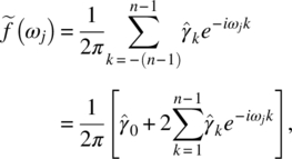
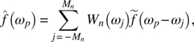
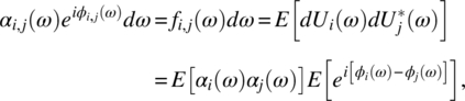
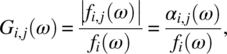
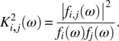
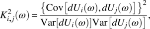
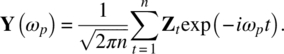
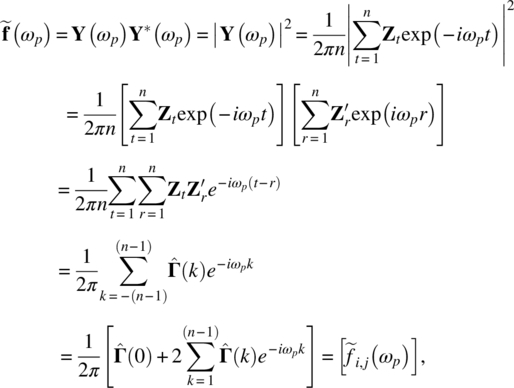
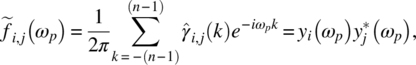
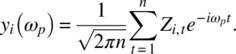
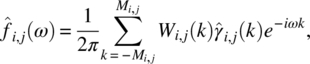
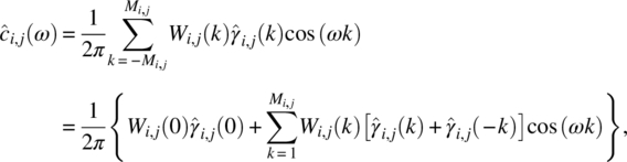
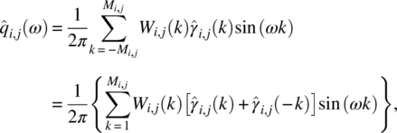
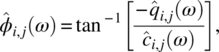
 , it implies that the range of the frequencies is from −π to π. Given a time series of length n, due to symmetry, the Fourier frequencies used in the sample spectrum will be ωj = 2πj/n, with j = 0, 1, …, [n/2]. However, if one writes the spectral density as
  it implies that the range of the frequencies will be −1/2 to 1/2. In this case, the frequencies used in the sample spectrum will be ωj = j/n, with j = 0, 1, …, [n/2]. In the following discussions, we may use either one depending on what is used in software and the referenced papers.

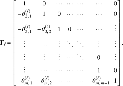
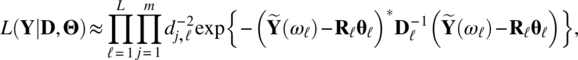
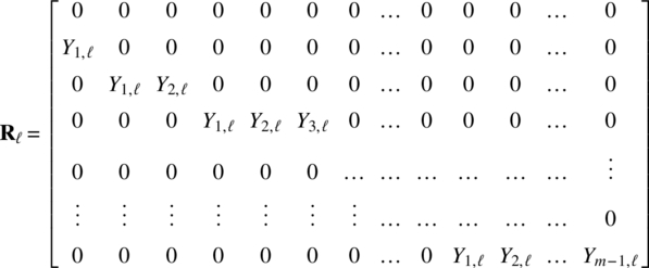
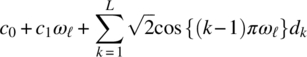
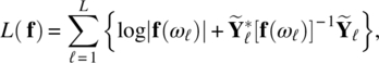
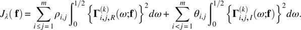
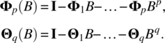
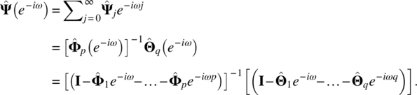

 ,
,  ,
,  , and
, and  ; estimated quadrature spectra (e–h):

 and
and  .
.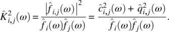
 ,
,  ,
,  ,
,  and estimated quadrature spectra (e–h):
  ,
,  ,
,  , and
, and  from the VAR(4) model.