5
Factor analysis of multivariate time series
Similar to principle component analysis, factor analysis is one of the commonly used dimension reduction methods. It is a statistical technique widely used to explain a m‐dimensional vector with a few underlying factors. After introducing different methods to derive factors, we will illustrate the method with empirical examples. We will also discuss its use in forecasting.
5.1 Introduction
Just like principle component analysis, the purpose of factor analysis is to approximate the covariance relationships among a set of variables. Specifically, it is used to describe the covariance relationships for many variables in terms of a relatively few underlying factors, which are unobservable random quantities. The concept was developed by the researchers in the field of psychometrics in the early twentieth century. It has become a commonly used statistical method in many areas.
5.2 The orthogonal factor model
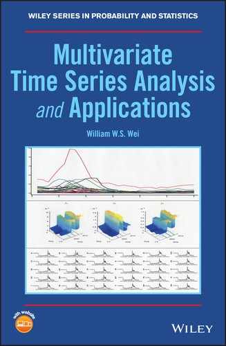
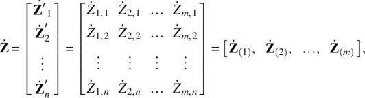
Given a weakly stationary m‐dimensional random vector at time t, Zt = [Z1,t, Z2,t, …, Zm,t]′ with mean μ = (μ1, μ2, …, μm)′, and covariance matrix Γ, the factor model assumes that Zt is dependent on a small number of k unobservable factors, Fj,t, j = 1, 2, …, k, known as common factors, and m additional noises εi,t, i = 1, 2, …, m, also known as specific factors, that is
More compactly, we can write the system in following matrix form,
where ![]() is a (k × 1) vector of factors at time t, L = [ℓi,j] is a (m × k) loading matrix, with ℓi,j is the loading of the ith variable on the jth factor, i = 1, 2, …, m, j = 1, 2, …, k, and εt = (ε1,t, ε2,t, …, εm,t)′ is a (m × 1) vector of noises, with E(εt) = 0, and
is a (k × 1) vector of factors at time t, L = [ℓi,j] is a (m × k) loading matrix, with ℓi,j is the loading of the ith variable on the jth factor, i = 1, 2, …, m, j = 1, 2, …, k, and εt = (ε1,t, ε2,t, …, εm,t)′ is a (m × 1) vector of noises, with E(εt) = 0, and ![]()
The factor model in Eq. (5.2) is an orthogonal factor model if it satisfies the following assumptions:
- E(Ft) = 0, and Cov(Ft) = Ik, the (k × k) identity matrix,
- E(εt) = 0, and
 a (m × m) diagonal matrix, and
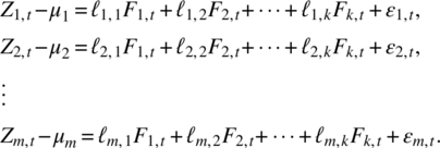
 - Ft and εt are independent and so
 a (k × m) zero matrix.
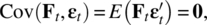
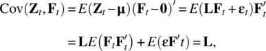
It follows from Eq. (5.2) that the covariance structure of Zt is
The model in Eq. (5.2) shows that the m‐dimensional process Zt is linear related to the k common factors. More specifically,
which implies that
Also,
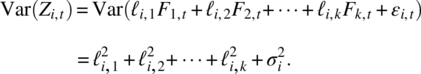
So the variance of the ith variable Zi,t is the sum ![]() due to the k common factors, which is known as the ith communality, and
due to the k common factors, which is known as the ith communality, and ![]() due to the ith specific factor, which is known as the ith specific variance.
due to the ith specific factor, which is known as the ith specific variance.
5.3 Estimation of the factor model
5.3.1 The principal component method
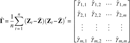
Given observations Zt = (Z1,t, Z2,t, …, Zm,t)′, for t = 1, 2, …, n, and its m × m sample covariance matrix ![]() a natural method of estimation is simply to use the principle component analysis introduced in Chapter 4 and choose k, which is much less than m, common factors from the first k largest eigenvalue‐eigenvector pairs in
a natural method of estimation is simply to use the principle component analysis introduced in Chapter 4 and choose k, which is much less than m, common factors from the first k largest eigenvalue‐eigenvector pairs in ![]() with
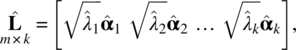
with ![]() Let
Let ![]() be the estimate of L. Then,
be the estimate of L. Then,
and the estimated specific variances are obtained by
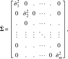
with the ith specific variance estimate being
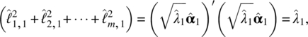
where the sum of squares is the estimate of the ith communality
The contribution to the first common factor to the total sample variance is given by
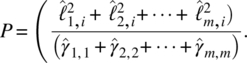
where we note that the eigenvectors in the principle component analysis are standardized to the unit length. More general, if we let P be the proportion of the jth common factor to the total sample variance, we have
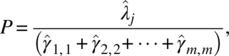
and it can be used to determine the desired number of common factors.
In practice, it is important to check carefully whether the units used in the component variables Zi,t, i = 1, 2, …, m, are comparable. If not, to avoid improperly influence of the units, we can standardize these variables, that is
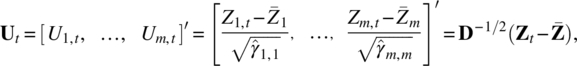
where D is the diagonal matrix in which the ith diagonal element is the sample variance of Zi,t, that is
Then, we will perform the principle component estimation method to the sample covariance matrix ![]() of the standardized observations Ut, t = 1,2, …, n, which is actually the sample correlation matrix of the original variables in Zt, t = 1,2, …, n.
of the standardized observations Ut, t = 1,2, …, n, which is actually the sample correlation matrix of the original variables in Zt, t = 1,2, …, n.
Again, the results from the sample covariance matrix and sample correlation matrix may not be the same, and the choice depends on applications.
5.3.2 Empirical Example 1 – Model 1 on daily stock returns from the second set of 10 stocks
5.3.3 The maximum likelihood method
When the common factors Ft and the specific factors εt can be assumed to be normally distributed, then Zt, t = 1, 2, …, n, will follow a multivariate normal distribution N(μ, Γ), and we can apply the maximum likelihood method to its likelihood function,
which is actually a function of L and Γ through the relationship Γ = LL′ + Σ, and μ is estimated by the sample mean ![]() However, because of Γ = LL′ + Σ = LΦΦ′L′ + Σ, and
However, because of Γ = LL′ + Σ = LΦΦ′L′ + Σ, and ![]() for any k × k orthogonal matrix Φ, to make Eq. (5.15) well defined, we also impose the following unique condition,
for any k × k orthogonal matrix Φ, to make Eq. (5.15) well defined, we also impose the following unique condition,
The maximum likelihood estimates ![]() and
and ![]() can be accomplished with numerical methods using statistical software such as EViews, MATLAB, MINITAB, R, SAS, and SPSS. However, the useful patterns of the factor loadings from the maximum likelihood solution obtained under the imposed unique condition may not be clear until the factors are rotated, which will be discussed later.
can be accomplished with numerical methods using statistical software such as EViews, MATLAB, MINITAB, R, SAS, and SPSS. However, the useful patterns of the factor loadings from the maximum likelihood solution obtained under the imposed unique condition may not be clear until the factors are rotated, which will be discussed later.
The maximum likelihood estimate of the ith communality is
and the proportion of the contribution of the ith common factor is by
To build a k common factor model for an m‐dimensional process, under the normal assumption, we can test the adequacy of the model with the following null hypothesis,
versus
To test the null hypothesis, we apply the likelihood ratio test
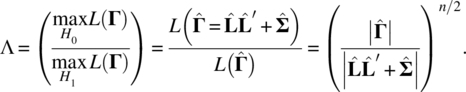
It is well known that

follows approximately the chi‐square distribution with degrees of freedom,
where we note that
is the MLE of Γ without any restriction, which has [(m2 + m)/2] free parameters, and
is the MLE of Γ under the restriction of factor model, which has (mk + m) parameters but with [(k2 − k)/2] constraints on the unique condition on ![]() being a k × k diagonal matrix given in Eq. (5.16). In practice, the test statistic in Eq. (5.22) will be replaced by Bartlett‐Corrected Test Statistic,
being a k × k diagonal matrix given in Eq. (5.16). In practice, the test statistic in Eq. (5.22) will be replaced by Bartlett‐Corrected Test Statistic,
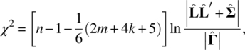
which gives a better approximation to the chi‐square distribution as shown by Bartlett (1954). Hence, the null hypothesis will be rejected if
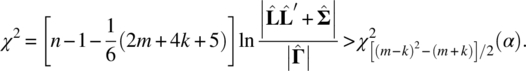
Because the degrees of freedom must be positive, we also require that
When correlation matrix ρ is used for factor analysis, the test statistic in Eq. (5.26) becomes
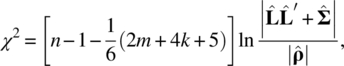
with exactly the same degrees of freedom, ![]() The reason is that the elements and computation of ρ are based on the covariance matrix Γ. The number of its free parameters is exactly the same as that of Γ. In terms of the m‐dimensional case, it is (m2 + m)/2.
The reason is that the elements and computation of ρ are based on the covariance matrix Γ. The number of its free parameters is exactly the same as that of Γ. In terms of the m‐dimensional case, it is (m2 + m)/2.
5.3.4 Empirical Example II – Model 2 on daily stock returns from the second set of 10 stocks
5.4 Factor rotation
It should be noted that regardless of what method is used in factor analysis, from Eq. (5.2), for any k × k orthogonal matrix Φ, we have
where
As a result, there are many multiple choices for L through orthogonal transformations, each of which is equivalent to rotating the common factors in the m‐dimensional space. This leads researchers to use arithmetic to find a new set of factor loadings so that the resulting common factors have easier and nicer interpretations. The methods are commonly known as factor rotations.
5.4.1 Orthogonal rotation
Let Ft* be the rotated factor and ![]() be the rotated matrix of factor loadings. One of the most widely used orthogonal rotation methods is the varimax proposed by Kaiser (1958), which finds an orthogonal transformation to maximize the sum of the variances of the squared loadings:
be the rotated matrix of factor loadings. One of the most widely used orthogonal rotation methods is the varimax proposed by Kaiser (1958), which finds an orthogonal transformation to maximize the sum of the variances of the squared loadings:
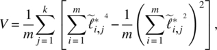
where

are the rotated coefficients scaled by the square root of communalities. The varimax will be achieved if any given variable has a high loading on a single factor but nearly zero loadings on the remaining factors or any given factor is formed by only a few variables with very high loadings and the remaining variables have nearly zero loadings on this factor. This is a widely used method for orthogonal rotation with all factors remaining uncorrelated. After the orthogonal transformation is determined, we will multiply the loadings ![]() by
by ![]() so that the original communalities are preserved.
so that the original communalities are preserved.
5.4.2 Oblique rotation
The orthogonal rotation methods like varimax assume that the factors in the analysis are independent. On the other hand, some researchers believe that the purpose of factor rotations is to achieve a simple structure with a new set of factor loadings so that the resulting common factors have simpler and nicer interpretations, and hence one should relax the independence assumption for the factors. The resulting method is often known as oblique rotation. Just like orthogonal rotations, there are many different forms of oblique rotation, see Carroll (1953, 1957), and Jennrich and Sampson (1966).
Although we introduce the rotation concept here, they are used for principal components analysis (PCA) too. There are many factor rotations available and they are implemented in statistical software like EViews, MATLAB, MINITAB, R, SAS, and SPSS. We will not spend more time on the discussion of various factor rotations. Instead, we would like to point out that the rationale of factor rotations is to simplify the factor structure with easier interpretation, and Thurstone (1947) suggested the following criteria:
- Each variable should produce at least one zero loading on some factor.
- Each factor should have at least as many nearly zero loadings as there are factors.
- Each pair of factors should have variables with significant loadings on one and near zero loadings on the other.
- Each pair of factors should have a large proportion of zero loadings on both factors.
- Each pair of factors should have only a small number of large loadings. For more details, we refer readers to a good multivariate analysis textbook by Johnson and Wichern (2007) and some relevant statistical software manuals.
5.4.3 Empirical Example III – Model 3 on daily stock returns from the second set of 10 stocks
5.5 Factor scores
5.5.1 Introduction
Once factor analysis is completed and parameters are estimated, we have ![]() and
and ![]() By treating these
By treating these ![]() and
and ![]() as known and their elements like the common factor loadings
as known and their elements like the common factor loadings ![]() and the variances
and the variances ![]() of specific factors as if they were the true values, we can estimate the values
of specific factors as if they were the true values, we can estimate the values ![]() of the unobserved random factor vector Ft, known as factor scores, from the Eq. (5.2), which repeats as follows:
of the unobserved random factor vector Ft, known as factor scores, from the Eq. (5.2), which repeats as follows:
where we regard the specific factors ![]() as errors. Because the variances
as errors. Because the variances ![]() of εi, t for i = 1, 2, …, m, can be unequal, Bartlett (1937) has suggested using the weighted least squares to estimate the common factor values, that is choosing the estimate
of εi, t for i = 1, 2, …, m, can be unequal, Bartlett (1937) has suggested using the weighted least squares to estimate the common factor values, that is choosing the estimate ![]() to minimize the following weighted sum of squares of the errors,
to minimize the following weighted sum of squares of the errors,
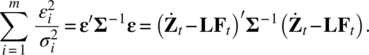
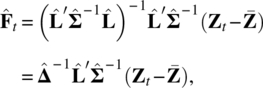
The solution from Chapter 3 can be easily seen to be
Thus, treating ![]() and
and ![]() as the true values, the factor scores for time t is obtained as
as the true values, the factor scores for time t is obtained as
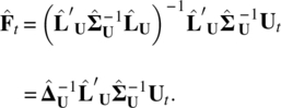
When the factor model is obtained through the standardized variables, ![]() that is through the correlation matrix, it becomes
that is through the correlation matrix, it becomes
When ![]() and
and ![]() are determined by the MLE, we have
are determined by the MLE, we have
where ![]() from Eq. (5.16). If the factor model is obtained through the standardized variables, then
from Eq. (5.16). If the factor model is obtained through the standardized variables, then
5.5.2 Empirical Example IV – Model 4 on daily stock returns from the second set of 10 stocks
5.6 Factor models with observable factors
In many applications, we can consider a factor model, where the factors Ft are observable with factor scores. For example, in some economic and financial studies, a commonly used factor model is the one where some macroeconomic variables and market indices such as inflation rate, industrial production index, employment and unemployment rates, interest rate, S&P 500 Index, Dow Jones Industrial Average (DJIA), and Consumer Price Index (CPI) can be used as factors, and they are observable.
When factors are observable, the factor loadings can be estimated using both Zt and Ft. Specifically, let ![]() we can rewrite the model in Eqs. (5.2) or (5.38) as
we can rewrite the model in Eqs. (5.2) or (5.38) as
Thus, for t = 1, 2, …, n, the whole system of the factor model can be expressed as the multivariate multiple time series regression,
where
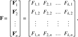
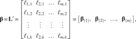
and
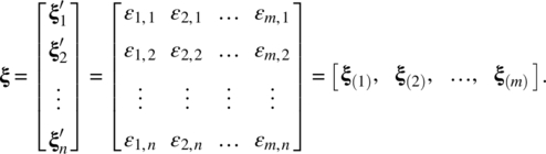
Each ξ(i) follows a n‐dimensional multivariate normal distribution ![]() i = 1, …, m, and ξ(i) and ξ(j) are uncorrelated if i ≠ j.
i = 1, …, m, and ξ(i) and ξ(j) are uncorrelated if i ≠ j.
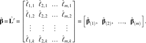
Equation (5.47) implies that
which is the standard matrix form of the multiple regression model, and the least squares estimate of β(i) is given by
Hence,
The residuals of Eq. (5.47) are
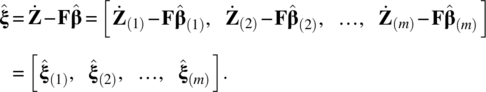
Under the assumption given in Eq. (5.2), the estimate of the covariance matrix of εt is
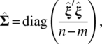
where diag(A) represents the diagonal matrix consisting of the diagonal elements of the matrix A.
In time series applications, given a m‐dimensional time series, ![]() it is natural to build a factor model with lag operator and a time series model on the factors as shown in the following,
it is natural to build a factor model with lag operator and a time series model on the factors as shown in the following,
or equivalently,
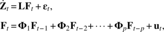
where all time series are assumed to be stationary, ut is a k‐dimensional zero mean white noise process independent of εt. The model is known as the dynamic factor model. It was first introduced by Geweke (1977) and has been widely used in practice. Once values of factors are obtained, we can combine the lagged values of Zt or other observed variables in the model and build a model for the h‐step ahead forecast for Zt + h,, that is
where Xt is a m × 1 vector of lagged values of Zt and/or other observed variables.
5.7 Another empirical example – Yearly U.S. sexually transmitted diseases (STD)
We will now consider a data set that contains yearly STD morbidity rates reported to National Center for HIV/AIDS, viral Hepatitis, STD, and TB Prevention (NCHHSTP), Center for HIV, and Centers for Disease Control and Prevention (CDC) from 1984 to 2013. The dataset was retrieved from CDC's website and includes 50 states plus D.C. The rates per 100000 persons are calculated as the incidence of STD reports, divided by the population, and multiple by 100000.
For the analysis, we remove data from following states, Montana, North Dakota, South Dakota, Vermont, Wyoming, Alaska, and Hawaii, due to missing data. Hence, the dimension of series Xt is m = 44 and n = 30. The data set is known as WW8c in the Data Appendix, and its plot is shown in Figure 5.3.
Figure 5.3 U.S. yearly STD of 43 states and D.C.
We first take difference of the series by Zt = (1 − B)Xt, and the differenced data are plotted in Figure 5.4. The analysis will be based on differenced data. We used the first 24 data points for model fitting, and the rest of observations for evaluating the forecasting performance.
Figure 5.4 The differenced yearly STD of 43 states and D.C.
5.7.1 Principal components analysis (PCA)
As discussed in Chapter 4, PCA can be based on a covariance matrix or a correlation matrix. For a high dimensional case, the print out of a covariance or correlation matrix is tedious. Since the correlation matrix is simply the covariance matrix of standardized variables, instead of saying that PCA is based on a covariance matrix or a correlation matrix, we will simply specify whether PCA is based on unstandardized variables or standardized variables.
5.7.1.1 PCA for standardized Zt
We first do PCA for Zt where the data set is standardized. The screeplot in Figure 5.5 shows that first six principal components can explain most of the variance so that first six components will be enough.
Figure 5.5 The screeplot for standardized variables.
The first six components from sample PCA for the standardized variables is given in Table 5.6.
Table 5.6 Sample PCA result for standardized variables.
| Comp. 1 |
Comp. 2 |
Comp. 3 |
Comp. 4 |
Comp. 5 |
Comp. 6 |
|
| CT | −0.127 | −0.215 | 0.200 | −0.046 | −0.193 | 0.191 |
| ME | 0.008 | 0.051 | −0.048 | −0.188 | −0.123 | 0.213 |
| MA | −0.196 | −0.176 | −0.071 | −0.144 | 0.063 | −0.064 |
| NH | −0.082 | 0.023 | −0.058 | 0.095 | −0.329 | −0.223 |
| RI | −0.141 | 0.055 | 0.212 | 0.138 | 0.081 | 0.230 |
| NJ | −0.214 | −0.155 | 0.026 | −0.216 | 0.020 | 0.089 |
| NY | −0.233 | −0.168 | −0.033 | 0.074 | −0.076 | −0.015 |
| DE | −0.137 | −0.031 | 0.217 | 0.067 | −0.336 | −0.070 |
| DC | −0.250 | −0.131 | −0.007 | 0.014 | 0.039 | −0.155 |
| MD | −0.170 | −0.168 | −0.011 | −0.068 | 0.208 | −0.134 |
| PA | −0.223 | −0.127 | 0.075 | −0.138 | −0.201 | 0.004 |
| VA | −0.213 | 0.021 | 0.009 | 0.113 | 0.204 | 0.254 |
| WV | −0.099 | 0.086 | 0.229 | 0.234 | 0.013 | 0.315 |
| AL | −0.237 | −0.042 | 0.060 | −0.083 | 0.204 | −0.025 |
| FL | 0 | −0.283 | −0.077 | 0.152 | −0.251 | 0.134 |
| GA | −0.208 | −0.183 | 0.122 | −0.027 | −0.101 | 0.044 |
| KY | −0.049 | 0.124 | −0.264 | −0.106 | −0.081 | 0.229 |
| MS | −0.096 | 0.179 | −0.174 | −0.128 | −0.061 | 0.101 |
| NC | −0.170 | 0.135 | −0.049 | 0.076 | −0.166 | −0.196 |
| SC | −0.203 | 0.113 | 0.043 | 0.228 | 0.162 | −0.006 |
| TN | −0.223 | −0.096 | −0.022 | −0.255 | 0.012 | 0.004 |
| IL | −0.212 | 0.178 | 0.007 | 0.105 | 0.003 | −0.149 |
| IN | −0.031 | 0.206 | −0.171 | −0.090 | −0.208 | 0.021 |
| MI | −0.245 | 0.010 | 0.054 | 0.115 | 0.141 | −0.075 |
| MN | −0.119 | 0.070 | −0.110 | 0.008 | −0.213 | 0.063 |
| OH | −0.111 | 0.217 | −0.217 | −0.115 | −0.058 | 0.143 |
| WI | −0.199 | 0.160 | −0.089 | 0.025 | 0.089 | 0.045 |
| AR | −0.199 | 0.164 | −0.003 | 0.144 | 0.006 | −0.194 |
| LA | −0.227 | 0.142 | −0.121 | −0.053 | 0.015 | 0.040 |
| NM | 0.029 | −0.127 | −0.292 | 0.110 | 0.160 | −0.001 |
| OK | −0.101 | 0.071 | −0.178 | −0.009 | −0.179 | −0.331 |
| TX | −0.232 | −0.031 | −0.072 | −0.063 | 0.190 | 0.069 |
| IA | −0.098 | 0.056 | −0.176 | 0.006 | 0.074 | 0.222 |
| KS | −0.129 | 0.175 | 0.087 | 0.308 | −0.054 | −0.125 |
| MO | −0.061 | 0.236 | −0.227 | −0.009 | −0.198 | 0.064 |
| NE | −0.053 | 0.070 | 0.154 | 0.242 | −0.100 | 0.178 |
| CO | 0.017 | 0.034 | −0.289 | 0.070 | 0.111 | 0.212 |
| UT | 0.007 | −0.063 | −0.185 | 0.283 | 0.067 | 0.086 |
| AZ | −0.073 | −0.227 | −0.174 | −0.187 | 0.089 | −0.165 |
| CA | −0.003 | −0.245 | −0.219 | 0.178 | −0.162 | 0.043 |
| NV | 0.001 | −0.190 | −0.225 | 0.099 | 0.047 | 0.025 |
| ID | 0.018 | −0.129 | −0.17 | 0.276 | 0.153 | −0.168 |
| OR | 0.045 | −0.202 | −0.203 | 0.327 | −0.079 | 0.009 |
| WA | −0.053 | −0.256 | −0.043 | 0.041 | −0.221 | 0.226 |
| Variance |
12.128 | 7.218 | 5.228 | 3.478 | 3.192 | 2.561 |
| Cumulative Percentage | 27.56 | 43.97 | 55.85 | 63.76 | 71.01 | 76.83 |
Let us look at the plot for the first and second components of these time series in Figure 5.6.
Figure 5.6 The first and second components for standardized variables.
It appears that states that are spatially close are also tending to be close to each other in the component plot. For examples: (i) NJ, NY, PA, DC; (ii) OH, KS, MS, MO; and (iii) CA, OR, NV, WA.
5.7.1.2 PCA for unstandardized Zt
Now, let us look at what the result is when we apply PCA on unstandardized Zt, which is equivalent to the construction of the PCA model based on the covariance matrix of Zt. The screeplot in Figure 5.7 shows that first three principal components can explain most of the variance, so we will choose a three‐component PCA model.
Figure 5.7 The screeplot for unstandardized variables.
The first three components from a sample PCA for the unstandardized variables are given in Table 5.7.
Table 5.7 Sample PCA result for unstandardized variables.
| Comp. 1 |
Comp. 2 |
Comp. 3 |
|
| CT | 0.064 | 0.115 | −0.016 |
| ME | −0.002 | −0.004 | −0.001 |
| MA | 0.042 | 0.018 | 0.001 |
| NH | 0.005 | −0.001 | −0.004 |
| RI | 0.018 | −0.026 | 0.054 |
| NJ | 0.067 | 0.007 | −0.018 |
| NY | 0.138 | 0.028 | −0.133 |
| DE | 0.073 | 0.025 | 0.079 |
| DC | 0.900 | 0.098 | 0.098 |
| MD | 0.097 | 0.058 | 0.059 |
| PA | 0.093 | 0.011 | −0.024 |
| VA | 0.040 | −0.043 | −0.003 |
| WV | 0.007 | −0.013 | 0.051 |
| AL | 0.117 | −0.061 | 0.115 |
| FL | 0.054 | 0.396 | −0.482 |
| GA | 0.188 | 0.115 | −0.038 |
| KY | 0 | −0.029 | −0.045 |
| MS | 0.034 | −0.597 | −0.560 |
| NC | 0.057 | −0.116 | −0.029 |
| SC | 0.081 | −0.131 | 0.110 |
| TN | 0.113 | −0.041 | −0.052 |
| IL | 0.058 | −0.137 | 0.056 |
| IN | −0.004 | −0.047 | −0.030 |
| MI | 0.059 | −0.035 | 0.053 |
| MN | 0.006 | −0.013 | −0.012 |
| OH | 0.007 | −0.091 | −0.057 |
| WI | 0.024 | −0.062 | 0.011 |
| AR | 0.091 | −0.206 | 0.050 |
| LA | 0.182 | −0.451 | −0.094 |
| NM | 0.003 | 0.045 | −0.135 |
| OK | 0.017 | −0.038 | −0.026 |
| TX | 0.079 | −0.057 | −0.030 |
| IA | 0.003 | −0.017 | −0.025 |
| KS | 0.012 | −0.027 | 0.047 |
| MO | −0.001 | −0.146 | −0.120 |
| NE | 0 | −0.001 | 0.006 |
| CO | −0.004 | −0.010 | −0.042 |
| UT | 0.001 | 0.010 | −0.019 |
| AZ | 0.040 | 0.055 | −0.069 |
| CA | 0.025 | 0.137 | −0.239 |
| NV | 0.046 | 0.254 | −0.487 |
| ID | 0.004 | 0.019 | −0.015 |
| OR | 0.003 | 0.090 | −0.124 |
| WA | 0.011 | 0.039 | −0.052 |
| Variance |
3472.528 | 717.536 | 332.014 |
| Cumulative Percentage | 65.55 | 79.10 | 85.37 |
As shown in Figure 5.8, the plot of the first and second components for the unstandardized variables is very different from the one for standardized variables. It suggests that the unstandardized data does not produce similar or good separation as the standardized data does. It also shows that PCA for standardized variables is much more robust. So, we will use standardized variables for our PCA model.
Figure 5.8 The first and second components for unstandardized variables.
5.7.2 Factor analysis
To build a factor model, we can either use the principle components method or maximum likelihood estimation method. However, for our data set, we have a vector series with a dimension m = 44 and n = 30. Its maximum likelihood equation cannot be properly solved. So, we can only use the principle component method. Thus, we will use PCA to estimate factors. In this analysis, we will follow Bai and Ng (2002), and select six factors, which is supported by the screeplot shown in Figure 5.5.
From the PCA analysis in Section 5.7.1, we will choose a factor model with six common factors,
based on the standardized variables. The corresponding factor loadings, communalities, and specific variables are given in Table 5.8. The six estimated factor scores are plotted in Figure 5.9.
Table 5.8 The principal component estimation for the factor model from the STD data set.
| CT | −0.442 | −0.577 | 0.456 | −0.086 | −0.344 | 0.306 | 0.956 | 0.044 |
| ME | 0.029 | 0.136 | −0.110 | −0.350 | −0.219 | 0.341 | 0.319 | 0.681 |
| MA | −0.683 | −0.473 | −0.163 | −0.269 | 0.113 | −0.102 | 0.812 | 0.188 |
| NH | −0.285 | 0.063 | −0.133 | 0.178 | −0.588 | −0.357 | 0.607 | 0.393 |
| RI | −0.492 | 0.149 | 0.485 | 0.257 | 0.145 | 0.368 | 0.722 | 0.278 |
| NJ | −0.747 | −0.417 | 0.059 | −0.403 | 0.036 | 0.143 | 0.919 | 0.081 |
| NY | −0.813 | −0.451 | −0.075 | 0.137 | −0.136 | −0.024 | 0.907 | 0.093 |
| DE | −0.479 | −0.082 | 0.495 | 0.124 | −0.601 | −0.113 | 0.870 | 0.130 |
| DC | −0.869 | −0.352 | −0.015 | 0.026 | 0.070 | −0.248 | 0.948 | 0.052 |
| MD | −0.592 | −0.452 | −0.025 | −0.128 | 0.372 | −0.214 | 0.756 | 0.244 |
| PA | −0.778 | −0.342 | 0.172 | −0.258 | −0.359 | 0.007 | 0.947 | 0.053 |
| VA | −0.743 | 0.055 | 0.021 | 0.211 | 0.365 | 0.407 | 0.900 | 0.100 |
| WV | −0.345 | 0.231 | 0.525 | 0.436 | 0.022 | 0.503 | 0.892 | 0.108 |
| AL | −0.825 | −0.112 | 0.137 | −0.155 | 0.364 | −0.039 | 0.870 | 0.130 |
| FL | −0.002 | −0.761 | −0.176 | 0.284 | −0.449 | 0.215 | 0.938 | 0.062 |
| GA | −0.723 | −0.491 | 0.279 | −0.050 | −0.180 | 0.070 | 0.883 | 0.117 |
| KY | −0.172 | 0.332 | −0.602 | −0.197 | −0.144 | 0.366 | 0.697 | 0.303 |
| MS | −0.336 | 0.482 | −0.398 | −0.239 | −0.110 | 0.161 | 0.599 | 0.401 |
| NC | −0.591 | 0.363 | −0.111 | 0.142 | −0.297 | −0.314 | 0.701 | 0.299 |
| SC | −0.709 | 0.304 | 0.098 | 0.425 | 0.289 | −0.010 | 0.868 | 0.132 |
| TN | −0.778 | −0.258 | −0.050 | −0.475 | 0.022 | 0.006 | 0.900 | 0.100 |
| IL | −0.737 | 0.479 | 0.017 | 0.196 | 0.006 | −0.238 | 0.869 | 0.131 |
| IN | −0.108 | 0.553 | −0.391 | −0.168 | −0.372 | 0.033 | 0.637 | 0.363 |
| MI | −0.852 | 0.026 | 0.124 | 0.214 | 0.252 | −0.120 | 0.866 | 0.134 |
| MN | −0.415 | 0.187 | −0.253 | 0.016 | −0.381 | 0.101 | 0.426 | 0.574 |
| OH | −0.385 | 0.584 | −0.495 | −0.215 | −0.104 | 0.230 | 0.844 | 0.156 |
| WI | −0.694 | 0.429 | −0.202 | 0.046 | 0.159 | 0.072 | 0.739 | 0.261 |
| AR | −0.693 | 0.441 | −0.006 | 0.268 | 0.011 | −0.311 | 0.843 | 0.157 |
| LA | −0.791 | 0.380 | −0.276 | −0.099 | 0.027 | 0.065 | 0.862 | 0.138 |
| NM | 0.100 | −0.342 | −0.669 | 0.204 | 0.286 | −0.002 | 0.697 | 0.303 |
| OK | −0.350 | 0.190 | −0.408 | −0.017 | −0.320 | −0.530 | 0.709 | 0.291 |
| TX | −0.808 | −0.083 | −0.164 | −0.118 | 0.340 | 0.110 | 0.829 | 0.171 |
| IA | −0.343 | 0.150 | −0.402 | 0.012 | 0.132 | 0.356 | 0.446 | 0.554 |
| KS | −0.451 | 0.470 | 0.199 | 0.574 | −0.096 | −0.200 | 0.843 | 0.157 |
| MO | −0.212 | 0.635 | −0.520 | −0.017 | −0.354 | 0.102 | 0.855 | 0.145 |
| NE | −0.186 | 0.187 | 0.352 | 0.451 | −0.179 | 0.285 | 0.510 | 0.490 |
| CO | 0.058 | 0.090 | −0.661 | 0.131 | 0.198 | 0.339 | 0.620 | 0.380 |
| UT | 0.026 | −0.170 | −0.424 | 0.528 | 0.119 | 0.137 | 0.521 | 0.479 |
| AZ | −0.253 | −0.609 | −0.397 | −0.349 | 0.158 | −0.264 | 0.810 | 0.190 |
| CA | −0.010 | −0.658 | −0.501 | 0.331 | −0.289 | 0.069 | 0.882 | 0.118 |
| NV | 0.003 | −0.511 | −0.514 | 0.184 | 0.085 | 0.040 | 0.568 | 0.432 |
| ID | 0.064 | −0.347 | −0.389 | 0.514 | 0.274 | −0.269 | 0.687 | 0.313 |
| OR | 0.157 | −0.543 | −0.464 | 0.609 | −0.140 | 0.014 | 0.926 | 0.074 |
| WA | −0.186 | −0.687 | −0.097 | 0.076 | −0.396 | 0.362 | 0.809 | 0.191 |
Figure 5.9 The estimated six common factor scores for the STD data set.
So, we have our factor model for the STD data set,
where the element and specification of L, Ft, and εt are given in Table 5.8. As described in Section 5.6, once values or scores of factors are estimated, we can combine the lagged values of Zt or other observed variables in the model and build a forecast equation for the h‐step ahead forecast for Zt + h,, that is
where Vt are lagged values of Zt and/or other observed variables, and ![]() and
and ![]() are the parameter estimates based on Vt given in Eq. (5.57).
are the parameter estimates based on Vt given in Eq. (5.57).
In this example, we will simply choose Vt to be the first lagged value of Zt. Specifically, our forecasting equations will be
where ![]() is the ith row of
is the ith row of ![]() and
and ![]() is the ith element of
is the ith element of ![]() For i = 1, we have
For i = 1, we have
and for h = 1, it becomes
From the estimation results, we have
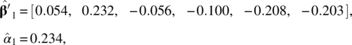
and the factor scores, ![]() for t = 1, 2, …, 24, and Z1, t are given in Table 5.9.
for t = 1, 2, …, 24, and Z1, t are given in Table 5.9.
Table 5.9 The estimated factor scores and standardized Z1,t.
| t | Factor 1 | Factor 2 | Factor 3 | Factor 4 | Factor 5 | Factor 6 | t | Z1,t |
| 1 | 0.754 | 0.729 | 0.745 | 0.872 | −1.280 | 0.629 | 1 | 0.147 |
| 2 | 1 | 0.745 | 0.338 | −0.181 | 1.160 | −0.686 | 2 | 0.010 |
| 3 | −1.165 | 6.198 | −2.948 | −2.638 | 3.382 | 0.107 | 3 | 1.067 |
| 4 | −4.217 | 3.103 | −0.599 | −0.511 | 1.237 | −2.825 | 4 | 2.033 |
| 5 | −7.161 | −1.663 | 7.076 | 3.145 | 0.621 | −1.730 | 5 | 3.342 |
| 6 | −9.685 | −0.185 | −4.299 | 1.901 | −3.252 | 3.630 | 6 | −0.734 |
| 7 | −2.813 | −7.658 | 0.829 | −6.294 | −0.704 | 0.553 | 7 | −2.073 |
| 8 | 3.543 | −6.566 | −1.992 | 2.611 | 4.981 | 1.335 | 8 | −1.996 |
| 9 | 4.445 | −2.224 | −4.613 | 2.797 | −2.742 | −2.706 | 9 | −1.102 |
| 10 | 5.751 | −0.298 | 1.360 | −0.786 | −3.816 | −1.423 | 10 | −0.866 |
| 11 | 3.709 | 1.050 | 1.099 | 0.630 | 0.403 | 3.209 | 11 | −0.221 |
| 12 | 3.850 | 3.066 | 3.592 | −0.027 | −1.059 | 2.854 | 12 | 0.310 |
| 13 | 1.635 | 1.396 | 1.014 | −0.166 | −0.407 | 0.536 | 13 | 0.013 |
| 14 | 2.646 | 0.108 | 0.792 | −0.176 | 0.169 | 0.647 | 14 | −0.545 |
| 15 | 0.848 | −0.276 | −0.209 | 0.475 | 0.757 | 0.074 | 15 | −0.153 |
| 16 | 0.976 | 0.642 | 0.110 | −0.044 | −0.578 | −0.014 | 16 | 0.151 |
| 17 | −0.379 | 0.595 | 0.538 | 0.131 | −0.044 | −0.359 | 17 | 0.105 |
| 18 | 0.043 | 0.731 | −0.428 | −1.389 | −0.046 | −0.573 | 18 | 0.140 |
| 19 | −0.511 | 0.428 | −0.605 | −0.078 | 0.908 | −0.134 | 19 | 0.124 |
| 20 | 0.371 | 0.566 | −0.164 | −1.795 | −0.571 | −0.642 | 20 | −0.096 |
| 21 | −0.046 | −0.380 | 0.455 | 0.857 | 0.764 | −0.215 | 21 | 0.043 |
| 22 | −1.106 | −0.071 | −0.497 | 0.511 | −0.117 | −1.552 | 22 | 0.175 |
| 23 | −1.171 | 0.221 | 0.035 | 0.340 | 0.145 | 0.600 | 23 | −0.133 |
| 24 | −1.317 | −0.255 | −1.629 | −0.185 | 0.089 | −1.316 | 24 | 0.151 |
Based on Z1,24 = 0.151 and ![]() the one‐step‐ahead forecasting of the first time series is
the one‐step‐ahead forecasting of the first time series is
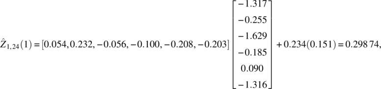
which is shown as the forecast for Connecticut in Table 5.10.
Table 5.10 The one‐step forecast result for the standardized STD series.
| State | Forecast | Actual | Error | State | Forecast | Actual | Error |
| CT | 0.299 | 0.075 | 0.224 | IN | 0.08 | −0.194 | 0.274 |
| ME | −0.488 | −0.922 | 0.434 | MI | 0.06 | 0.194 | −0.134 |
| MA | −0.313 | −0.088 | −0.225 | MN | 0.042 | −0.875 | 0.917 |
| NH | 0.375 | −0.465 | 0.84 | OH | 0.392 | 0.042 | 0.35 |
| RI | 0.8 | 0.297 | 0.503 | WI | 0.333 | −0.143 | 0.476 |
| NJ | 0.198 | −0.168 | 0.366 | AR | 0.38 | 0.14 | 0.24 |
| NY | 0.281 | −0.456 | 0.737 | LA | 0.162 | −0.077 | 0.239 |
| DE | 0.233 | 0.283 | −0.05 | NM | 0.256 | 0.227 | 0.029 |
| DC | 0.08 | 0.213 | −0.133 | OK | −0.285 | 0.352 | −0.637 |
| MD | −0.254 | −0.217 | −0.037 | TX | 0.25 | 0.574 | −0.324 |
| PA | 0.198 | 0.127 | 0.071 | IA | 0.689 | −0.435 | 1.124 |
| VA | 0.587 | −0.067 | 0.654 | KS | −0.059 | 0.382 | −0.441 |
| WV | 0.339 | −0.046 | 0.385 | MO | −0.382 | −0.074 | −0.308 |
| AL | 0.067 | −0.066 | 0.133 | NE | 0.33 | 0.369 | −0.039 |
| FL | −0.03 | −0.161 | 0.131 | CO | −0.789 | −1.05 | 0.261 |
| GA | 0.332 | −0.047 | 0.379 | UT | −0.313 | 0.279 | −0.592 |
| KY | 0.046 | 0.219 | −0.173 | AZ | −0.381 | −0.952 | 0.571 |
| MS | 0.995 | 0.073 | 0.922 | CA | −0.525 | −0.276 | −0.249 |
| NC | 0.549 | 0.888 | −0.339 | NV | 0.771 | −0.053 | 0.824 |
| SC | 0.241 | 0.367 | −0.126 | ID | −0.095 | 0.225 | −0.32 |
| TN | 0.11 | 0.07 | 0.04 | OR | −0.058 | 0.173 | −0.231 |
| IL | 0.23 | 0.46 | −0.23 | WA | 0.052 | −0.893 | 0.945 |
The mean squared forecast error (MSFE) is 0.222. It should be noted that the series we have used in model fitting and forecasting are standardized differenced series of the original data set.
5.8 Concluding remarks
In time series applications, it is natural to consider the observable factors in terms of some time series structures and use time lag operator and time series models on the factors. As a result, many different forms of factor models have been developed. The use of time series models such as vector autoregressive models on factors has also been extended to vector time series modeling in both time domain and frequency domain approaches. Some good examples are the various dynamic factor models.
For further information on factor models and applications, we recommend to readers Sharpe (1970), Geweke (1977), Engle and Watson (1981), Geweke and Sinleton (1981), Harvey (1989), Bai and Ng (2002, 2007), Garcia‐Ferrer and Poncela 2002, Bai (2003), Peña and Poncela (2004), Deistler and Zinner (2007), Hallin and Liska (2007), Doz et al. (2011), Jungbacker et al. (2011), Stock and Watson (2009, 2011, 2016), Lam and Yao (2012), Fan et al. (2016), Rockova and George (2016), Chan et al. (2017), and Gonçalves et al. (2017), among others.
Projects
- Find a multivariate analysis book and carefully read its chapter on factor analysis.
- Find a m‐dimensional social science related time series data set with m ≥ 10, construct your best factor models based on both principle component and likelihood ratio test methods, and compare your results with a written report and analysis software code. Email your data set and software code to your course instructor.
- Let Zt be the m‐dimensional vector in Project 1. Build a forecast equation to compute three‐step ahead forecasts for
- Find a m‐dimensional natural science related time series data set with m ≥ 20, construct your best factor models based on both principle component and likelihood ratio test methods and compare your results with a written report and analysis software code. Email your data set and software code to your course instructor.
- Let Zt be the m‐dimensional vector in Project 4. Build a forecast equation to compute five‐step ahead forecasts for
References
- Bai, J. (2003). Inferential theory for factor models of large dimensions. Econometrica 71: 135–171.
- Bai, J. and Ng, S. (2002). Determining the number of factors in approximate factor models. Econometrica 70: 191–221.
- Bai, J. and Ng, S. (2007). Determining the number of primitive shocks in factor models. American Statistical Association. Journal of Business & Economic Statistics 25: 52–60.
- Bartlett, M.S. (1937). The statistical concept of mental factors. British Journal of Psychology 28: 97–104.
- Bartlett, M.S. (1954). A note on multiplying factors for various chi‐squared approximation. Journal of the Royal Statistical Society, Series B 16: 296–298.
- Carroll, J.B. (1953). An analytic solution for approximating simple structure in factor analysis. Psychometrika 18: 23–38.
- Carroll, J.B. (1957). Biquartimin criterion for rotation to oblique simple structure in factor analysis. Science 126: 1114–1115.
- Chan, N.H., Lu, Y., and Yau, C.Y. (2017). Factor modelling for high‐dimensional time series: inference and model selection. Journal of Time Series Analysis 38: 285–307.
- Deistler, M. and Zinner, C. (2007). Modelling high‐dimensional time series by generalized linear dynamic factor models; an introductory survey. Communications in Information and Systems 7: 153–166.
- Doz, C., Giannone, D., and Reichlin, L. (2011). A two‐step estimator for large approximate dynamic factor models based on Kalman filtering. Journal of Econometrics 164: 188–205.
- Engle, R.F. and Watson, M.W. (1981). A one‐factor multivariate time series model of metropolitan wage rates. Journal of American Statistical Association 76: 774–781.
- Fan, J., Liao, Y., and Wang, W. (2016). Projected principal component analysis in factor models. Annals of Statistics 44: 219–254.
- Garcia‐Ferrer, A. and Poncela, P. (2002). Forecasting international GNP data through common factor models and other procedures. Journal of Forecasting 21: 225–244.
- Geweke, J.F. (1977). The dynamic factor analysis of economic time series. In: Latent Variables in Socio‐Economic Models (ed. D.J. Aigner and A.S. Goldberger). North‐Holland, Amsterdam: Elsevier.
- Geweke, J.F. and Sinleton, K.J. (1981). Maximum likelihood confirmatory factor analysis of economic time series. International Economic Review 22: 37–54.
- Gonçalves, S., Perron, B., and Djogbenou, A. (2017). Bootstrap prediction intervals for factor models. Journal of Business & Economic Statistics 35: 53–69.
- Hallin, M. and Liska, R. (2007). The generalized dynamic factor model: determining the number of factors. Journal of American Statistical Association 102: 603–617.
- Harvey, A.C. (1989). Forecasting Structural Time Series Models and the Kalman Filter. Cambridge University Press.
- Jennrich, R.I. and Sampson, P.F. (1966). Rotation for simple loadings. Psychometrica 31: 313–323.
- Johnson, R.A. and Wichern, D.W. (2007). Applied Multivariate Statistical Analysis, 6e. Englewood Cliffs, NJ: Pearson Prentice Hall.
- Jungbacker, B., Koopman, S.J., and van der Wel, M. (2011). Maximum likelihood estimation for dynamic factor models with missing data. Journal of Economic Dynamics & Control 35: 1358–1368.
- Kaiser, H.F. (1958). The varimax criterion for analytic rotation in factor analysis. Psychometrika 23: 187–200.
- Lam, C. and Yao, Q. (2012). Factor modeling for high‐dimensional time series: inference for the number of factors. Annals of Statistics 40: 694–726.
- Peña, D. and Poncela, P. (2004). Forecasting with nonstationary dynamic factor model. Journal of Econometrics 119: 291–321.
- Rockova, V. and George, E. (2016). Fast Bayesian factor analysis via automatic rotations to sparsity. Journal of American Statistical Association 111: 1608–1622.
- Sharpe, W. (1970). Portfolio Theory and Capital Markets. New York: McGraw‐Hill.
- Stock, J.H. and Watson, M.W. (2009). Forecasting in dynamic factor models subject to structural instability, Chapter 7. In: The Methodology and Practice of Econometrics: Festschrift in Honor of D.F. Hendry (ed. N. Shephard and J. Castle). Oxford University Press.
- Stock, J.H. and Watson, M.W. (2011). Dynamic factor models. In: The Oxford Handbook on Economic Forecasting (ed. M.P. Clements and D.F. Hendry), 35–59. Oxford University Press.
- Stock, J.H. and Watson, M.W. (2016). Dynamic factor models, factor‐augmented vector autoregressions, and structural vector autoregressions in macroeconomics. Handbook of Macroeconomics, Elsevier 415–525.
- Thurstone, L.L. (1947). Multiple‐Factor Analysis. Chicago: University of Chicago Press.