
2
The Core Model
2.1 Bayesian Meta-Analysis
There is a substantial literature on statistical methods for meta-analysis, going back to methods for combination of results from two-by-two tables and the introduction of random effects meta-analysis (DerSimonian and Laird, 1986), an important benchmark in the development of the field. Over the years methodological and software advances have contributed to the widespread use of meta-analytic techniques. A series of instructional texts and reviews have appeared (Cooper and Hedges, 1994; Smith et al., 1995; Egger et al., 2001; Sutton and Abrams, 2001; Higgins and Green, 2008; Sutton and Higgins, 2008), but there have been only a few attempts to produce a comprehensive guide to the statistical theory behind meta-analysis (Whitehead and Whitehead, 1991; Whitehead, 2002).
We present a single unified framework for evidence synthesis of aggregate data from RCTs that delivers an internally consistent set of estimates while respecting the randomisation in the evidence (Glenny et al., 2005). The core models presented in this chapter can synthesise data from pairwise meta-analysis, indirect and mixed treatment comparisons, that is, network meta-analysis (NMA) with or without multi-arm trials (i.e. trials with more than two arms), without distinction. Indeed, pairwise meta-analysis and indirect comparisons are special cases of NMA, and the general NMA model and WinBUGS code presented here instantiate that.
We take a Bayesian approach to synthesis using Markov chain Monte Carlo (MCMC) implemented in WinBUGS (Lunn et al., 2013) mainly due to the flexibility of the Bayesian approach, ease of implementation of models and parameter estimation in WinBUGS and its natural extension to decision modelling (see Preface). While we do not describe Bayesian methods, MCMC or the basics of running WinBUGS in this book, basic knowledge of all these concepts is required to fully understand the code presented. However, the underlying principles and concepts described can still be understood without detailed knowledge of Bayesian methods, MCMC or WinBUGS. Further references and a guide on how to read the book are given in the Preface.
We begin by presenting the core Bayesian models for meta-analysis of aggregate data presented as the number of events observed in a fixed and known number of individuals – commonly referred to as binary, dichotomous or binomial data. We describe fixed and random treatment effects models and show how the core models, based on the model proposed by Smith et al. (1995) for pairwise meta-analysis, are immediately applicable to indirect comparisons and NMA with multi-arm trials without the need for any further extension. This general framework is then applied to other types of data in Chapter 4.
2.2 Development of the Core Models
Consider a set of M trials comparing two treatments, 1 and 2, in a pre-specified target patient population, which are to be synthesised in a meta-analysis. A fixed effects analysis would assume that each study i generates an estimate of the same parameter d12, the relative effect of treatment 2 compared with 1 on some scale, subject to sampling error. In a random effects model, each study i provides an estimate of the study-specific treatment effects δi,12, the relative effect of treatment 2 compared with 1 on some scale in trial i, which are assumed not to be equal but rather exchangeable. This means that all δi,12 are ‘similar’ in a way that assumes that the trial labels, i, attached to the treatment effects δi,12 are irrelevant. In other words, the information that the trials provide is independent of the order in which they were carried out, over the population of interest (Bernardo and Smith, 1994). The exchangeability assumption is equivalent to saying that the trial-specific treatment effects come from a common distribution, and this is often termed the ‘random effects distribution’. In a Bayesian framework, the study-specific treatment effects, δi, are estimated for each study and are often termed the ‘shrunken’ estimates. They estimate the ‘true’ treatment effect for each trial and therefore ‘shrink’ the observed trial effects towards the random effects mean. See Chapters 3 and 8 for further details. The normal distribution is often chosen, so that
with d12 and ![]() representing the mean and variance, respectively. However, as we will see, any other suitable distribution could be chosen instead, and this could be implemented in WinBUGS. Note that the mean of the random effects distribution is the pooled effect of treatment 2 compared with 1, which is the main parameter of interest in a meta-analysis. It follows that the fixed effects model is a special case, obtained by setting the variance to zero, implying that δi,12 = d12 for all i.
representing the mean and variance, respectively. However, as we will see, any other suitable distribution could be chosen instead, and this could be implemented in WinBUGS. Note that the mean of the random effects distribution is the pooled effect of treatment 2 compared with 1, which is the main parameter of interest in a meta-analysis. It follows that the fixed effects model is a special case, obtained by setting the variance to zero, implying that δi,12 = d12 for all i.
In a Bayesian framework the parameters to be estimated are given prior distributions. In general we will want the observed data from the RCTs to be the main, overwhelming, influence on the estimated treatment effects and will therefore consider non-informative or minimally informative prior distributions, wherever possible. The degree of information in a prior distribution is intimately related to the range of plausible values for a parameter. For the pooled treatment effect d12, we assume that it has been specified on a continuous scale and that it can take any value between plus and minus infinities (see Section 2.2.1). An appropriate (non-informative) prior distribution is then
where the variance is very large, meaning that the distribution is essentially flat over the plausible range of values for the treatment effect.
For the between-study heterogeneity variance ![]() , the chosen prior distribution must be constrained to give only positive values, and a reasonable upper bound will depend on the expected range of observed treatment effects. We will choose uniform prior distributions with lower bound at zero and a suitable upper bound for the outcome measure being considered. In Section 2.3.2 alternative prior distributions are discussed.
, the chosen prior distribution must be constrained to give only positive values, and a reasonable upper bound will depend on the expected range of observed treatment effects. We will choose uniform prior distributions with lower bound at zero and a suitable upper bound for the outcome measure being considered. In Section 2.3.2 alternative prior distributions are discussed.
2.2.1 Worked Example: Meta-Analysis of Binomial Data
Caldwell et al. (2005) extended the thrombolytics network presented in Chapter 1 by adding studies from another systematic review on the same patient population, which also included an extra treatment (Keeley et al., 2003b). This extended network is presented in Figure 2.1.
Figure 2.1 Extended thrombolytics example: network plot. Seven treatments are compared (data from Caldwell et al., 2005): Streptokinase (SK), tissue-plasminogen activator (t-PA), accelerated tissue-plasminogen activator (Acc t-PA), reteplase (r-PA), tenecteplase (TNK), percutaneous transluminal coronary angioplasty (PTCA). The numbers on the lines and line thickness represent the number of studies making those comparisons, the widths of the circles are proportional to the number of patients randomised to each treatment, and the numbers in brackets are the treatment codes used in WinBUGS.
The data available are the number of mortalities by day 35, out of the total number of patients in each arm of the 36 included trials (Table 2.1). We will start by specifying the fixed and random effects two-treatment (pairwise) meta-analysis models and WinBUGS code for PTCA compared with Acc t-PA and will then extend the models and code to incorporate all available treatments and trials.
Table 2.1 Extended thrombolytics example.
Data from Caldwell et al. (2005).
| Study ID | Year | Number of arms | Arm 1 | Arm 2 | Arm 3 | Arm 1 | Arm 2 | Arm 3 | |||
| Events | Patients | Events | Patients | Events | Patients | ||||||
| GUSTO-1 | 1993 | 3 | SK | Acc t-PA | SK + t-PA | 1,472 | 20,251 | 652 | 10,396 | 723 | 10,374 |
| ECSG | 1985 | 2 | SK | t-PA | 3 | 65 | 3 | 64 | |||
| TIMI-1 | 1987 | 2 | SK | t-PA | 12 | 159 | 7 | 157 | |||
| PAIMS | 1989 | 2 | SK | t-PA | 7 | 85 | 4 | 86 | |||
| White | 1989 | 2 | SK | t-PA | 10 | 135 | 5 | 135 | |||
| GISSI-2 | 1990 | 2 | SK | t-PA | 887 | 10,396 | 929 | 10,372 | |||
| Cherng | 1992 | 2 | SK | t-PA | 5 | 63 | 2 | 59 | |||
| ISIS-3 | 1992 | 2 | SK | t-PA | 1,455 | 13,780 | 1,418 | 13,746 | |||
| CI | 1993 | 2 | SK | t-PA | 9 | 130 | 6 | 123 | |||
| KAMIT | 1991 | 2 | SK | SK + t-PA | 4 | 107 | 6 | 109 | |||
| INJECT | 1995 | 2 | SK | r-PA | 285 | 3,004 | 270 | 3,006 | |||
| Zijlstra | 1993 | 2 | SK | PTCA | 11 | 149 | 2 | 152 | |||
| Riberio | 1993 | 2 | SK | PTCA | 1 | 50 | 3 | 50 | |||
| Grinfeld | 1996 | 2 | SK | PTCA | 8 | 58 | 5 | 54 | |||
| Zijlstra | 1997 | 2 | SK | PTCA | 1 | 53 | 1 | 47 | |||
| Akhras | 1997 | 2 | SK | PTCA | 4 | 45 | 0 | 42 | |||
| Widimsky | 2000 | 2 | SK | PTCA | 14 | 99 | 7 | 101 | |||
| DeBoer | 2002 | 2 | SK | PTCA | 9 | 41 | 3 | 46 | |||
| Widimsky | 2002 | 2 | SK | PTCA | 42 | 421 | 29 | 429 | |||
| DeWood | 1990 | 2 | t-PA | PTCA | 2 | 44 | 3 | 46 | |||
| Grines | 1993 | 2 | t-PA | PTCA | 13 | 200 | 5 | 195 | |||
| Gibbons | 1993 | 2 | t-PA | PTCA | 2 | 56 | 2 | 47 | |||
| RAPID-2 | 1996 | 2 | Acc t-PA | r-PA | 13 | 155 | 7 | 169 | |||
| GUSTO-3 | 1997 | 2 | Acc t-PA | r-PA | 356 | 4,921 | 757 | 10,138 | |||
| ASSENT-2 | 1999 | 2 | Acc t-PA | TNK | 522 | 8,488 | 523 | 8,461 | |||
| Ribichini | 1996 | 2 | Acc t-PA | PTCA | 3 | 55 | 1 | 55 | |||
| Garcia | 1997 | 2 | Acc t-PA | PTCA | 10 | 94 | 3 | 95 | |||
| GUSTO-2 | 1997 | 2 | Acc t-PA | PTCA | 40 | 573 | 32 | 565 | |||
| Vermeer | 1999 | 2 | Acc t-PA | PTCA | 5 | 75 | 5 | 75 | |||
| Schomig | 2000 | 2 | Acc t-PA | PTCA | 5 | 69 | 3 | 71 | |||
| LeMay | 2001 | 2 | Acc t-PA | PTCA | 2 | 61 | 3 | 62 | |||
| Bonnefoy | 2002 | 2 | Acc t-PA | PTCA | 19 | 419 | 20 | 421 | |||
| Andersen | 2002 | 2 | Acc t-PA | PTCA | 59 | 782 | 52 | 790 | |||
| Kastrati | 2002 | 2 | Acc t-PA | PTCA | 5 | 81 | 2 | 81 | |||
| Aversano | 2002 | 2 | Acc t-PA | PTCA | 16 | 226 | 12 | 225 | |||
| Grines | 2002 | 2 | Acc t-PA | PTCA | 8 | 66 | 6 | 71 | |||
Events are the number of deaths by day 35. Treatment definitions are given in Figure 2.1.
2.2.1.1 Model Specification: Two Treatments
Eleven trials compared PTCA with Acc t-PA (data shown in the last 11 rows of Table 2.1). We will define Acc t-PA as our reference or ‘control’ treatment, treatment 1, and PTCA will be treatment 2. Defining rik as the number of events (deaths), out of the total number of patients in each arm, nik, for arm k of trial i, we assume that the data generation process follows a binomial likelihood, that is
where pik represents the probability of an event in arm k of trial i (i = 1, …, 11; k = 1, 2).
Since the parameters of interest, pik, are probabilities and therefore can only take values between 0 and 1, a transformation (link function) is used that maps these probabilities into a continuous measure that can take any value between plus and minus infinities. The most commonly used link function for the probability parameter of a binomial likelihood is the logit link function (see also Chapter 4). The probabilities of success pik are modelled on the logit scale as
In this setup, μi are trial-specific baselines, representing the log odds of the outcome in the ‘control’ treatment (i.e. the treatment in arm 1), and δi,1k are the trial-specific log odds ratios (LORs) of an event on the treatment in arm k compared with the treatment in arm 1 (which in this case is always treatment 1), which can take any value between plus and minus infinities. We set δi,11, the relative effect of treatment 1 compared with itself, to zero, ![]() , which implies that the treatment effects δi,1k are only estimated when k > 1. Equation (2.4) can therefore also be written as
, which implies that the treatment effects δi,1k are only estimated when k > 1. Equation (2.4) can therefore also be written as

For a random effects model, the LORs for trial i, δi,12, obtained as ![]() , come from the random effects distribution in equation (2.1). For a fixed effects model, equation (2.4) is replaced by
, come from the random effects distribution in equation (2.1). For a fixed effects model, equation (2.4) is replaced by
where d11 = 0. The pooled LOR d12 is assigned the prior distribution in equation (2.2), and the prior distribution for the between-trial heterogeneity standard deviation is
where the upper limit of 2 is quite large on the log odds scale (see Section 2.3.2). As noted previously, care is required when specifying prior distributions for this parameter as they can be unintentionally very informative if the upper bound is not sufficiently large. Checks should be made to ensure that the posterior distribution is not unduly influenced by the upper limit chosen (see Section 2.3.2).
Note that although data are available for each arm of each trial, we are only interested in pooling the relative treatment effects measured in each trial as this is what RCTs are designed to inform. Thus pooling occurs at the relative effect level (i.e. we pool the LOR). An important feature of all the meta-analytic models presented here is that the trial-specific baselines μi are regarded as nuisance parameters that are estimated in the model but are of no further interest (see also Chapters 5 and 6). Therefore they will need to be given (non-informative) unrelated prior distributions:
An alternative is to place a second hierarchical model on the trial-specific baselines, or to put a bivariate normal model on both the baselines and treatment effects (van Houwelingen et al., 1993, 2002; Warn et al., 2002). However, unless this model is correct, the estimated relative treatment effects will be biased (Senn, 2010; Dias et al., 2013c; Senn et al., 2013). Our approach is therefore more conservative, in keeping with the widely used frequentist meta-analysis methods in which relative effect estimates are treated as data and study-specific baselines eliminated entirely (see also Chapter 5).
2.2.1.2 WinBUGS Implementation: Two Treatments
The implementation in WinBUGS of the fixed effects model described in equations (2.2), (2.3), (2.5) and (2.7) is as follows:
WinBUGS code for pairwise meta-analysis: Binomial likelihood, logit link, fixed effect model.
The # symbol is used for comments – text after this symbol is ignored by WinBUGS. Note that WinBUGS specifies the normal distribution in terms of its mean and precision.
The full code with data and initial values is presented in the onlinefile Ch2_FE_Bi_logit_pair.odc.
# Binomial likelihood, logit link# pairwise meta-analysis (2 treatments)# Fixed effect modelmodel{ # *** PROGRAM STARTSfor(i in 1:ns){ # LOOP THROUGH STUDIESmu[i] ~ dnorm(0,.0001) # vague priors for all trial baselinesfor (k in 1:2) { # LOOP THROUGH ARMSr[i,k] ~ dbin(p[i,k],n[i,k]) # binomial likelihoodlogit(p[i,k]) <- mu[i] + d[k] # model for linear predictor}}d[1]<- 0 # treatment effect is zero for reference treatmentd[2] ~ dnorm(0,.0001) # vague prior for treatment effect} # *** PROGRAM ENDS
As with all WinBUGS models, the likelihood describing the data generating process needs to be specified along with a ‘model’ and prior distributions. For each study i and for each study arm k, the data are in the form of events r[i,k] out of total patients n[i,k], which are described as coming from a binomial distribution with probability p[i,k]: r[i,k] ~ dbin(p[i,k],n[i,k]). Since multiple trials are available, each with two arms, the likelihood needs to be specified multiple times, and this is done by enclosing it within a loop where i goes from 1 to ns, the number of included studies (given as data), and a loop covering all treatment arms, k = 1 and 2. This specifies the appropriate likelihood for each arm of each study. Also within the i and k loops is the main part of the meta-analysis model, termed the linear predictor (see Chapter 4), which translates equation (2.5) into code. In the model, d[k] represents the fixed treatment effect of treatment k compared with treatment 1, that is, d[k] = d1k. Prior distributions for the trial-specific baselines (nuisance parameters) mu[i] are specified for each trial within the i loop. Finally, d[1] is set to zero and the prior distribution for d[2] is specified (equation (2.2)).
In WinBUGS, the model must be checked for correct syntax by clicking on ‘check model’ in the Specification Tool obtained from the menu Model→Specification…. With the model checked, data must be loaded for the programme to compile. The data to load has two components: a list specifying the number of studies ns (in the example, ns = 11) and the main body of data in a column or vector format where r[,1] and n[,1] are the numerators and denominators for treatment 1 and r[,2] and n[,2] the numerators and denominators for treatment 2, respectively. For this example these values are taken from the last 11 rows of Table 2.1. Text is included after the hash symbol (#) for ease of reference to the original data source and to facilitate model diagnostics but is ignored by WinBUGS. Both sets of data need to be loaded for the model to run. This can be done in WinBUGS by clicking ‘load data’ in the Specification Tool for each type of data in turn:
# Data (Extended Thrombolytics example – 2 treatments)list(ns=11)r[,1] n[,1] r[,2] n[,2] # Study ID3 55 1 55 # Ribichini 199610 94 3 95 # Garcia 199740 573 32 565 # GUSTO-2 19975 75 5 75 # Vermeer 19995 69 3 71 # Schomig 20002 61 3 62 # LeMay 200119 419 20 421 # Bonnefoy 200259 782 52 790 # Andersen 20025 81 2 81 # Kastrati 200216 226 12 225 # Aversano 20028 66 6 71 # Grines 2002END
Once the data are loaded, the number of chains to run can be set in the appropriate box and the model can be complied by clicking ‘compile’. Appropriate initial values need to be given to all parameters with a distribution (except the data) for the model to run. We will run three chains with the following initial values:
# Initial values#chain 1list(d=c( NA, 0), mu=c(0,0,0,0,0, 0,0,0,0,0, 0))#chain 2list(d=c( NA, -1), mu=c(-3,-3,-3,-3,-3, -3,-3,-3,-3,-3, -3))#chain 3list(d=c( NA, 2), mu=c(-3,5,-1,-3,7, -3,-4,-3,-3,0, -7))
Note that parameter d is a vector with two components: d[1], which is fixed (set to zero) and therefore does not require initial values to be specified, and d[2], which is assigned a prior distribution and therefore requires an initial value. The initial value for the first component of vector d is therefore set as ‘NA’, which denotes a missing value in WinBUGS. The trial-specific baselines mu are also defined as vectors with length equal to the number of studies (in this case 11); therefore eleven initial values need to be specified. Initial values are loaded by clicking ‘load inits’ for each chain in turn. Any set of plausible initial values can be given and any number of chains can be run simultaneously. Plausible initial values are those that are allowed by each parameter’s prior distribution, but very extreme values should be avoided as they can produce numerical errors. Note that once the model has converged, the initial values will have no influence on the posterior distributions so they are not meant to reflect any prior knowledge on the likely values of the parameters.
We recommend running at least two chains with very different starting values in order to properly assess convergence and robustness of results to the starting values (Welton et al., 2012; Lunn et al., 2013). However, we often choose to run three chains to allow a greater variety of starting values to be tried. The model can then be run from the Model→Update… menu. Parameters can be monitored, convergence checked and outputs obtained using the Inference→Samples… menu. For further details see the WinBUGS help menu and Lunn et al. (2013).
In this example, convergence was achieved by 10,000 iterations. A further 20,000 iterations were run on three chains, giving a posterior sample of 60,000 values, on which all results are based. Posterior summaries for d[2], the pooled LOR of mortality on treatment 2 (PTCA) compared with treatment 1 (Acc t-PA), are given as follows:
| node | mean | sd | MC error | 2.5% | median | 97.5% | start | sample |
| d[2] | –0.2336 | 0.1178 | 7.668E-4 | –0.4654 | –0.2333 | –0.002876 | 10001 | 60000 |
The columns labelled ‘mean’ and ‘sd’ give the mean and standard deviation of the posterior distribution of d[2]. The column labelled ‘MC error’ shows the Monte Carlo standard error of the samples, which will decrease as the number of iterations increases and should typically be small. A common rule of thumb is to ensure that the MC error is less than 5% of the posterior standard deviation (Lunn et al., 2013). In the example, 5% of the standard deviation is 0.1178 × 0.05 = 0.00589, while the MC error = 0.0007668, which is considerably smaller. We can therefore be satisfied that sufficient posterior samples have been used for inference.
Bounds for the 95% credible interval (CrI) are given by the 2.5 and 97.5% quantiles, presented in the columns labelled ‘2.5%’ and ‘97.5%’, respectively. The median of the posterior distribution is given in the column labelled ‘median’, and finally the columns labelled ‘start’ and ‘sample’ give the starting iteration and the total number of values the results are based on. The full posterior distribution of d[2] is shown in Figure 2.2.
![Extended thrombolitics example: posterior distribution of d [2] and the log odds ratio of PTCA compared with Acc t-PA, displaying a bell-shaped curve and with label d [2] chains 1:3 sample: 60,000 at the top.](http://images-20200215.ebookreading.net/9/3/3/9781118647509/9781118647509__network-meta-analysis-for__9781118647509__images__c02f002.gif)
Figure 2.2 Extended thrombolitics example (pairwise meta-analysis): posterior distribution of d[2], the log odds ratio of PTCA compared with Acc t-PA, from the fixed effects model – from WinBUGS.
In general we summarise the posterior distribution by its median and 95% CrI, but note that for (approximately) symmetric distributions such as in Figure 2.2, the median and the mean will be very similar. In the example, using two decimal places, mean = median = −0.23. Hence we will say that the posterior median (and mean) of the LOR of mortality is −0.23 with 95% CrI (−0.47, −0.003), which is wholly negative, meaning that the odds of mortality on PTCA are lower than on Acc t-PA. In addition, Figure 2.2 shows that the probability that this LOR is positive is small.
However, usually we want to report the odds ratio (OR) of mortality with its credible interval. This can be easily achieved in WinBUGS by adding the following code before the last closing brace, which states that the OR is obtained by exponentiating the LOR:
or <- exp(d[2])In addition, we may want to quantify the probability that the LOR is positive, that is, that PTCA does not reduce mortality compared with Acc t-PA. This can be done by adding the following code:
prob.harm <- step(d[2])where prob.harm will hold the required probability using the step function, which returns the value 1 when its argument is greater than or equal to zero. Averaging the number of times d[2] ≥ 0 over all iterations (post-convergence) will give the probability that d[2] ≥ 0, that is, the probability that the OR for mortality is greater than 1.
Monitoring or will give posterior summaries for the OR of mortality. Monitoring prob.harm provides several summaries, but only the posterior mean is of interest as it represents the probability that PTCA actually increases mortality compared with Acc t-PA:
| node | mean | sd | MC error | 2.5% | median | 97.5% | start | sample |
| or | 0.7971 | 0.09416 | 6.144E-4 | 0.6279 | 0.7919 | 0.9971 | 10001 | 60000 |
| prob.harm | 0.02362 | 0.1519 | 7.52E-4 | 0.0 | 0.0 | 0.0 | 10001 | 60000 |
The posterior median OR is 0.79 with 95% CrI (0.63, 0.997), indicating that PTCA reduces mortality by about 20% compared with Acc t-PA, although the upper bound of the CrI is nearly 1, suggesting the possibility of no effect. The probability that PTCA actually increases mortality is small at 0.024 (note that only the column headed ‘mean’ is interpretable for this parameter).
The implementation of the random effects model described in equations (2.1), (2.2), (2.3), (2.4), (2.6) and (2.7) is as follows:
WinBUGS code for Binomial likelihood, logit link, random effects model, two treatments.
The # symbol is used for comments – text after this symbol is ignored by WinBUGS. Note that WinBUGS specifies the normal distribution in terms of its mean and precision.
The full code with data and initial values is presented in the online file Ch2_RE_Bi_logit_pair.odc.
# Binomial likelihood, logit link# pairwise meta-analysis (2 treatments)# Random effects modelmodel{ # *** PROGRAM STARTSfor(i in 1:ns){ # LOOP THROUGH STUDIESdelta[i,1] <- 0 # treatment effect is zero for control armmu[i] ~ dnorm(0,.0001) # vague priors for all trial baselinesfor (k in 1:2) { # LOOP THROUGH ARMSr[i,k] ~ dbin(p[i,k],n[i,k]) # binomial likelihoodlogit(p[i,k]) <- mu[i] + delta[i,k] # model for linear predictor}delta[i,2] ~ dnorm(d[2],tau) # trial-specific LOR distributions}d[1]<- 0 # treatment effect is zero for reference treatmentd[2] ~ dnorm(0,.0001) # vague prior for treatment effectsd ~ dunif(0,2) # vague prior for between-trial SDtau <- pow(sd,-2) # between-trial precision = (1/between-trial variance)} # *** PROGRAM ENDS
Most of the lines in the random effects code are the same as for the fixed effects model. In particular the likelihood and prior distributions for d and mu are the same, as are all the loops. Differences between the two sets of code are highlighted in bold. Since we are now using the model in equation (2.4), we need to set delta[i,1] to zero for each study and specify the random effects distribution in equation (2.1), as well as the prior distribution for the between-study standard deviation, sd. Note that WinBUGS describes the normal distribution in terms of its mean and precision; therefore we need to add the extra variable tau, which is defined as the inverse of the between-study variance, that is, the precision. Redundant subscripts have been dropped in the code.
The model needs to be checked, data loaded, compiled and initial values given, as before. The data structure is exactly the same as for the fixed effects model, but we now need to add an initial value for the between-study heterogeneity parameter sd, which is a single number (scalar):
# Initial values#chain 1list(d=c( NA, 0), sd=1, mu=c(0,0,0,0,0, 0,0,0,0,0, 0))#chain 2list(d=c( NA, -1), sd=0.1, mu=c(-3,-3,-3,-3,-3, -3,-3,-3,-3,-3, -3))#chain 3list(d=c( NA, 2), sd=0.5, mu=c(-3,5,-1,-3,7, -3,-4,-3,-3,0, -7))
Any value can be chosen for sd as long as it is within the bounds of the prior distribution, in this case between zero and two (but not actually zero or two). Note that we have not specified initial values for the study-specific treatment effects delta. Although as a general rule initial values should be specified for all nodes assigned a distribution (except the data), in this case we can omit the initial values for delta and allow WinBUGS to generate them by clicking the ‘gen inits’ button after loading the initial values for all the chains. This is because the initial values that will be generated for delta will be chosen from the random effects distribution that is specified in terms of d and tau, to which we have given sensible (i.e. not very extreme) initial values, ensuring that values for delta will also not be very extreme. The same code can be added to calculate the OR and probability of harm.
Results from running both the fixed and random effects models are shown in Table 2.2. All results are based on 20,000 iterations on three chains, after a burn-in of 10,000.
Table 2.2 Extended thrombolytics example (pairwise meta-analysis): results from fixed and random effects meta-analyses of mortality on PTCA compared with Acc t-PA.
| Odds ratio | Pr(harm) | Heterogeneity | |||
| Median | 95% CrI | Median | 95% CrI | ||
| Fixed effect | 0.79 | (0.63, 1.00) | 0.02 | – | – |
| Random effects | 0.77 | (0.55, 1.02) | 0.03 | 0.15 | (0.01, 0.64) |
Results for the fixed and random effects model are similar, although the latter produces wider credible intervals, since it allows for between-trial heterogeneity. However, the posterior median of the between-study heterogeneity is relatively small, and the lower bound for its 95% CrI is very close to zero. Its full posterior distribution is shown in Figure 2.3, and we can see that it does not resemble a uniform distribution, suggesting it has been suitably updated from the prior distribution, which was not too restrictive in this case (see Section 2.3.2 for more details).

Figure 2.3 Extended thrombolytics example (pairwise meta-analysis): posterior distribution of the between-study standard deviation (sd) for the meta-analysis of PTCA and Acc t-PA – from WinBUGS.
In Chapter 3, we will discuss how to assess global model fit and how to choose between random and fixed effects models, but for now we note that the posterior distribution for the heterogeneity is mainly concentrated around small values.
2.2.2 Extension to Indirect Comparisons and Network Meta-Analysis
We started by defining a set of M trials over which the study-specific treatment effects of treatment 2 compared with treatment 1, δi,12, were exchangeable with mean d12 and variance ![]() . We now suppose that, within the same set of trials (i.e. trials that are relevant to the same research question), comparisons of treatments 1 and 3 are also made. To carry out a random effects meta-analysis of treatment 1 versus 3, we would now assume that the study-specific treatment effects of treatment 3 compared with treatment 1, δi,13, are also exchangeable such that
. We now suppose that, within the same set of trials (i.e. trials that are relevant to the same research question), comparisons of treatments 1 and 3 are also made. To carry out a random effects meta-analysis of treatment 1 versus 3, we would now assume that the study-specific treatment effects of treatment 3 compared with treatment 1, δi,13, are also exchangeable such that ![]() . From the transitivity relation
. From the transitivity relation ![]() , it can be shown that the study-specific treatment effects of treatment 3 compared with 2, δi,23, are also exchangeable:
, it can be shown that the study-specific treatment effects of treatment 3 compared with 2, δi,23, are also exchangeable:
It can further be shown (Lu and Ades, 2009) that this implies
and
where ![]() represents the correlation between the relative effects of treatment 3 compared with treatment 1 and the relative effect of treatment 2 compared with treatment 1 (Lu and Ades, 2009).
represents the correlation between the relative effects of treatment 3 compared with treatment 1 and the relative effect of treatment 2 compared with treatment 1 (Lu and Ades, 2009).
Note the relationship between the standard assumptions of pairwise meta-analysis and those required for indirect and mixed treatment comparisons. For separate random effects pairwise meta-analyses, we need to assume exchangeability of the effects δi,12 over the 1 versus 2 trials and also of the effects δi,13 over the 1 versus 3 trials. For NMA, we must assume the exchangeability of both treatment effects over both 1 versus 2 and 1 versus 3 trials. The theory extends readily to additional treatments k = 4, 5, …, S. In each case we must assume the exchangeability of the δ’s across the entire set of trials. Then the within-trial transitivity relation is enough to imply the exchangeability of all the treatment effects δi,xy. The consistency equations (Lu and Ades, 2006, 2009)

are also therefore implied (Section 1.5). These assumptions are required by indirect comparisons and NMA, but given that we are assuming that all trials are relevant to the same research question, they are not additional assumptions (see Chapter 12). However, while, in theory, consistency of the true treatment effects in a given population must hold, there may be inconsistency in the evidence. Methods to assess evidence consistency are addressed in Chapter 7.
The consistency equations can also be seen as an example of the distinction between the (S−1) basic parameters (Eddy et al., 1992) d12, d13, d14, …, d1S, the treatment effects relative to the reference treatment, on which prior distributions are placed, and the functional parameters, which are simply functions of the basic parameters and represent all the remaining contrasts. It is precisely this reduction in the number of dimensions, from the number of functions on which there are data to the number of basic parameters, that allows all data, whether directly informing basic or functional parameters, to be combined within a coherent, internally consistent, model. The exchangeability assumptions regarding the treatment effects δi,12 and δi,13 therefore make it possible to derive indirect comparisons of treatment 3 versus treatment 2, from trials of treatment 1 versus 2 and 1 versus 3, and also allow us to include trials of treatments 2 versus 3 in a coherent synthesis with the 1 versus 2 and 1 versus 3 trials.
For simplicity we will assume equal between-study variances in all models, that is, ![]() , and this implies that the correlation between any two treatment contrasts in a multi-arm trial is 0.5 (Higgins and Whitehead, 1996). Although seemingly very strong, this is actually a reasonable assumption in most cases. If the patient populations are similar in all trials and the trial designs similar across comparisons, it seems reasonable to assume that between-study variability, beyond that explained by known effect modifiers (see Chapters 8 and 9), will be similar across comparisons. The assumption of a common, ‘shared’, between-study variance means that all studies contribute to its estimation, thereby reducing its uncertainty.
, and this implies that the correlation between any two treatment contrasts in a multi-arm trial is 0.5 (Higgins and Whitehead, 1996). Although seemingly very strong, this is actually a reasonable assumption in most cases. If the patient populations are similar in all trials and the trial designs similar across comparisons, it seems reasonable to assume that between-study variability, beyond that explained by known effect modifiers (see Chapters 8 and 9), will be similar across comparisons. The assumption of a common, ‘shared’, between-study variance means that all studies contribute to its estimation, thereby reducing its uncertainty.
Heterogeneous variance models, where the between-study variances are allowed to be different for different comparisons (Lu and Ades, 2009), can be fitted but are more complex since the between-study variances are themselves subject to constraints implied by the consistency model. Failure to ensure these constraints are met may lead to invalid inferences (Lu and Ades, 2009), although they can be tricky to implement in practice.
To allow for comparisons of multiple treatments, we need to use a notation that distinguishes between arm k of trial i and the treatment compared in that arm, since not all studies will compare the same treatments. The trial-specific treatment effects of the treatment in arm k, relative to the treatment in arm 1 in that trial, δik, are drawn from a common random effects distribution:
where ![]() represents the mean effect of the treatment in arm k in trial i, tik, compared with the treatment in arm 1 of trial i, ti1, and σ2 represents the between-trial variability in treatment effects (heterogeneity). For trials that compare treatments 1 and 2,
represents the mean effect of the treatment in arm k in trial i, tik, compared with the treatment in arm 1 of trial i, ti1, and σ2 represents the between-trial variability in treatment effects (heterogeneity). For trials that compare treatments 1 and 2, ![]() ; for trials that compare treatments 2 and 3,
; for trials that compare treatments 2 and 3, ![]() ; and so on. Note that now δ only has subscripts i for trial and k for arm, but it is always implied that δik refers to the effect of the treatment in arm k compared with the treatment in arm 1 in that trial, whatever that may be. We set
; and so on. Note that now δ only has subscripts i for trial and k for arm, but it is always implied that δik refers to the effect of the treatment in arm k compared with the treatment in arm 1 in that trial, whatever that may be. We set ![]() , as before. Again, the fixed effects model is a special case obtained by setting the between-study variance to zero, implying that
, as before. Again, the fixed effects model is a special case obtained by setting the between-study variance to zero, implying that ![]() for all i and k.
for all i and k.
We write the consistency equations more generally as
Note that only the basic parameters d1k, k = 2, …, S are estimated, and they will be given non-informative prior distributions as before
2.2.2.1 Incorporating Multi-Arm Trials
Suppose we have a number of multi-arm trials involving some or all of the treatments of interest, 1, 2, 3, 4, and so on. Among commonly suggested stratagems for dealing with such trials are combining all active arms into one, splitting the control group between all relevant experimental groups or ignoring all but two of the trial arms (Higgins and Green, 2008). None of these are satisfactory. In the NMA framework set out previously, multi-arm trials are naturally incorporated in the synthesis. No special considerations are required when fitting fixed effects models as long as the data are set out correctly (see Section 2.2.3.1).
The question of how to conduct a random effects meta-analysis of multi-arms trials has been considered in a Bayesian framework by Lu and Ades (2004), and in a frequentist framework by Lumley (2002) and Chootrakool and Shi (2008). Based on the same exchangeability assumptions described previously, a single multi-arm trial will estimate a vector of random effects δi. For example, a three-arm trial will produce two random effects and a four-arm trial three. However, these multiple random effects are correlated and this must be correctly accounted for. Assuming, as before, that the relative effects all have the same between-trial variance, we have
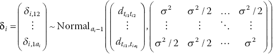
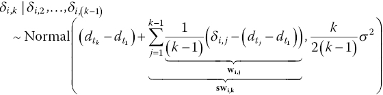
where δi is the vector of random effects, which follows a multivariate normal distribution, ai represents the number of arms in trial i (ai = 2, 3, …) and ![]() is as given in equation (2.9). Then the conditional univariate distribution (Raiffa and Schlaiffer, 2000) for the random effect of arm k > 2, given all arms from 2 to k − 1, is
is as given in equation (2.9). Then the conditional univariate distribution (Raiffa and Schlaiffer, 2000) for the random effect of arm k > 2, given all arms from 2 to k − 1, is

Either the multivariate distribution in equation (2.11) or the conditional distributions in equation (2.12) must be used to estimate the random effects for each multi-arm study so that the between-arm correlations between parameters are taken into account. We will use the formulation in equation (2.12) as it allows for a more generic code that works for trials with any number of arms. This general formulation is no different from the model presented by Higgins and Whitehead (1996) and provides another interpretation of the exchangeability assumptions. It is indeed another way of deducing the consistency relations: we may consider a connected network of M trials involving S treatments to originate from M S-arm trials, but with some of the arms missing at random, conditional on the trial design and choice of treatments, at randomisation (Section 1.5).
The WinBUGS code presented in Section 2.2.3.1 exactly instantiates the theory behind NMA that relates it to pairwise meta-analysis. Therefore it will analyse pairwise meta-analysis, indirect comparisons and NMA (including combined direct and indirect evidence) with or without multi-arm trials without distinction.
2.2.3 Worked Example: Network Meta-Analysis
We now synthesise the extended thrombolytics dataset presented in Table 2.1, comprising 36 RCTs comparing seven treatments. The treatment network is given in Figure 2.1. We define SK as our reference or ‘control’ treatment, coded 1, and number the other treatments according to Figure 2.1.
As before, we define rik as the number of events (deaths), out of the total number of patients in each arm, nik, for arm k of trial i, and assume that the data generation process follows the binomial likelihood described in equation (2.3). The probabilities of an event pik are modelled on the logit scale as
where μi are trial-specific baselines representing the log odds of the outcome in the ‘control’ treatment (i.e. the treatment in arm 1) and δik are the trial-specific LORs of an event on the treatment in arm k compared with the treatment in arm 1. Note that, in different trials, μi may represent the log odds of an event on different treatments. They are treated as nuisance parameters and given the (non-informative) prior distributions in equation (2.7). We set the relative effect of the treatment in arm 1 compared with itself to zero, ![]() , so that the treatment effects δik are only estimated when k > 1. For a random effects model, the trial-specific LORs come from the random effects distribution in equation (2.8).
, so that the treatment effects δik are only estimated when k > 1. For a random effects model, the trial-specific LORs come from the random effects distribution in equation (2.8).
For a fixed effects model, equation (2.13) is replaced by
where d11=0.
The basic parameters representing the pooled LOR of mortality for treatments 2, …, 7 compared with treatment 1 (the reference treatment) are assigned the prior distributions in equation (2.10). The prior distribution for the between-trial heterogeneity standard deviation σ is chosen as
which is appropriately wide in this case (see Section 2.3.2).
2.2.3.1 WinBUGS Implementation
The implementation of the NMA model with fixed treatment effects is given as follows:
WinBUGS code for NMA: Binomial likelihood, logit link, fixed effect model.
The # symbol is used for comments – text after this symbol is ignored by WinBUGS. Note that WinBUGS specifies the normal distribution in terms of its mean and precision.
The full code with data and initial values is presented in the online file Ch2_FE_Bi_logit.odc.
# Binomial likelihood, logit link# Fixed effect modelmodel{ # *** PROGRAM STARTSfor(i in 1:ns){ # LOOP THROUGH STUDIESmu[i] ~ dnorm(0,.0001) # vague priors for all trial baselinesfor (k in 1:na[i]) { # LOOP THROUGH ARMSr[i,k] ~ dbin(p[i,k],n[i,k]) # binomial likelihoodlogit(p[i,k]) <- mu[i] + d[t[i,k]] - d[t[i,1]] # model for linear predictor}}d[1]<-0 # treatment effect is zero for reference treatmentfor (k in 2:nt){ d[k] ~ dnorm(0,.0001) } # vague priors for treatment effects} # *** PROGRAM ENDS
Most of the lines in this fully generic (network) meta-analysis code are the same as in the previous code for pairwise meta-analysis with a fixed effect. The likelihood and prior distributions for mu[i] are the same, but now the loop covering all treatment arms needs to have k going from 1 to the total number of arms in that trial, which may be greater than 2, defined in na[i], loaded as data. The linear predictor now translates equation (2.14) into code where t[i,k] represents the treatment in arm k of trial i and d[k] = d1k. As before d[1] is set to zero, and prior distributions for all other d[k] are specified, with nt representing the total number of treatments compared in the network, which is given as data. Note that no special consideration is needed for multi-arm trials in fixed effects models since no random effects are estimated, and therefore no within-trial correlation needs to be accounted for.
The data structure is presented in the succeeding text and has two components: a list specifying the number of studies ns and treatments nt (in this example ns = 36, nt = 7) and the main body of data. Both sets of data need to be loaded for the model to run (see Section 2.2.1.2). The main body of data is in a vector format, and we need to allow for a three-arm trial. Three column places are therefore required to specify the treatments, t, the number of events, r, and the number of patients, n, in each arm; ‘NA’ indicates that values are missing for a particular cell: r[,1] and n[,1] are the numerators and denominators for the first arm, r[,2] and n[,2] are the numerators and denominators for the second arm and r[,3] and n[,3] represent the numerators and denominators for the third arm of each trial, respectively. We specify t[,1], t[,2] and t[,3] as the treatment number identifiers for the first, second and third arms of each trial, respectively, that is, they identify the treatments compared in each arm to which r and n correspond. We also add a column with the number of arms in each trial, na[]. Only the first trial in this dataset has three arms; all other trials have two arms. Trial identifiers are added as comments, which are ignored by WinBUGS:
# Data (Thrombolytics example)list(ns=36, nt=7)na[] t[,1] t[,2] t[,3] r[,1] n[,1] r[,2] n[,2] r[,3] n[,3] #ID year3 1 3 4 1472 20251 652 10396 723 10374 #GUSTO-1 19932 1 2 NA 3 65 3 64 NA NA #ECSG 19852 1 2 NA 12 159 7 157 NA NA #TIMI-1 19872 1 2 NA 7 85 4 86 NA NA #PAIMS 19892 1 2 NA 10 135 5 135 NA NA #White 19892 1 2 NA 887 10396 929 10372 NA NA #GISSI-2 19902 1 2 NA 5 63 2 59 NA NA #Cherng 19922 1 2 NA 1455 13780 1418 13746 NA NA #ISIS-3 19922 1 2 NA 9 130 6 123 NA NA #CI 19932 1 4 NA 4 107 6 109 NA NA #KAMIT 19912 1 5 NA 285 3004 270 3006 NA NA #INJECT 19952 1 7 NA 11 149 2 152 NA NA #Zijlstra 19932 1 7 NA 1 50 3 50 NA NA #Riberio 19932 1 7 NA 8 58 5 54 NA NA #Grinfeld 19962 1 7 NA 1 53 1 47 NA NA #Zijlstra 19972 1 7 NA 4 45 0 42 NA NA #Akhras 19972 1 7 NA 14 99 7 101 NA NA #Widimsky 20002 1 7 NA 9 41 3 46 NA NA #DeBoer 20022 1 7 NA 42 421 29 429 NA NA #Widimsky 20022 2 7 NA 2 44 3 46 NA NA #DeWood 19902 2 7 NA 13 200 5 195 NA NA #Grines 19932 2 7 NA 2 56 2 47 NA NA #Gibbons 19932 3 5 NA 13 155 7 169 NA NA #RAPID-2 19962 3 5 NA 356 4921 757 10138 NA NA #GUSTO-3 19972 3 6 NA 522 8488 523 8461 NA NA #ASSENT-2 19992 3 7 NA 3 55 1 55 NA NA #Ribichini 19962 3 7 NA 10 94 3 95 NA NA #Garcia 19972 3 7 NA 40 573 32 565 NA NA #GUSTO-2 19972 3 7 NA 5 75 5 75 NA NA #Vermeer 19992 3 7 NA 5 69 3 71 NA NA #Schomig 20002 3 7 NA 2 61 3 62 NA NA #LeMay 20012 3 7 NA 19 419 20 421 NA NA #Bonnefoy 20022 3 7 NA 59 782 52 790 NA NA #Andersen 20022 3 7 NA 5 81 2 81 NA NA #Kastrati 20022 3 7 NA 16 226 12 225 NA NA #Aversano 20022 3 7 NA 8 66 6 71 NA NA #Grines 2002END
In setting up the data structure, the maximum number of columns needed to define each variable is the maximum number of arms in the trials included in the dataset, that is, the maximum number specified in column na.
An important feature of the code presented is the assumption that the treatments are always presented in ascending (numerical) order and that treatment 1 is taken as the reference treatment. So, for example, the first row of data has the columns in order so that data for treatments 1, 3 and 4 are presented in the first, second and third columns, respectively, rather than having, for example, data for treatment 1, then 4 and then 3. Although this is not very important for the simple NMA models presented in this chapter and in Chapters 3 and 4 (the code will work regardless), it is crucial to have the data set up in this way to explore inconsistency (Chapter 7) and, when extending the model to include covariates (Chapter 8) or bias models (Chapter 9), to ensure the correct relative effects are estimated and appropriate assumptions are implemented.
We will run three chains using the following initial values:
# Initial values#chain 1list(d=c( NA, 0,0,0,0, 0,0), mu=c(0,0,0,0,0, 0,0,0,0,0, 0,0,0,0,0, 0,0,0,0,0, 0,0,0,0,0, 0,0,0,0,0, 0,0,0,0,0, 0))#chain 2list(d=c( NA, -1,-1,-1,-1, -1,-1), mu=c(-3,-3,-3,-3,-3, -3,-3,-3,-3,-3, -3,-3,-3,-3,-3, -3,-3,-3,-3,-3, -3,-3,-3,-3,-3, -3,-3,-3,-3,-3, -3,-3,-3,-3,-3, -3))#chain 3list(d=c( NA, 2,5,-3,1, -7,4), mu=c(-3,5,-1,-3,7, -3,-4,-3,-3,9,-3,-3,-4,3,5, -3, -2, 1, -3, -7, -3,5,-1,-3,7, -3,-4,-3,-3,0, -3, 5,-1,-3,7, -7))
Again note that d is a vector with seven components corresponding to the number of treatments being compared, but the initial value for the first component of vector d needs to be ‘NA’ since d[1] is set to zero and is therefore not estimated.
Running this model gives the following posterior summaries for the basic parameters, which represent the pooled LORs of mortality for all treatments compared with treatment 1 (SK). These are also summarised in Figure 2.4.
| node | mean | sd | MC error | 2.5% | median | 97.5% | start | sample |
| d[2] | −0.003229 | 0.03035 | 1.362E-4 | −0.06236 | −0.003249 | 0.0564 | 20001 | 150000 |
| d[3] | −0.1571 | 0.04349 | 2.77E-4 | −0.2427 | −0.1571 | −0.07212 | 20001 | 150000 |
| d[4] | −0.04324 | 0.04654 | 1.916E-4 | −0.135 | −0.04307 | 0.048 | 20001 | 150000 |
| d[5] | −0.1105 | 0.06014 | 3.667E-4 | −0.2288 | −0.1106 | 0.007321 | 20001 | 150000 |
| d[6] | −0.1518 | 0.0771 | 4.588E-4 | −0.3028 | −0.1517 | −6.668E-4 | 20001 | 150000 |
| d[7] | −0.4744 | 0.1006 | 4.5E-4 | −0.6722 | −0.474 | −0.2775 | 20001 | 150000 |
Figure 2.4 Extended thrombolytics example: caterpillar plot – from WinBUGS. Dots are posterior medians and lines represent 95% CrI for the log odds ratios of all treatments compared with SK, the reference treatment, from the fixed effects model. Numbers represent the treatment being compared (see Figure 2.1) and negative log odds ratios favour that treatment.
These LORs can be displayed in WinBUGS as a caterpillar plot, which can be obtained using the Inference→Compare… menu, by typing d in the ‘node’ box and clicking ‘caterpillar’. Treatment 7, PTCA, provides the largest reduction in mortality with posterior median of the LOR of −0.47 and 95% CrI (−0.67, −0.28).
Additional code can be added before the last closing brace to estimate all the pairwise LORs and ORs (i.e. for all treatments compared with every other), to generate ranking statistics and to calculate the probability that each treatment is the best treatment as well as the probabilities that each treatment is ranked 1st, 2nd, 3rd, and so on:
# pairwise ORs and LORs for all possible pairwise comparisonsfor (c in 1:(nt-1)) {for (k in (c+1):nt) {or[c,k] <- exp(d[k] - d[c])lor[c,k] <- (d[k]-d[c])}}# ranking on relative scalefor (k in 1:nt) {# rk[k] <- nt+1-rank(d[],k) # assumes events are “good”rk[k] <- rank(d[],k) # assumes events are “bad”best[k] <- equals(rk[k],1) # calculate probability that treat k is bestfor (h in 1:nt){ prob[h,k] <- equals(rk[k],h) } # calculate probability that treat k is h-th best}
In addition, given an assumption about the absolute effect of one treatment (see Chapter 5), it is possible to produce estimates of absolute effects on all treatments; to express the treatment effect on other scales such as the risk difference (RD), defined as the difference in probabilities of an event on treatment k compared with the reference treatment, and the relative risk (RR), defined as the ratio of the probabilities of an outcome on treatment k compared with treatment 1; or to calculate the number needed to treat (NNT), defined as 1/RD (Hutton, 2000; Deeks, 2002; Higgins and Green, 2008). An advantage of the Bayesian MCMC is that appropriate distributions, and therefore credible intervals, are automatically generated for all these quantities. This is achieved in WinBUGS by adding the following code:
# Provide estimates of treatment effects T[k] on the# natural (probability) scale, given a mean effect, meanA,# for ‘standard’ treatment 1, with precision precAA ~ dnorm(meanA,precA)for (k in 1:nt) { logit(T[k]) <- A + d[k] }
In this case, meanA and precA will be the assumed mean and precision of the log odds of mortality on treatment 1, respectively, and T[k] will represent the absolute probabilities of mortality on each treatment k = 1, …, 7. Given the information on the absolute probabilities of mortality T[1], other quantities can be calculated using the following code:
# Provide estimates of number needed to treat NNT[k]# Risk Difference RD[k] and Relative Risk RR[k],# for each treatment relative to treatment 1for (k in 2:nt) {# NNT[k] <- 1/(T[k] - T[1]) # assumes events are “good”NNT[k] <- 1/(T[1]- T[k]) # assumes events are “bad”RD[k] <- T[k] - T[1]RR[k] <- T[k]/T[1]}
We will assume the absolute probability of mortality on SK is 8% with 95% CrI from 7 to 10%, which is approximately equivalent to assuming that the log odds of mortality on SK follows a normal distribution with a mean of −2.39 and precision of 11.9. For considerations on how to estimate or elicit these values, see Chapter 5. These values can be given as data or replaced in the aforementioned code. We will include them in the data by changing the list to read
list(ns=36, nt=7, meanA=-2.39, precA=11.9)and loading that into WinBUGS.
The ORs of mortality for each treatment compared with every other can be obtained by monitoring node or. WinBUGS output for the fixed effects model is given in the succeeding text and summarised in Table 2.3 and Figure 2.5.
| node | mean | sd | MC error | 2.5% | median | 97.5% | start | sample |
| or[1,2] | 0.9972 | 0.03027 | 1.359E-4 | 0.9395 | 0.9968 | 1.058 | 20001 | 150000 |
| or[1,3] | 0.8554 | 0.0372 | 2.37E-4 | 0.7845 | 0.8547 | 0.9304 | 20001 | 150000 |
| or[1,4] | 0.9587 | 0.04463 | 1.838E-4 | 0.8737 | 0.9578 | 1.049 | 20001 | 150000 |
| or[1,5] | 0.897 | 0.05399 | 3.293E-4 | 0.7955 | 0.8953 | 1.007 | 20001 | 150000 |
| or[1,6] | 0.8617 | 0.06652 | 3.959E-4 | 0.7387 | 0.8592 | 0.9993 | 20001 | 150000 |
| or[1,7] | 0.6254 | 0.06305 | 2.823E-4 | 0.5106 | 0.6225 | 0.7577 | 20001 | 150000 |
| or[2,3] | 0.8586 | 0.04551 | 2.682E-4 | 0.7726 | 0.8573 | 0.9515 | 20001 | 150000 |
| or[2,4] | 0.9623 | 0.05353 | 2.266E-4 | 0.8613 | 0.9609 | 1.071 | 20001 | 150000 |
| or[2,5] | 0.9003 | 0.06062 | 3.591E-4 | 0.7876 | 0.8985 | 1.025 | 20001 | 150000 |
| or[2,6] | 0.8649 | 0.07175 | 4.158E-4 | 0.7323 | 0.8622 | 1.013 | 20001 | 150000 |
| or[2,7] | 0.6277 | 0.0657 | 2.987E-4 | 0.508 | 0.6245 | 0.7653 | 20001 | 150000 |
| or[3,4] | 1.122 | 0.06037 | 2.421E-4 | 1.008 | 1.121 | 1.245 | 20001 | 150000 |
| or[3,5] | 1.049 | 0.05817 | 2.914E-4 | 0.9411 | 1.048 | 1.169 | 20001 | 150000 |
| or[3,6] | 1.007 | 0.06435 | 2.826E-4 | 0.8875 | 1.005 | 1.139 | 20001 | 150000 |
| or[3,7] | 0.7316 | 0.07166 | 2.9E-4 | 0.6007 | 0.7284 | 0.8815 | 20001 | 150000 |
| or[4,5] | 0.9373 | 0.06649 | 3.24E-4 | 0.814 | 0.935 | 1.075 | 20001 | 150000 |
| or[4,6] | 0.9002 | 0.07511 | 3.575E-4 | 0.7619 | 0.8974 | 1.056 | 20001 | 150000 |
| or[4,7] | 0.6535 | 0.07034 | 2.867E-4 | 0.5259 | 0.6499 | 0.801 | 20001 | 150000 |
| or[5,6] | 0.9629 | 0.08145 | 3.988E-4 | 0.8129 | 0.9594 | 1.132 | 20001 | 150000 |
| or[5,7] | 0.6992 | 0.07725 | 3.395E-4 | 0.5598 | 0.6952 | 0.8615 | 20001 | 150000 |
| or[6,7] | 0.7293 | 0.08556 | 3.694E-4 | 0.5754 | 0.7245 | 0.911 | 20001 | 150000 |
Table 2.3 Extended thrombolytics example: median and 95% CrI for the odds ratios and between-study standard deviation (heterogeneity) from fixed and random effects models.
| X | Y | Fixed effect | Random effects | ||
| Median | 95% CrI | Median | 95% CrI | ||
| SK | t-PA | 1.00 | (0.94, 1.06) | 0.98 | (0.76, 1.10) |
| SK | Acc t-PA | 0.85 | (0.78, 0.93) | 0.85 | (0.69, 1.00) |
| SK | SK + t-PA | 0.96 | (0.87, 1.05) | 0.96 | (0.76, 1.23) |
| SK | r-PA | 0.90 | (0.80, 1.01) | 0.89 | (0.67, 1.06) |
| SK | TNK | 0.86 | (0.74, 1.00) | 0.85 | (0.60, 1.16) |
| SK | PTCA | 0.62 | (0.51, 0.76) | 0.61 | (0.47, 0.76) |
| t-PA | Acc t-PA | 0.86 | (0.77, 0.95) | 0.87 | (0.71, 1.16) |
| t-PA | SK + t-PA | 0.96 | (0.86, 1.07) | 0.98 | (0.79, 1.44) |
| t-PA | r-PA | 0.90 | (0.79, 1.03) | 0.91 | (0.71, 1.21) |
| t-PA | TNK | 0.86 | (0.73, 1.01) | 0.87 | (0.64, 1.33) |
| t-PA | PTCA | 0.62 | (0.51, 0.77) | 0.63 | (0.49, 0.84) |
| Acc t-PA | SK + t-PA | 1.12 | (1.01, 1.25) | 1.13 | (0.91, 1.50) |
| Acc t-PA | r-PA | 1.05 | (0.94, 1.17) | 1.04 | (0.83, 1.26) |
| Acc t-PA | TNK | 1.01 | (0.89, 1.14) | 1.00 | (0.77, 1.32) |
| Acc t-PA | PTCA | 0.73 | (0.60, 0.88) | 0.72 | (0.58, 0.88) |
| SK + t-PA | r-PA | 0.94 | (0.81, 1.08) | 0.92 | (0.65, 1.18) |
| SK + t-PA | TNK | 0.90 | (0.76, 1.06) | 0.89 | (0.60, 1.24) |
| SK + t-PA | PTCA | 0.65 | (0.53, 0.80) | 0.64 | (0.45, 0.83) |
| r-PA | TNK | 0.96 | (0.81, 1.13) | 0.96 | (0.70, 1.39) |
| r-PA | PTCA | 0.70 | (0.56, 0.86) | 0.70 | (0.53, 0.91) |
| TNK | PTCA | 0.72 | (0.58, 0.91) | 0.72 | (0.50, 0.99) |
| Heterogeneity (σ) | – | – | 0.064 | (0.003, 0.30) | |
Treatment definitions are given in Figure 2.1.

Figure 2.5 Extended thrombolytics example: summary forest plot – medians (dots) and 95% CrI (solid lines) for the ORs of all treatments compared with each other from the fixed effects model, plotted on a log scale. ORs < 1 favour the second treatment. Treatment definitions are given in Figure 2.1.
We can see that PTCA is better at reducing mortality than all other treatments, while, for example, Acc t-PA is slightly better than SK + t-PA, reducing the odds of mortality by about 12% with 95% CrI from 1 to 25%.
Note however that the estimates for the OR of mortality on PTCA compared with Acc t-PA are slightly different from those in Table 2.2 and the 95% CrI is narrower. This is expected since we are now using all the evidence in the network (both direct and indirect) to estimate this relative treatment effect.
A plot similar to Figure 2.5 can be obtained in WinBUGS by doing a ‘caterpillar’ plot of the parameter lor, although note that these will be the LORs. See Exercise 2.1.
The probabilities that each treatment is ranked 1st, 2nd, …, 7th are shown in Figure 2.6. Peaks in these figures indicate the most likely rank for that treatment, and the probabilities of each rank can be read on the vertical axis.

Figure 2.6 Extended thrombolytics example: probability that each treatment is ranked 1–7 for fixed and random effects models. Treatment definitions are given in Figure 2.1.
As expected, PTCA has a very high probability of being the best treatment, and so the probability that it is ranked 1st is close to 100%. Among the other treatments, Acc t-PA has probability of 42% being ranked 2nd and 48% of being ranked 3rd, and TNK also has about 43% probability of being ranked 2nd, suggesting these may be the best alternatives to PTCA, when it is not available. This agrees with the ORs in Figure 2.5, where apart from PTCA, Acc t-PA and TNK are the only other treatments that are favoured over the alternatives, and there seems to be no advantage of one over the other. The absolute probabilities, ranks and probabilities of being the best for all treatments are shown in Table 2.4.
Table 2.4 Extended thrombolytics example: results from the fixed effects network meta-analysis model.
| Treatment | Probability of 35 day mortality | Rank | Pr(best) | |||
| Median | 95% CrI | Mean | Median | 95% CrI | ||
| SK | 0.08 | (0.05, 0.14) | 6.31 | 6 | (5, 7) | 0.00 |
| t-PA | 0.08 | (0.05, 0.14) | 6.13 | 6 | (4, 7) | 0.00 |
| Acc t-PA | 0.07 | (0.04, 0.12) | 2.69 | 3 | (2, 4) | 0.00 |
| SK + t-PA | 0.08 | (0.05, 0.13) | 5.13 | 5 | (3, 7) | 0.00 |
| r-PA | 0.08 | (0.04, 0.13) | 3.75 | 4 | (2, 6) | 0.00 |
| TNK | 0.07 | (0.04, 0.12) | 3.00 | 3 | (2, 6) | 0.00 |
| PTCA | 0.05 | (0.03, 0.09) | 1.00 | 1 | (1, 1) | 1.00 |
Treatment definitions are given in Figure 2.1.
The implementation of the random effects model accounting for the correlations in multi-arm trials is as follows:
WinBUGS code for NMA: Binomial likelihood, logit link, random effects model.
The # symbol is used for comments – text after this symbol is ignored by WinBUGS. Note that WinBUGS specifies the normal distribution in terms of its mean and precision.
The full code with data and initial values is presented in the online file Ch2_RE_Bi_logit.odc.
# Binomial likelihood, logit link# Random effects model for multi-arm trialsmodel{ # *** PROGRAM STARTSfor(i in 1:ns){ # LOOP THROUGH STUDIESw[i,1] <- 0 # adjustment for multi-arm trials is zero for control armdelta[i,1] <- 0 # treatment effect is zero for control armmu[i] ~ dnorm(0,.0001) # vague priors for all trial baselinesfor (k in 1:na[i]) { # LOOP THROUGH ARMSr[i,k] ~ dbin(p[i,k],n[i,k]) # binomial likelihoodlogit(p[i,k]) <- mu[i] + delta[i,k] # model for linear predictor}for (k in 2:na[i]) { # LOOP THROUGH ARMSdelta[i,k] ~ dnorm(md[i,k],taud[i,k]) # trial-specific LOR distributionsmd[i,k] <- d[t[i,k]] - d[t[i,1]] + sw[i,k] # mean of LOR distributions (multi-arm trial correction)taud[i,k] <- tau *2*(k-1)/k # precision of LOR distributions (with multi-arm trial correction)w[i,k] <- (delta[i,k] - d[t[i,k]] + d[t[i,1]]) # adjustment for multi-arm RCTssw[i,k] <- sum(w[i,1:k-1])/(k-1) # cumulative adjustment for multi-arm trials}}d[1] <- 0 # treatment effect is zero for reference treatmentfor (k in 2:nt){ d[k] ~ dnorm(0,.0001) } # vague priors for treatment effectssd ~ dunif(0,2) # vague prior for between-trial SD.tau <- pow(sd,-2) # between-trial precision = (1/between-trial variance)} # *** PROGRAM ENDS
Readers should compare this code with the random effects code for pairwise meta-analysis and the fixed effects code for NMA and note the similarities. The main difference in this code is the implementation of the conditional univariate normal distributions for the trial-specific random effects given in equation (2.12).
We have coded the mean of the random effects normal distribution as md (WinBUGS does not allow algebraic expressions in distributions) and defined md as ![]() where swik is the adjustment for the conditional normal distribution given as follows:
where swik is the adjustment for the conditional normal distribution given as follows:
and taud is the adjusted precision for the conditional univariate normal, that is, the inverse of the aforementioned variance. We set w[i,1] to zero so that the code reduces to a simple univariate normal distribution (equation (2.8)) for two-arm trials.
Changes to the initial values are also required. Initial values need to be specified for the between-study heterogeneity sd, and WinBUGS can be left to generate initial values for the parameter delta, as before.
Results from the random effects model are given in Table 2.3. The posterior median of the between-study standard deviation is small compared with the size of the treatment effect of PTCA (Table 2.3), and its posterior distribution is concentrated around small values (Figure 2.7). We might therefore question whether a random effects model is really necessary here. Model comparison and model choice will be discussed in Chapter 3.

Figure 2.7 Extended thrombolytics example: posterior distribution of the between-study standard deviation – from WinBUGS.
The posterior distribution of the between-study standard deviation (Figure 2.7) is far from the uniform distribution between zero and two that was set up as prior. This confirms that updating has taken place and that the prior distribution was not too restrictive (see Section 2.3.2 for more details). We should also note that the distribution is slightly different from that in Figure 2.3, since we are now using more evidence to estimate this parameter. In this case this has meant that the distribution is slightly narrower and concentrated around smaller values (see Section 2.3.2).
2.3 Technical Issues in Network Meta-Analysis
The use of the WinBUGS Bayesian MCMC software has advantages but it also requires some care. Users are strongly advised to acquire a good understanding of the Bayesian theory (Spiegelhalter et al., 2004) and to follow advice given in the WinBUGS manual and book (Lunn et al., 2013). Particular care must be taken in checking convergence, and we suggest that at least three chains are run, starting from widely different (yet sensible) initial values. The diagnostics recommended in the literature should be used to check convergence (Gelman, 1996; Brooks and Gelman, 1998). Users should also ensure that, after convergence, each chain is sampling from the same posterior distribution. Posteriors should be examined visually for spikes and unwanted peculiarities, and both the initial ‘burn-in’ and the posterior samples should be conservatively large (Lunn et al., 2013). The number of iterations used for both must be always reported.
Beyond these warnings, which apply to all Bayesian MCMC analyses, NMA models have particular properties that require careful examination.
2.3.1 Choice of Reference Treatment
While the likelihood is not altered by a change in which treatment is taken to be ‘treatment 1’, the choice of the reference treatment can sometimes affect the posterior estimates because prior distributions cannot be totally non-informative. However, for the vague prior distributions we suggest throughout for μi and d1k (see Section 2.3.2), we expect the effect to be negligible. Choice should therefore be based on ease of interpretation, with placebo or a standard treatment usually taken as treatment 1. In larger networks, it is preferable to choose as treatment 1 a treatment that is in the ‘centre’ of the network. In other words, choose the treatment that has been trialled against the highest number of other treatments. The purpose of this is to reduce strong correlations that may otherwise be induced between mean treatment effects for pairs of treatments, which can slow convergence and make for inefficient sampling from the posterior distribution, although in theory if enough samples are collected, results can still be used for inference.
2.3.2 Choice of Prior Distributions
We recommend vague or flat prior distributions, such as Normal(0,1002), throughout for μi and d1k. Informative prior distributions for relative effect measures would require special justification but can be easily implemented by specifying, for example, d[k]~dnorm(0,0.1) to represent a normal distribution with mean 0 and precision 0.1 (variance = 10) for the relative effects of all treatments compared with the reference. Normal prior distributions are appropriate when the treatment effects are defined on a continuous scale ranging from minus to plus infinity (such as the LORs). For treatment effects defined on scales with a different range, different prior distributions need to be considered – see Section 2.3.3.
It has become standard practice to also set vague prior distributions for the between-trial variances. For binomial with logit link models, the usual practice is to place a uniform prior distribution on the standard deviation, for example, σ ~ Uniform(0,2). The upper limit of 2 represents a huge range of trial-specific treatment effects (Spiegelhalter et al., 2004, table 5.2). For example, if the median treatment effect was an OR of 1.5 (i.e. LOR of 0.405), then we would expect 95% of trials to have true ORs between 0.2 and 11 (calculated as exp(0.405 ± 2)). The posterior distribution of σ should always be inspected to ensure that it is sufficiently different from the prior distribution as this would otherwise indicate that the prior distribution is dominating the data and no posterior updating has taken place. This can be done in WinBUGS by plotting the posterior density of sd (see Figures 2.1 and 2.7) or by exporting the simulated values into other software and plotting them there.
An alternative approach, which was once popular but has since fallen out of favour, is to set a vague gamma prior distribution on the precision, for example, 1/σ 2 ~ Gamma(0.001,0.001). This approach gives a low prior weight to unfeasibly large σ on the logit scale but is actually quite informative when low values of σ are possible, and inferences are sensitive to the specific parameters of the gamma distribution chosen when data are sparse (Gelman, 2006). One specific disadvantage is that this puts considerable weight on values of σ near zero but, on the other hand, it rules out values of σ at zero. This may be desirable, because it is not uncommon, particularly when data are sparse, that MCMC sampling can ‘get stuck’ at σ ≈ 0, leading to spikes in the posterior distribution of both σ and the treatment effect parameters d1k. In these cases a gamma prior distribution may improve numerical stability and speed convergence. Half-normal prior distributions constrained to be positive can also be useful when data are sparse.
However they are formulated, there are major disadvantages in routinely using vague prior distributions for the between-study heterogeneity, although this has become a widely accepted practice. In the absence of large numbers of large trials for at least one comparison (at least four or five trials have been suggested as a minimum (Gelman, 2006)), the posterior distribution of σ will be poorly identified and likely to include values that, on reflection, are implausibly high or, possibly, implausibly low. Two further alternatives may be useful when there is insufficient data to adequately estimate the between-trial variation. The first is the use of external data (Higgins and Whitehead, 1996). If there is insufficient data in the meta-analysis, it may be reasonable to use an estimate for σ from a larger meta-analysis on the same trial outcome involving a similar treatment for a similar condition. The posterior distribution, or a posterior predictive distribution (Lunn et al., 2013) (see also Chapters 3 and 8), from such an analysis could be used to approximate an informative prior distribution. Alternatively, prior distributions derived from large numbers of meta-analyses can be used, with the appropriate prior distribution chosen depending on the outcome type and the type of treatments being compared (Turner et al., 2012, 2015b). Chapter 6 discusses issues caused by sparse data in more detail.
If there are no data on similar treatments and outcomes that can be used, an informative prior distribution can be elicited from a clinician who knows the field. This can be done by posing the question in this way: ‘Suppose we accept that different trials, even if infinitely large, can produce different effect sizes. If the average effect was an OR of 1.8 [choose a plausible average], what do you think an extremely high and an extremely low effect would be, in a very large trial?’ Based on the answer to this, it should be possible, by trial and error, to construct an informative gamma prior distribution for 1/σ2 or a normal prior distribution for σ, subject to σ > 0 (half-normal). For further discussion of prior distributions for variance parameters, see Lambert et al. (2005) and Spiegelhalter et al. (2004).
There can be little doubt that the vague prior distributions that are generally recommended for the heterogeneity parameter produce posterior distributions that are biased upwards. The extent of the bias is likely to be greater when the true variance is low and when there are few data: either few trials or small trials. However, this is also a problem when using frequentist estimators. Although we can be reassured that the bias tends to be conservative, ultimately it may be preferable to use informative prior distributions, perhaps tailored to particular outcomes and disease areas, based on studies of many hundreds of meta-analyses (Turner et al., 2012; Rhodes et al., 2015; Turner et al., 2015b). An easier approach might be to identify a large meta-analysis of other treatments for the same condition and using the same outcome measures and use the posterior distribution for the between-trial heterogeneity from this meta-analysis to inform the current analysis (Dakin et al., 2010).
Whichever prior distribution is chosen, it can be easily implemented in WinBUGS by changing the relevant lines of code. See Exercise 2.4.
2.3.3 Choice of Scale
The logit model presented in this chapter assumes linearity of effects on the log odds scale. It should be emphasised that it is important to use a scale in which effects are additive, as is required by the linear model (Deeks, 2002; Caldwell et al., 2012). Choice of scale can be guided by goodness of fit (see Chapter 3) or by lower between-study heterogeneity, but there is seldom enough data to make this choice reliably, and logical considerations may play a larger role (Caldwell et al., 2012). Quite distinct from choice of scale for modelling is the issue of how to report treatment effects. Thus, while one might assume linearity of effects on the log odds scale, the investigator, given information on the absolute effect of one treatment, is free to derive treatment effects with 95% CrI on other scales, such as RD, RR or NNT using the additional code provided in Section 2.2.3.1. Therefore, the most appropriate scale for each problem should be chosen based on statistical and logical considerations and not on reporting preferences.
Warn et al. (2002) suggest models for pairwise meta-analysis of binomial data using the RD and log RR while still using the arm-based binomial likelihood in equation (2.3). The difficulty in modelling the probabilities on these scales is that while the LOR is unbounded, that is, it can take any value between plus and minus infinities, the RD must be between −1 and 1 and the log RR is bounded by the probability of an event, the risk, in the reference group, for each study. Thus the model must be constrained to ensure the probabilities of an event in each arm of each study remain between zero and one. To model binomial data on the RD scale, equation (2.13) is replaced by (Warn et al., 2002)
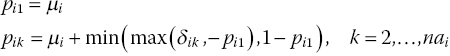
which ensures that ![]() . The random effects distribution is the same as in equation (2.8), but the basic parameters are now the RD relative to treatment 1 which are bounded between −1 and 1. For a fixed effects model, we write
. The random effects distribution is the same as in equation (2.8), but the basic parameters are now the RD relative to treatment 1 which are bounded between −1 and 1. For a fixed effects model, we write
The prior distributions in equation (2.10) are replaced with ![]() . The μi now represent the probability of an event in arm 1 of trial i, which must also lie between zero and one, so they are given Uniform(0,1) prior distributions. The prior distribution for the between-study heterogeneity can be the same as presented in equation (2.15) or a suitable alternative (see Section 2.3.2).
. The μi now represent the probability of an event in arm 1 of trial i, which must also lie between zero and one, so they are given Uniform(0,1) prior distributions. The prior distribution for the between-study heterogeneity can be the same as presented in equation (2.15) or a suitable alternative (see Section 2.3.2).
To model binomial data on the log RR scale, equation (2.13) is replaced by (Warn et al., 2002)
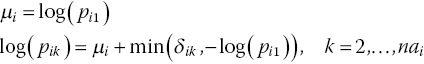
with ![]() , which ensures that
, which ensures that ![]() . The random effects distribution is the same as in equation (2.8), but the basic parameters are now the log RR relative to treatment 1. For a fixed effects model, we use equation (2.16). Warn et al. (2002) suggest that normal prior distributions with mean zero and variance of 10 are sufficiently vague for d1k. The μi now represent the log risks in the control arm, that is, the log of the probability of an event in arm 1 of trial i. Prior distributions can be given by noting that
. The random effects distribution is the same as in equation (2.8), but the basic parameters are now the log RR relative to treatment 1. For a fixed effects model, we use equation (2.16). Warn et al. (2002) suggest that normal prior distributions with mean zero and variance of 10 are sufficiently vague for d1k. The μi now represent the log risks in the control arm, that is, the log of the probability of an event in arm 1 of trial i. Prior distributions can be given by noting that ![]() is the probability of an event in arm 1 of trial i, which must lie between zero and one. Thus Uniform(0,1) prior distributions can be given to pi1. The prior distribution for the between-study heterogeneity can be the same as presented in equation (2.15). For further details on the WinBUGS implementation of these models, see Warn et al. (2002) and Exercise 2.5.
is the probability of an event in arm 1 of trial i, which must lie between zero and one. Thus Uniform(0,1) prior distributions can be given to pi1. The prior distribution for the between-study heterogeneity can be the same as presented in equation (2.15). For further details on the WinBUGS implementation of these models, see Warn et al. (2002) and Exercise 2.5.
Although attractive, these models can pose some computational and interpretation challenges when there are studies with zero events or with 100% events. In particular the RD model can cause numerical problems when the relative treatment effects are close to −1 or 1, which can happen by chance, particularly during the burn-in period. Some workarounds are possible, including using a slightly more restrictive prior distribution for the basic parameters, for example, uniform between −0.9999 and 0.9999, to avoid very extreme values being sampled (see Exercise). Warn et al. (2002) provide a thorough discussion of the issues and suggested workarounds.
2.3.4 Connected Networks
The models described assume that the network of treatments is connected, that is, there is a path leading from each treatment to every other. If this is not the case, steps should be taken to connect the network before inference on all relative effects can be made (see Section 1.6). However, the models presented here will still run for disconnected networks, and relative effects will be produced by WinBUGS. For disconnected treatments the relative effects produced will reflect only the prior distribution given (typically vague) as that is the only available information. Careful inspection of the output will immediately show this, as some parameters will have very large posterior variances, reflecting the variance in the prior distributions.
Network connectivity should always be checked before putting the data through the WinBUGS code. Particular care should be taken when there are studies with zero cells to ensure there is information on all contrasts – see Chapter 6 for further details. However, if this step is missed or performed incorrectly, inspecting the posterior distributions obtained for the basic parameters (d) will show these to be very wide and not updated from the prior distributions, highlighting the problem.
2.4 Advantages of a Bayesian Approach
Readers should note that implementation of NMA models with fixed or random effects, consistency equations and incorporating multi-arm correlations are straightforward in WinBUGS. Furthermore, the code presented in this chapter can be easily adapted to other data types (Chapter 4) and implemented to other models, such as those including a covariate or bias adjustment terms (Chapters 8 and 9).
An advantage of the Bayesian model with binomial likelihood is that exact arm-based likelihoods are used, and this means special precautions do not usually need to be taken in the case of the occasional trial with a zero cell count, since a binomial likelihood with a zero cell is allowed by WinBUGS (see Chapter 6). Chapters 4 and 10 extend this approach to other data types where, again, the arm-based likelihoods are used whenever possible. This is a major strength of the Bayesian MCMC approach, because some popular frequentist approaches for LORs have to add an arbitrary constant, usually 0.5, to cells in order to obtain non-infinite estimates of treatment effects and non-infinite variance, but in so doing they generate biased estimates of effect size (Sweeting et al., 2004; Bradburn et al., 2007). Simulation studies on fixed effect estimators (Sweeting et al., 2004) have also shown that Bayesian MCMC has performed well, ranks with Mantel–Haenszel (Mantel and Haenszel, 1959) and Exact method (Fleiss, 1994) estimators and is superior to the Peto method (Yusuf et al., 1985) and inverse-variance weighting in a wide range of situations.
However, in extreme cases where several trials have zero cells and many of the trials are small, the models we have recommended can be numerically unstable, either failing to converge or converging to a posterior distribution with very high standard deviation for some of the treatment effects. This is unlikely to happen with fixed effects models, and it can often be remedied in random effects models by using a (more) informative prior distribution on the variance parameter. The last resort, recognising the assumptions being made, is to put a random effects model on the trial-specific baselines μi as well as the relative treatment effects d1k. See Chapter 5 for comments on this model and Chapter 6 for a thorough discussion of issues with sparse data and zero cells.
A specific problem arises in sparse networks, in which, for example, there is only one trial making the comparison X versus Y, and treatment Y only appears in this one trial. If the trial contains a zero cell, it may not be possible to estimate a treatment effect, and the output for that relative effect will resemble that of a disconnected network, that is, the prior distribution will not have been updated (Section 2.3.4). Trials with zero cells in both arms do not contribute evidence on the treatment effect and can be excluded, unless a model has been assumed for the trial-specific baselines. See Chapter 6 for further details.
Furthermore, in random effects models, the MCMC implementation proposed in this book automatically takes into account the uncertainty in the between-study heterogeneity parameter σ2. While this is also possible using frequentist approaches (Zelen, 1971; Hardy and Thompson, 1996; Biggerstaff and Tweedie, 1997), it is rarely done in practice, and instead σ2 is estimated and then assumed to be fixed and known for the purpose of computing the pooled treatment effects. By taking into account the uncertainty in σ2 and propagating that to the uncertainty in the posterior distributions of the relative effects, the Bayesian implementation proposed here better reflects the overall uncertainty in the estimates, which is a crucial factor in decision-making (see Chapter 5).
2.5 Summary of Key Points and Further Reading
We have shown how to implement the two-treatment meta-analysis models with binary data in WinBUGS and that it is relatively simple to extend these models to meta-analysis of any number of trials on the same S ≥ 2 comparators. In this framework, extension of the exchangeability assumption required for pairwise meta-analysis automatically delivers the assumption required for meta-analysis with more than two treatments, and vice versa.
In this chapter we have shown how to obtain the outputs generally required for reporting the results of an NMA. Different ways of summarising and presenting the results in tables and figures have been proposed (Chaimani et al., 2013a; Tan et al., 2014). For example, similar to the rank plots in Figure 2.6, the surface under the curve has been suggested as a summary (Salanti et al., 2011), and this can be calculated in WinBUGS. An analysis of the network geometry or of the relative weight contributions of each contrast to the pooled result have also been suggested as useful outputs, and readers are referred to the original references for more details (Salanti et al., 2008b; König et al., 2013).
The models with fixed and random effects have been implemented in WinBUGS using code that will work for any number of treatments and trials with any number of arms, when the outcome is binary. The code respects the randomisation in the original studies by modelling relative treatment effects and accounts for the correlation in trials with more than two arms in random effects models.
The issues of model fit and model choice are crucial to valid inference and decision-making and are explored in Chapter 3. Chapter 4 extends the model presented for binomial data with a logit link to the framework of generalised linear models, where the basic modelling framework stays the same, but the likelihood and link functions change to allow synthesis of different data types. Chapters 8 and 9 cover issues of heterogeneity, looking at meta-regression and treatment effects in subgroups and methods for bias adjustment, including publication bias and the so-called ‘small-study bias’. In addition, Chapter 8 considers models where restrictions are placed on the relative treatment effects, for example, that they are exchangeable within class or additive. The synthesis of both direct and indirect evidence on the same contrast also raises questions about inconsistency between evidence sources (Chapter 1), which will be addressed in Chapter 7. Further considerations on the validity of the proposed approach to synthesis are made in Chapter 12.
Bayesian analysis is by no means a panacea: one area that clearly deserves more work is how to specify a ‘vague’ prior distribution for the variance parameter. Readers are referred to Section 2.3.2 and also to standard Bayesian textbooks (Bernardo and Smith, 1994; Gelman et al., 2004; Spiegelhalter et al., 2004) for general discussions of this issue.
2.6 Exercises
- 2.1 Using the extended thrombolytics example, run the WinBUGS code provided to obtain the values presented in Table 2.3.
- Draw a plot similar to Figure 2.5 in WinBUGS by plotting
lor. What are the main differences between the two plots? - Monitor the variable
rkand plot its density for both the fixed and random effects models and compare with Figure 2.6.
- Draw a plot similar to Figure 2.5 in WinBUGS by plotting
- 2.2 Using the extended thrombolytics example, compare the OR for PTCA relative to Acc t-PA for the fixed effect pairwise meta-analysis (Table 2.2) with the corresponding OR in Table 2.3. Can you explain any differences in effect size and uncertainty?
- 2.3 Using the extended thrombolytics example, suppose there was a new study comparing treatment 3 (Acc t-PA) with a new (fictitious) treatment 8, where there were 5 deaths out of 32 patients randomised to treatment 3 and 8 deaths out of 35 patients randomised to treatment 8.
- How would the network plot in Figure 2.1 change with the inclusion of the new study?
- How do you expect this study to influence the estimates of the relative effects for the other treatments? If a random effects model was fitted, how would you expect the between-study heterogeneity to change? Confirm your answers by running the random effects model with the new study included.
- Now suppose there was a further study added comparing the new (fictitious) treatment 8 with treatment 7 (PTCA). Would this be expected to influence the other relative effects and the between-study heterogeneity (in a random effects model)?
- 2.4 *Table IV of Turner et al. (2015b) lists a series of lognormal prior distributions for the between-study variance, based on empirical data, for different outcome and comparison types. Using the extended thrombolytics example, fit the random effects network meta-analysis model using an informative prior distribution for the between-study heterogeneity, as suggested by Turner et al. (2015b).
- Decide on the most appropriate distribution to consider given the outcome and comparison types presented in this example. (Hint: if there is more than one comparison type, use multiple prior distributions and compare the results.)
- Use the WinBUGS Help for details on how to code a lognormal distribution and change the code provided to implement the new prior distribution(s). Note that the prior distributions suggested by Turner et al. (2015b) are for the between-study variance.
- Inspect the posterior distribution of
sdand compare with Figure 2.3. Note any changes in relative treatment effects compared with those in Table 2.3.
- 2.5 *Using the extended thrombolytics example, adapt the standard network meta-analysis code to fit fixed and random effects models using the risk difference and the log relative risk as the scale of the linear predictor as suggested by Warn et al. (2002) (Section 2.3.3). Take care to ensure appropriate prior distributions are given and that the initial values are within the bounds of the prior distributions. Note that for the random effects model on the risk difference, you may need to reduce the range of the uniform prior distributions for the basic parameters.
- Compare the risk difference/relative risk estimates with those obtained by using the logit link and then transforming the ORs (Section 2.2.3.1). Compare also the probability that PTCA is the best treatment and the between-study heterogeneity in the random effects models.