
Appendices
Appendix A Sample R Code to Obtain Adjusted Standard Errors Using Netmeta (Chapter 7)
Available as electronic file in AppAnetmetascript.R.
# Full Thrombo example: load datadatanet <- read.csv("DataThromb.csv", header=TRUE, sep=",")TreatCodes <- read.csv("TreatCodes.csv", header=TRUE, sep=",")print(TreatCodes)######################################################## Obtain reduced weights for FE model######################################################library(netmeta)# Gerta Rücker, Guido Schwarzer, Ulrike Krahn and Jochem König (2016).# netmeta: Network Meta-Analysis using Frequentist Methods. R package# version 0.9-1. https://CRAN.R-project.org/package=netmetap1 <- pairwise(treat=list(t1, t2, t3),event=list(r1, r2, r3),n=list(n1,n2,n3),data=datanet, studlab=study)print(p1)# net1 <- netmeta(TE, seTE, treat1,treat2,studlab, data=p1)print(net1)# study 1s1 <- net1$studlab == 1 # choose study 1net1$seTE[s1] # Unadjusted standard errorsnet1$seTE.adj[s1] # Adjusted standard errors# study 6s2 <- net1$studlab == 6 # choose study 6net1$seTE[s2] # Unadjusted standard errors (as given in the data)net1$seTE.adj[s2] # Adjusted standard errors## DATA FOR WinBUGS: treatment difference and adjusted st. errors# change sign to be log-OR of treat 2 compared to 1cbind(t1=c(net1$treat1[s1], net1$treat1[s2]),t2=c(net1$treat2[s1], net1$treat2[s2]),y2=c(-net1$TE[s1], -net1$TE[s2]),se2=c(net1$seTE.adj[s1], net1$seTE.adj[s2]),study=c(rep(1,3), rep(6,3)))## END
Appendix B Derivation of Prior Distribution for Heterogeneity Parameter Used in Certolizumab Example: Random Effects Model with Covariate (Chapter 8)
We want to find a half-normal distribution, that is, a Normal(0,m 2) distribution, truncated to take only positive values, which expresses the prior belief that 95% of trials will give odds ratios within a factor of 2 from the estimated median odds ratio. Assuming no treatment effect (without loss of generality), we have
and we want to find m that defines a prior distribution for σ such that the 95% CrI for OR = exp(δ) is approximately (0.5, 2).
Implementing this in WinBUGS gives the following code:
model{delta ~ dnorm(0,tau)tau <- pow(sd,-2)prec <- pow(m,-2)sd ~ dnorm(0,prec)I(0,)OR <- exp(delta)}
Thus, we want to find m such that the 95% CrI for OR is approximately (0.5, 2). We can do this simply by experimentation with different values of m, given as data. When we set m to 0.32: list(m=0.32), we get the following results:
| node | mean | sd | MC error | 2.5% | median | 97.5% | start | sample |
| OR | 1.051 | 0.4147 | 0.001756 | 0.4924 | 0.9998 | 1.985 | 5001 | 50000 |
| delta | –0.002994 | 0.3186 | 0.001378 | –0.7084 | –1.602E–4 | 0.6857 | 5001 | 50000 |
| sd | 0.2554 | 0.193 | 8.714E–4 | 0.01026 | 0.2155 | 0.718 | 5001 | 50000 |
which are close enough to the desired values. Thus we chose σ ~ Half-![]() as the prior in the example given in Section 8.4.2 (equation 8.7).
as the prior in the example given in Section 8.4.2 (equation 8.7).
Appendix C Reconstructing Data from Published Kaplan–Meier Curves (Chapter 10)
C.1 Details for the Guyot IPD Reconstruction Algorithm
Data inputs required are the coordinates extracted from the Kaplan–Meier (KM) curve: times U
j
where ![]() and corresponding survival probabilities S
j
for
and corresponding survival probabilities S
j
for ![]() points on the KM curve. These points should include the times at which numbers at risk are reported below the curve, must capture all steps in the curve, and adjustments to the extracted coordinates to ensure the survival probabilities are decreasing with time. The curve is split into
points on the KM curve. These points should include the times at which numbers at risk are reported below the curve, must capture all steps in the curve, and adjustments to the extracted coordinates to ensure the survival probabilities are decreasing with time. The curve is split into ![]() intervals, defined by the points where number at risk are reported below the curves, where
intervals, defined by the points where number at risk are reported below the curves, where ![]() and
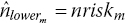
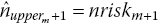
and ![]() give the extracted coordinates corresponding to the lower and upper ends of interval m, respectively. The reported number at risk at the start of interval m is nrisk
m
. If reported, the total number of events, totevents, is also used by the algorithm.
give the extracted coordinates corresponding to the lower and upper ends of interval m, respectively. The reported number at risk at the start of interval m is nrisk
m
. If reported, the total number of events, totevents, is also used by the algorithm.
Here we assume that the number at risk is reported at the start of the study and at least one other time point and that the total number of events is also reported. See Guyot et al. (2012) for adaptations to the algorithm when this is not the case. We assume the number of censored individuals on each interval is not available. We therefore estimate the number of censored individuals on each interval by an iterative process to match the predictions from the inverted KM equations with the reported number at risk at the ends of each interval. We assume that censoring occurs at a constant rate within each of the time intervals, which seems reasonable if the censoring pattern is non-informative (each subject has a censoring time that is statistically independent of their failure time).
The algorithm is made up of the following steps:
-
Step 1. Form an initial guess for the number censored on interval m. If there were no censored individuals on interval m, then the number at risk at the beginning of interval
 would berounded to the nearest integer, where
 is the probability of being alive at start of interval
  given alive at the start of interval m.
 An initial guess for the number censored on interval m is the difference between the reported number at risk at the beginning of interval
 and the number at risk under no censoring:

-
Step 2. Distribute the
 censor times,
  , evenly over interval m:The number of censored observations between extracted KM coordinates j and
 , cên
j
, is found by counting the number of estimated censor times,
, cên
j
, is found by counting the number of estimated censor times,  , that lie between time U
j
and
, that lie between time U
j
and  .
. -
Step 3. The estimated number of events, ê
j
, at each extracted KM coordinate, j, and hence estimated number at risk at the next coordinate,
 , can then be calculated. The KM equations givewhere last(j) is the last coordinate where we estimate that an event occurred prior to coordinate j. This is necessary because the KM equations assume that intervals are defined by the event times.
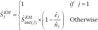
Rearranging gives
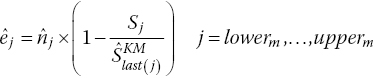
rounded to the nearest integer.
The number of patients at risk at each extracted coordinate, j, is then obtained:

where at the start of the interval we set
 . This produces an estimated number at risk at the start of the following interval
  .
. -
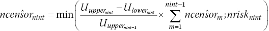
Step 4. If
 then readjust the estimated number of censored observations in interval m toRepeat steps 2–3 iteratively until estimated and published number at risk match (i.e.
 ).
). -
Step 5. If
 is not the last interval, repeat steps 1–4 for the following interval.
 -
Step 6. In published RCTs, there is generally no number at risk published at the end of the last interval, nint. We assume that the censored rate on the last interval equals the average censor rate from the previous intervals, so the estimated censored individuals on the last interval is the average censor rate multiplied by the length of the last interval, constrained to be less than or equal to the number of patients at risk at the start of the last interval. This assumption is written assteps 2–3 are then run for the last interval.
-
Step 7. If the estimated total number of events prior to the beginning of the last interval
 is greater or equal to the reported total number of events, totevents, we assume that no more events or censoring occurs
-
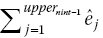
Step 8. If
 is less than totevents, readjust the estimated number of censored observations,
  , by the difference in total number of eventsThen rerun steps 2–3, 8 for the last interval, nint, until the estimated total number of events,
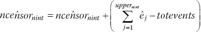
 , or until
 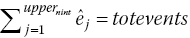 , but the total number of censoring in the last interval,
  , becomes equal to zero.
C.2 Details of the Algorithm for Constructing Interval Data
The algorithm described here is based on the method used by Jansen and Cope (2012) to create interval data. The available follow-up time period for each arm of each trial is divided in w sequential short time intervals ![]() with u
1 = 0. For each time interval
with u
1 = 0. For each time interval ![]() , the conditional survival probability is calculated based on the scanned survival proportions according to
, the conditional survival probability is calculated based on the scanned survival proportions according to ![]() . If there is no survival proportion available for a specific time point, a corresponding estimate for S(u
m
) can be obtained by linear interpolation of the first available extracted scanned survival proportions before and after this time point.
. If there is no survival proportion available for a specific time point, a corresponding estimate for S(u
m
) can be obtained by linear interpolation of the first available extracted scanned survival proportions before and after this time point.
Given the reported numbers at risk n m at the beginning of the mth interval and the event probability for that interval, the actual number of events r m for each interval will be calculated. As such, it is desirable to have the time intervals defined in such a way that (some) time points u m are aligned with the time point for which the size of the at-risk population is reported below the published KM curve.
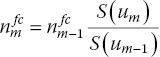
When the population at risk at the beginning of the mth interval is not reported below the KM curve, it can be imputed. First, based on the reported size of the at-risk population at subsequent time points, n m will be estimated according to

With this ‘backward calculation’ approach, we implicitly assume that censoring occurs before the events happen within a time interval. However, this approach is not feasible if there is no information regarding the at-risk population for time intervals, beyond the at-risk population reported at a certain time point. In other words, this approach is only feasibly for intervals up to the latest time point for which an at-risk population is reported. Next, n m will be estimated according to
The disadvantage of this ‘forward calculation’ approach is that censoring is ignored and the sample size potentially too large for those intervals. For intervals where both ![]() and
and ![]() were calculated, the actual estimate for the population at risk is calculated as
were calculated, the actual estimate for the population at risk is calculated as ![]() to ensure the sample size at the beginning of each interval is not overestimated. For intervals where
to ensure the sample size at the beginning of each interval is not overestimated. For intervals where ![]() could not be calculated,
could not be calculated, ![]() .
.
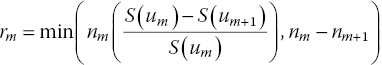
The number of events for each interval is calculated according to
The time intervals do not have to have the same length. In general, the shorter the intervals, the more variation in the hazard function will be picked up, but if the intervals are too short, the number of events will be zero for many subsequent intervals, potentially compromising estimation.
Obviously, the dataset created with the Guyot IPD algorithm can also be used to create interval data, that is, n m and r m for the mth interval.
Appendix D List of RCTs Included in the Illustrative Example in Section 10.10
- 1 Facon, T., Mary, J. Y., Hulin, C., Benboubker, L., Attal, M., Pegourie, B., Renaud, M., Harousseau, J. L., Guillerm, G., Chaleteix, C., Dib, M., Voillat, L., Maisonneuve, H., Troncy, J., Dorvaux, V., Monconduit, M., Martin, C., Casassus, P., Jaubert, J., Jardel, H., Doyen, C., Kolb, B., Anglaret, B., Grosbois, B., Yakoub-Agha, I., Mathiot, C., Avet-Loiseau, H., & Intergroupe Francophone du Myélome. 2007. Melphalan and prednisone plus thalidomide versus melphalan and prednisone alone and reduced-intensity autologous stem cell transplantation in elderly patients with multiple myeloma (IFM 99-06): a randomised trial. Lancet, 370, 1209–1218.
- 2 San Miguel, J. F., Schlag, R., Khuageva, N. K., Dimopoulos, M. A., Shpilberg, O., Kropff, M., Spicka, I., Petrucci, M. T., Palumbo, A., Samoilova, O. S., Dmoszynska, A., Abdulkadyrov, K. M., Schots, R., Jiang, B., Mateos, M. V., Anderson, K. C., Esseltine, D. L., Liu, K., Cakana, A., van de Velde, H., Richardson, P. G., & VISTA Trial Investigators. 2008. Bortezomib plus melphalan and prednisone for initial treatment of multiple myeloma. New England Journal of Medicine, 359, 906–917.
- 3 Hulin, C., Facon, T., Rodon, P., Pegourie, B., Benboubker, L., & Doyen, C. 2009. Efficacy of melphalan and prednisone plus thalidomide in patients older than 75 years with newly diagnosed multiple myeloma: IFM 01/01 trial. Clinical Oncology, 27, 3664–3670.
- 4 Palumbo, A., Bringhen, S., Liberati, A. M., Caravita, T., Falcone, A., Callea, V., Montanaro, M., Ria, R., Capaldi, A., Zambello, R., Benevolo, G., Derudas, D., Dore, F., Cavallo, F., Gay, F., Falco, P., Ciccone, G., Musto, P., Cavo, M., & Boccadoro M. 2008. Oral melphalan, prednisone, and thalidomide in elderly patients with multiple myeloma: updated results of a randomized controlled trial. Blood, 112, 3107–3114.
- 5 Wijermans, P., Schaafsma, M., Termorshuizen, F., Ammerlaan, R., Wittebol, S., Sinnige, H., Zweegman, S., van Marwijk Kooy, M., van der Griend, R., Lokhorst, H., Sonneveld, P., & Dutch-Belgium Cooperative Group HOVON. 2010. Phase III study of the value of thalidomide added to melphalan plus prednisone in elderly patients with newly diagnosed multiple myeloma: the HOVON 49 Study. Journal of Clinical Oncology, 28, 3160–3166.
- 6 Waage, A., Gimsing, P., Fayers, P., Abildgaard, N., Ahlberg, L., & Björkstrand, B. 2010. Melphalan and prednisone plus thalidomide or placebo in elderly patients with multiple myeloma. Blood, 116, 1405–1412.
- 7 Beksac, M., Haznedar, R., Firatli-Tuglular, T., Ozdogu, H., Aydogdu, I., Konuk, N., Sucak, G., Kaygusuz, I., Karakus, S., Kaya, E., Ali, R., Gulbas, Z., Ozet, G., Goker, H., & Undar, L. 2011. Addition of thalidomide to oral melphalan/prednisone in patients with multiple myeloma not eligible for transplantation: results of a randomized trial from the Turkish Myeloma Study Group. European Journal of Haematology, 86, 16–22.
- 8 Owen, R. G., Morgan, G. J., Jackson, H., Davies, F. E., Drayson, M. T., Ross, F. M., Navarro-Coy, N., Gregory, W. M., Szubert, A. J., Rawstron, A. C., Bell, S. E., Heatley, F., & Child, J. A. 2009. MRC Myeloma IX: preliminary results from the non-intensive study. XII International Myeloma Workshop, p. 79. Clinical Lymphoma & Myeloma. DOI: http://dx.doi.org/10.1016/S1557-9190(11)70619-9.
- 9 Mateos, M. V., Oriol, A., Martínez-López, J., Gutiérrez, N., Teruel, A. I., de Paz, R., García-Laraña, J., Bengoechea, E., Martín, A., Mediavilla, J. D., Palomera, L., de Arriba, F., González, Y., Hernández, J. M., Sureda, A., Bello, J. L., Bargay, J., Peñalver, F. J., Ribera, J. M., Martín-Mateos, M. L., García-Sanz, R., Cibeira, M. T., Ramos, M. L., Vidriales, M. B., Paiva, B., Montalbán, M. A., Lahuerta, J. J., Bladé, J., & Miguel, J. F. 2010. Bortezomib, melphalan, and prednisone versus bortezomib, thalidomide, and prednisone as induction therapy followed by maintenance treatment with bortezomib and thalidomide versus bortezomib and prednisone in elderly patients with untreated multiple myeloma: a randomised trial. Lancet Oncology, 11(10), 934–941.