Neutrosophic set in medical image denoising
Mohan Jayaraman*; Krishnaveni Vellingiri†; Yanhui Guo‡ * Department of ECE, SRM Valliammai Engineering College, Kattankulathur, India
† Department of ECE, PSG College of Technology, Coimbatore, India
‡ Department of Computer Science, University of Illinois at Springfield, Springfield, IL, United States
Abstract
Medical computer-aided diagnosis systems are restricted by the presence of noise, uncertainty, and fuzziness in medical images. Such limitations may affect diagnostic decisions while determining the disease type and grade. Fuzzy sets are extensively employed to reduce the uncertainty and fuzziness in several applications; however, such methods ignore the spatial framework of the pixels due to noise. To overcome such limitations of the fuzzy-based methods, the neutrosophic set is used instead. Accordingly, several image denoising approaches were explored based on the neutrosophic theory for interpreting the ambiguity, intrinsic uncertainty, and vagueness, where neutrosophic images are defined by three subsets, namely T, I, and F. This chapter establishes the role of the neutrosophic theory, especially the neutrosophic set (NS), in medical image denoising. The chapter includes mapping an image to the neutrosophic domain for denoising magnetic resonance images (MRI). The NS of median filtering (NS-median), the NS of Wiener filtering (NS-Wiener), and the nonlocal NS of Wiener filtering (NLNS-Wiener) are discussed in detail. The performances of these denoising approaches are evaluated in terms of noise removal and structure preservation by using the Brainweb database of simulated MR images as well as clinical MR images. Moreover, a comparison was conducted with other methods with respect to the quantitative/qualitative measurements. The results illustrated the superiority of the proposed NS-based denoising methods compared to traditional denoising methods, proving the role of the NS for MR image denoising.
Keywords
Medical images; Magnetic resonance images; Rician noise; Wiener filter; Nonlocal mean; Neutrosophic image; Neutrosophic set
1 Introduction
In modern medicine, due to the technological advancements in medical imaging, most clinicians make a diagnosis and provide treatment for a variety of medical conditions based on useful information provided by medical images. The medical conditions include abnormalities in the brain and spinal cord; diseases in the heart, liver, pancreas, and other abdominal organs; injuries or abnormalities in the joints; and abnormalities in various parts of the body. These could be the appearance of features such as tumors or lesions that are abnormally observed, changes in shape such as the shrinkage or enlargement of particular structures, or changes in image intensity compared to normal tissue. In order to achieve the best diagnosis, medical images should be free of noise and artifacts that occur during the acquisition process. Therefore, image denoising is a significant step in medical image analysis to enhance the quality of the images to guarantee precise diagnosis.
Among different medical imaging modalities, MRI is a notable medical imaging technique for comprehensively visualizing the human body's internal structure, where the nuclei in a magnetic field absorbs and reemits electromagnetic radiation. MRI has numerous applications in medicine, material science, and engineering. In clinical practices, MRI is used primarily to determine pathological/physiological changes of human tissues (Wright, 1997). In MRI, the image is formed by measuring the signal coming from certain protons/nuclei in a subject using the interaction between the nuclear spin and the electromagnetic field (Wright, 1997). Nuclear spin is a fundamental property of protons and neutrons. Each unpaired proton and neutron possesses the value of nuclear spin = 1/2, which is commonly used for NMR. Only incompletely paired nuclei, which possess an odd number of protons and/or neutrons, have net spins that induce magnetic moments. Hydrogen is one such element with an uncancelled (unpaired) spin. The hydrogen nuclei spin around their axes as small magnets. Mainly, the human body includes water molecules and fat. Usually, the hydrogen protons in the water molecules are imaged to show the human tissues’ pathological/physiological changes (Rummeny, Reimer, & Heindel, 2009).
MRI scanners produce a strong stationary magnetic field. In current clinical practice, the field strength varies from 0.5 to 3 T. For research purposes, magnets with the strength of 7 T or 11 T and above are also used. When an individual is placed in the static magnetic field, the hydrogen atoms with a spin will tend to align themselves along the direction of the magnetic field, a process called magnetization. These protons process around the direction of the magnetic field with a frequency proportional to the static magnetic field, called the Larmor frequency. For hydrogen nuclei in a typical 1.5 T field, the Larmor frequency is approximately 64 MHz (Rummeny et al., 2009). The average magnetization of the protons along the magnetic field direction is known as the longitudinal net magnetization. At the Larmor frequency, a brief radiofrequency (RF) pulse is applied to make the protons absorb energy, brought out of equilibrium and the longitudinal magnetization flipped into the transverse plane to produce transverse magnetization, which is called excitation. When the RF pulse ends, the protons will return to equilibrium by reemitting the energy absorbed, which is called relaxation. This reemitting energy by the protons is observed as MR signals. The MRI system detects this signal for further image reconstruction, where the phase and frequency of the signal data are gathered in the k-space, which is the abstract platform used to position the acquired data (Rodriguez, 2004). Then, for this k-space, a two-dimensional (2D) inverse Fourier transform is calculated to create a gray-scale image.
During the acquisition process, random noise affects the MR, which degrades the diagnosis using the acquired MRI images and affects the performance of any further image analysis procedures. The typical noise type that affects the magnitude of MR images follows Rician distribution, which is signal-dependent (Gudbjartsson & Patz, 1995). Particularly, Rician noise introduces random fluctuations/bias, the removal of which is a challenging task. Therefore, denoising is used as a preprocessing stage prior to several image-processing procedures to enhance the MR image quality for precise diagnosis. Accordingly, several researchers were interested to implement different denoising approaches to reduce the Rician noise on MR images by different assumptions, merits, and demerits (Anand & Sahambi, 2010; Coupe et al., 2008; He & Greenshields, 2009; Manjon et al., 2008; Nowak, 1999; Rajan, Jeurissen, Verhoye, Audekerke, & Sijbers, 2011). Generally, efficient denoising techniques have to remove noise while preserving the image anatomical structures. However, this is considered a challenging problem in MR image denoising, owing to the trade-off problem between noise removal and preserving the significant features. To resolve this challenging task, the neutrosophic theory can be used, where neutrosophy is the root of neutrosophic logic that generalizes the classical/fuzzy set. In addition, it is considered the base of the neutrosophic probability that generalizes the classical probability.
Neutrosophy defines knowledge fuzziness and inaccuracy in the data, such as the images (Smarandache, 2003). For images, noise is considered a type of indeterminant information. Thus, the NS can be efficiently applied to noisy images during the denoising process to achieve superior performance. Therefore, in this chapter, new methodologies for denoising MR images based on the NS theory to realize a balance between noise reduction and structure conservation are discussed.
2 Noise in MR images
In MR image acquisition, the noise still pretentious the images’ visual quality even if the MR scanners has endured remarkable developments in speed of acquisition, spatial resolution, and signal to noise ratio (SNR). Typically, an MRI contains varying noise amounts from different sources, such as the noise from the eddy currents, physiological processes, stochastic variation, and rigid/nonrigid body motion (Redpath, 1998; Zhu et al., 2009). The thermal noise is considered the major noise source in the MR images, and it is produced from the MR scanners that affects the scanned objects. Generally, the thermal noise's variance is considered the sum of the variance from stochastic processes that represent the electronics, coils in the MR scanners, and the patient's body (Macovski, 1996). These noise sources degrade the MR images’ acquisition and the measurements from the acquired data. For example, tissue characteristics, the radio-frequency (RF) coil, pulse sequence, static field intensity, voxel size, and the receiver bandwidth all affect the SNR. As follows, the noise characteristics in MR images are introduced.
For a single coil acquisition during the MRI scanning process, the obtained raw data are complex numbers that denote the Fourier transform (FT) result on the magnetization scattering in a volumetric tissue at a specific time (Kuperman, 2000). These raw data are then converted into magnitude, phase, and frequency components using the inverse FT to characterize the morphological and physiological features of the region of interest in the scanned organ (Wright, 1997; Zhu et al., 2009). Consequently, in the k-space, the noise is presumed to have a Gaussian distribution with the same variance on real and imaginary components due to the FT linear and orthogonal properties (Edelstein, Bottomley, & Pfeifer, 1984; Gudbjartsson & Patz, 1995; Henkelman, 1985). Thus, the PDF (probability density function) changes for the acquired data. In the spatial domain, the data magnitude has a Rician model distribution, and the error between the intensity of the original and the measured data is called Rician noise (Gudbjartsson & Patz, 1995).
Typically, the complex Gaussian process is used to model the complex spatial MR data. Thus, this complex spatial signal can be formulated as:
where A represent the noiseless original signal and the complex uncorrelated Gaussian noise is n(σn2) = nr(X; σn2) + jni(X; σn2) that has zero mean and σn2 noise variance. Hence, the magnitude of the complex signal represents the Rician distributed envelope, which is given by (Aja-Fernandez, Tristan-Vega, & Alberola-Lopez, 2009; Gudbjartsson & Patz, 1995):
Additionally, the PDF can be expressed as follows:
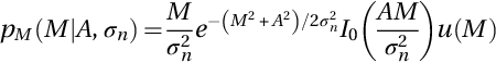
where I0(⋅) represents the adapted zeroth-order Bessel function, u(⋅) the Heaviside step function, and M is a variable representing the MR magnitude. Typically, the Rician distribution in high SNR tends to be equivalent to a Gaussian distribution with ![]() mean and σn2 variance as follows:
mean and σn2 variance as follows:
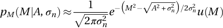
However, with zero SNR in the image background, the Rician PDF can be represented as a Rayleigh distribution that has PDF that can be formulated as follows (Aja-Fernandez et al., 2009; Gudbjartsson & Patz, 1995):

Generally, in the low SNR ranges, the Rician noise is problematic as it introduces a signal-dependent bias. During denoising the squared MR images, the bias remains as a constant term 2σn2, which can be removed easily (Manjon et al., 2008; Nowak, 1999) by subtracting the bias term from the noisy image as follows:
The postprocessing noise reduction techniques are applied to guarantee the high-quality MR image, which is of extreme importance in a more accurate diagnosis.
The noise-driven anisotropic diffusion filter for removing Rician noise from MR images was introduced by Krissian and Aja-Fernández (2009). In this filter, parameters are selected automatically from the estimated noise. The diffusion filter's convergence rate can be improved by combining the linear, planar, and volumetric components of the local image structure while conserving contours to guarantee an intuitive and robust filtering process. Zhang and Ma (2010) proposed the anisotropic coupled diffusion equation-based MR image denoising method. In the coupled partial diffusion equations, one equation consists of a diffusion direction controlling term (anisotropic diffusion term), the assurance of the correlation between the filtered image and the initial image (fidelity term), and controlling the diffusion speed of each pixel (diffusion gene). Therefore, this method offers acceptable noise reduction with detail protection ability in the denoised MR images.
Coupe, Yger, and Barillot (2006) proposed a three-dimensional (3D) MR image denoising method by using optimized (multithreading) implementation of the nonlocal mean (NLM) filter. The computational time of the filter is considerably decreased up to 50 times. They later extended this work with fully automated blockwise implementation of an NLM filter (Coupe et al., 2008) for denoising 3D MR images. This is achieved by tuning the smoothing parameter automatically; the NL means was computed by selecting the utmost significant voxels, blockwise implementation, and parallelized computation. By using this approach, the computational time is reduced up to 60 times compared to the original NLM filter. The dynamic nonlocal means (DNLM) denoising method was introduced by Gal et al. (2009) for denoising the dynamic contrast enhanced MR images. This method is implemented as a variation of the NLM algorithm by exploiting information redundancy in different volumes of images that are acquired at different time intervals. In 3D MR images, an improved NLM filter with preprocessing (PENLM) was proposed to remove the Rician noise by Liu, Udupa, Odhner, Hackney, and Moonis (2005). In this method, first, the squared magnitude image gets denoised by the NLM filter, and then bias deviation is removed by performing the unbiased correction. The weight of the NLM filter is considered based on the Gaussian-filtered image in order to decrease the noise disturbance. For 3D MR image denoising, Manjon, Coupe, Buades, Collins, and Robles (2012) introduced a denoising method that exploits the self-similarity and sparseness properties of the images. For denoising the same types of image, Coupe, Manjon, Robles, and Collins (2012) proposed an adaptive multiresolution of the blockwise nonlocal means filter. This filter uses the spatial and frequency information in the image to adapt the amount of denoising by using an adaptive soft wavelet coefficient mixing to enhance the NLM filter performance.
In all these MR image denoising methods, there are computational burdens due to the calculation complexity of the pixel/voxel weight. In this chapter, the NS-based MR image denoising method was used to achieve a balance between noise reduction and structure preservation with reduced computational complexity.
3 Neutrosophic set-based MR image denoising
For NS-based MR image denoising, the noisy MR image is transferred to the NS domain that is defined by true, indeterminacy, and false subsets, which are symbolized as T, I, and F, respectively. The entropy is used to measure its indeterminacy. In the present work, the filtering operator is performed on T and F to reduce the indeterminacy set and obtain the denoised image, as illustrated in Fig. 1.

In this chapter, three NS-based MR image denoising methods, including the NS of γ-median filtering (NS-median) (Mohan, Krishnaveni, & Guo, 2011), the NS of ω-Wiener filtering (NS-Wiener) (Mohan, Krishnaveni, & Guo, 2013a), and the nonlocal NS of ω-Wiener filtering (NLNS-Wiener) (Mohan, Krishnaveni, & Guo, 2013b), were introduced.
3.1 Neutrosophic image
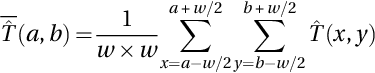
The noisy MR image is mapped into NS space, where the NS image HNS is defined by T, I, and F. A pixel H(a, b) in an image is mapped into the NS domain, HNS(a, b) = {T(a, b), I(a, b), F(a, b)}, where T(a, b), I(a, b), and F(a, b) are the true, indeterminate, and false sets, respectively (Guo, Cheng, & Zhang, 2009), which are represented for an image G as:

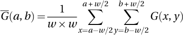

where the pixels in the window have ![]() local mean, and δ(a, b) denotes the absolute value of the difference between intensity G(a, b) and its
local mean, and δ(a, b) denotes the absolute value of the difference between intensity G(a, b) and its ![]() .
.
For a gray-scale image, the entropy is calculated to assess the gray level distribution. Maximum entropy occurs when the intensities have equal probability with uniform distribution. Small entropy occurs with the intensities having different probabilities with nonuniform distribution. The entropy in the neutrosophic image is considered the totality of the T, I, and F entropies, which is used to measure the element distribution in the NS domain (Guo et al., 2009); that is expressed as:


where the entropies are EnT, EnI, and EnF for T, I, and F respectively. Furthermore, the probabilities of the element k are pT(k), pI(k), and pF(k) in T, I, and F, respectively. The I(a, b) value is engaged to calculate the indeterminacy of element HNS(a, b). To produce the correlated T and F with I, the changes in T and F effect the element distribution in I and the entropy of I. The general flowchart for NS-based denoising of MR images is shown in Fig. 2.

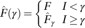
3.2 Neutrosophic set method of γ-median filtering
As discussed in the above section, the MR image is mapped into the T, I, and F sets. The I(a, b) values are used to calculate the indeterminate of HNS(a, b). To generate the correlated set I with T and F, the variations in T and F effect the element spreading in I and change the entropy of I. A γ-median filter operator named ![]() is denoted as (Guo et al., 2009):
is denoted as (Guo et al., 2009):


where at the location (a, b), the absolute value ![]() of the difference between the intensity
of the difference between the intensity ![]() and its local mean
and its local mean ![]() after the γ-median filter operator is used.
after the γ-median filter operator is used.
For MR image denoising, the NS-based median filtering is listed as follows:
- 1. Map the MR image in the NS domain.
- 2. Apply the γ-median filter operator on T to obtain
 .
. - 3. Calculate the entropy of
 .
. - 4. Go to step 5, if
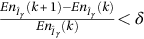 ; Else
  , go to 2.
 - 5. Transform from the NS domain to the gray level.
There are two methods to improve the NS median MR image denoising method's performance (Mohan et al., 2011). One method is to apply the new filtering method instead of the median filter on T and F to reduce the indeterminacy. Hence, the NS Wiener technique is proposed for MR image denoising of uniformly distributed Rician noise (Mohan et al., 2013a). On the other side, in the second technique, the noisy MR image is prefiltered by using the NLM algorithm to reduce the noise before transforming the noisy image to the NS domain, and then the filtered image is used for further noise reduction in the NS domain. Hence, the NLNS Wiener technique is proposed for MR image denoising of uniformly distributed Rician noise (Mohan et al., 2013b).
3.3 Neutrosophic set method of ω-Wiener filter
Similar to the preceding methods, the MR image is converted first to the NS space as T, I, and F subsets. I(a, b) is used to calculate the indeterminate degree of element HNS(a, b). A ω-Wiener filter operator for HNS, ![]() is expressed as:
is expressed as:


where ![]() is the absolute number of the difference between the intensity
is the absolute number of the difference between the intensity ![]() and its local mean value
and its local mean value ![]() at (a, b) after the ω-Wiener filter operator.
at (a, b) after the ω-Wiener filter operator.
The MR image NS-based denoising technique using the Wiener filter is given as:
- 1. Map the image in the NS domain.
- 2. Apply the ω-Wiener filter operator on T to obtain
 .
. - 3. Calculate the entropy of
 .
. - 4. Go to step 5, if
 , else
  , go to Step 2.
 - 5. Convert from the NS back to the image domain.
3.4 Nonlocal neutrosophic set method of ω-Wiener filter
The noisy MR image is filtered by using the NLM algorithm to improve the denoising method performance. In this procedure, a nonlocal means (NLM) operation is applied. The NLM technique is used on the noisy MR images to produce a reference image. In the image, assume a noisy image u = {u(a)| a ∈ I}, thus by applying the nonlocal mean (Buades, Coll, & Morel, 2005), the estimated value NL[u](a) for a pixel a can be calculated as a weighted average as follows:

where the weights set {w(a, b)}b depends on the likeness between the pixels a and b, and fulfills the constraints 0 ≤ w(a, b) ≤ 1 and ∑bw(a, b) = 1. This similarity is related to the likeness of the intensity vectors u(Na) and u(Nb), where Nc is the neighborhood centered at a pixel c. This similarity is calculated as a reducing function of the weighted Euclidean distance, ‖u(Na) − u(Nb)‖2, σ2, where σ > 0 is the Gaussian kernel's standard deviation. Using the Euclidean distance to the noisy neighborhoods increases the succeeding equality:
After calculating the Euclidean distance between the vectors, the weight of the pixel is assigned as follows:

where Z(a) is the normalization constant as:

In addition, h is considered a filtering degree that controls the exponential function decay, and hence the weights decay is related to the Euclidean distances.
After prefiltering on the noisy MR image, the NLM prefiltered image is mapped to the NS domain, the entropy is computed, and a ω-Wiener filtering operation is performed on T and F in order to reduce the indeterminacy; hence, the noise is removed from the image. The Rician noise characteristics are adopted by estimating the σ of the noise from the noisy MR image using the local skewness estimation of the magnitude data distribution (Rajan, Poot, Juntu, & Sijbers, 2010). The bias is reduced by subtracting 2σ2 from the squared denoised image, as discussed by Nowak (Nowak, 1999). The summary of the NLNS-based Wiener filter MR image denoising is given by:
- 1. Apply the NLM algorithm to the noisy MR image.
- 2. Map the NLM filtered image in the NS domain.
- 3. Apply the ω-Wiener filter on the T to obtain Tω.
- 4. Calculate the entropy of .
- 5. Go to step 6, if , else , go to Step 3.
- 6. Convert from the NS domain to the gray-level domain.
4 Performance evaluation metrics of NS-based denoising of MR image
The effectiveness of the denoising procedures can be evaluated using metrics used for assessing the MR image denoising method performance. For quantitative assessment, the PSNR, the mean absolute difference (MAD), the structural similarity (SSIM) index (Wang, Bovik, Sheikh, & Simoncell, 2004), and the Bhattacharyya coefficient (BC) (Bhattacharyya, 1943) are evaluated. Generally, PSNR is used as the quality measure because it can be simply calculated. But, according to Wang et al. (2004), another objective quality measure is the SSIM, which depends on the structural content of the image. The BC values depend on the image histogram that shows the similarity between the original and denoised images. MAD is used for measuring the dispersion of the data. Along with PSNR, SSIM, BC, and MAD are also adopted as quantitative metrics. According to Rajan et al. (2011), an MRI denoising method is effective and good when it gives a higher value of PSNR, SSIM, and BC and a lower value of MAD.
4.1 Peak signal-to-noise ratio
The PSNR is an independent quality that measures the estimated value deviation from the true value in decibels (dB). It can be measured as follows:

where H × W is the image's size, and S(a, b), and Sd(a, b) are the pixel (a, b) intensities in the original and denoised images, respectively.
4.2 Structural similarity index
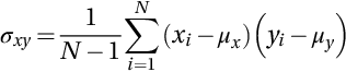
The PSNR cannot be considered as optimal in terms of the perceived quality (Wang et al., 2004). However, the SSIM is considered an efficient alternative to improve the error measures, which is reliable to the visual perception. It measures the similarity in structure between the original and denoised images and is in [0, 1]. Let x and y be two nonnegative images, where one of them has perfect quality. Thus, the SSIM can be used to measure the similarity of the second image using the following formula:

where C1 and C2 are constants, which can be given by C1 = (K1L)2, and C2 = (K2L)2 as K1, K2 < < 1 is a small constant and L is the dynamic range of the pixel values. In addition, μx and μy are the estimated mean intensity, and σx and σy are the standard deviations, respectively, where σxy is given by:
4.3 Bhattacharyya coefficient
The BC is a correlation metric that determines the statistical similarity between two images. It measures the closeness between two image histograms. The distances between the histogram of the denoised image and that of the original image are estimated by BC, which is given by (Bhattacharyya, 1943):
where m and n are the two histograms. The range of BC is 0 to 1, where a closer BC value to 1 specifies similar histograms of m and n.
4.4 Mean absolute difference
The MAD is the absolute deviation mean value of a set of data about the data's mean. It is a better choice for measuring the dispersion of the data. The MAD for a dataset {xi} is calculated using the following expression:
4.5 Residual image
The residual image is obtained by deducting the denoised image from the noisy one (Manjon et al., 2008). It is calculated to prove the traces of anatomical information that are detached in the denoising process. Henceforth, it discloses the extreme smoothening and blurring of small details that exist in an image.
5 MRI dataset
The experiments are applied on two MRI datasets, namely a simulated MR Brainweb database (Kwan, Evans, & Pike, 1999) and a clinical dataset. The simulated MR image dataset consists of a T1/T2 weighted axial, a PD weighted axial, a T1/T2 weighted axial with a multiple sclerosis (MS) lesion, and a PD weighted axial with MS lesion volumes of 181 × 217 × 181 voxels and a voxel resolution of 1 mm3. They are degraded by different degrees of Rician noise (1%–15% of maximum intensity) (Manjon, Coupe, Marti-Bonmati, Collins, & Robles, 2010). The MS is a neurological disease that may be observed as small plates in the brain MR images. In the complex domain, the Rician noise is created from white Gaussian noise. First, the real and imaginary images are calculated as:
where S0 is the original image and σ is the standard deviation of the added white Gaussian noise. Thus, the noisy image can be considered as:
The squared magnitude image has a signal independent noise bias that can be easily removed (Rajan et al., 2010). Another dataset includes a clinical MRI from the PSG Institute of Medical Sciences and Research (PSG IMS & R), Coimbatore, Tamilnadu, India. This dataset consists of more than 70 patients with different age groups; both male and female images were acquired using a Siemens Magnetom Avanto 1.5T Scanner. It contains T1 weighted and T2 weighted axials as well as coronal and sagittal images with 5 mm thickness and 512 × 512 pixels.
6 Results and discussion
The performance of the NS median, the NS Wiener, and the NLNS Wiener methods was compared with different standard procedures, such as the nonlocal maximum likelihood (NLML) method (He & Greenshields, 2009), the restricted local maximum likelihood (RLML) method (Rajan et al., 2011), the nonlocal mean (NLM) filter (Buades et al., 2005), the total variation (TV) minimization scheme (Rudin, Osher, & Fatemi, 1992), the Wiener filter, and anisotropic diffusion (AD) (Perona & Malik, 1990). In the present chapter, the setting of the parameters of the NLML method is as follows: the window size m = 11 and neighborhood size n = 3 and k = 25 (He & Greenshields, 2009). For the RLML filter, the neighborhood window size for denoising is assumed to be 7 × 7 × 3 and the neighborhood size for local computation range 3 × 3 × 3 (Rajan et al., 2011). For the NLM filter, there are three main parameters, namely the search window (w) size, the neighborhood window (f) size, and the filtering (h) degree. In this chapter, these parameter settings are chosen as w = 5 and f = 2 while h is proportional to the noise level of the image (Gal et al., 2009). For TV minimization, a range from 0.01 to 1 is used for the parameter λ with a step of 0.01, and the number of iterations varies from 1 to 10 (Coupe et al., 2008). In the AD filter, the used parameter K ranges from 0.05 to 1 with a step of 0.05 and the number of iterations from 1 to 15.
The PSNR, SSIM, BC, and MAD obtained for the T1 weighted MR images with different noise degrees (1%–15%) using the Wiener, TV, ADF, NLM, NLML, RLML, NS median, NS Wiener, and the NLNS Wiener denoising techniques are depicted in Fig. 3. From the PSNR value presented in Fig. 3A, it is clear that the NLNS Wiener filter produces good PSNR values compared with the Wiener, TV, ADF, NLM, NLML, RLML, NS median, and NS Wiener methods for all noise levels. The NLNS Wiener filter gives an average PSNR gain of 7.81, 7.01, 8.66, 6.15, 5.59, 5.06, 5.52, and 1.86 dB compared to Wiener, TV, ADF, NLM, NLML, RLML, NS median, and NS Wiener methods, respectively. In Fig. 3B, the SSIM value gives the similarity measures between the original image and the denoised image. Compared to the Wiener, TV, ADF, NLM, NLML, RLML, NS median, and NS Wiener methods, the SSIM value of the NLNS Wiener filter is measured an average of 5.12%, 4.48%, 3.57%, 3.42%, 3.06%, 2.02%, 1.36%, and 0.15% higher values, respectively, for all noise levels. This higher value of SSIM shows that the NLNS Wiener filter outperforms the other techniques.

The statistical similarity measure BC value is plotted in Fig. 3C. Compared to the Wiener, TV, ADF, NLM, NLML, RLML, NS median, and NS Wiener methods, the NLNS Wiener filter has produced an average of 6.97%, 6.6%, 7.3%, 5.8%, 3.8%, 3.22%, 3.1%, and 1.82% higher BC values, respectively. This higher value of BC ensures that the denoised image produced by the NLNS Wiener filter has strong correlation with the original image. In Fig. 3D, the MAD value for different levels of noise is plotted. The MAD value for the NLNS Wiener filter is measured an average of 2.89, 2.81, 3, 2.4, 2.19, 1.82, 1.75, and 0.34 lower values, respectively, compared to the Wiener, TV, ADF, NLM, NLML, RLML, NS median, and NS Wiener methods. The lower value of MAD shows that the NLNS Wiener filter outperforms the other techniques.
The qualitative comparison of the NS median, NS Wiener, and NLNS Wiener methods on a pathological case is shown in Fig. 4. To enable visual analysis, the magnification of the part of the image is shown in Fig. 4. In this analysis, three continuous slices of T2 weighted MR images with MS lesions (slice numbers 104, 105, and 106) from the Brainweb database with 15% Rician noise are used. In Fig. 4A, the original images of the T2 weighted slices 104, 105, and 106 are shown. The magnified version of the original and noisy images with 15% Rician noise for the white rectangle marked region is shown in Fig. 4B and C. The denoised result of the NS median, NS Wiener, and NLNS Wiener methods are shown in Fig. 4D–F. From these images, it can be perceived that the NLNS Wiener method maintains visually better MS lesions compared to the NS median and NS Wiener methods.
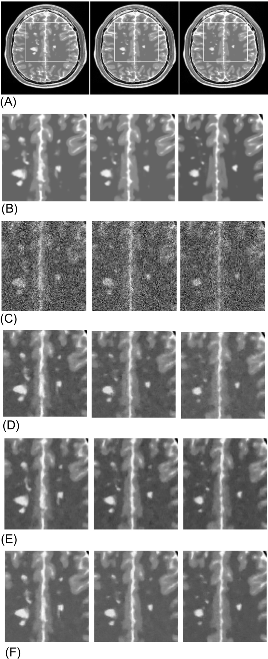
Table 1 reports the comparison results using the different denoising techniques based on the quantitative parameters. Generally, the higher the values of PSNR, SSIM, and BC, the lower the value of MAD, showing the superiority of NS-based MR image denoising methods compared to the other denoising approaches.
Table 1
| MR image | Methods | Metrics | |||
|---|---|---|---|---|---|
| PSNR (dB) | SSIM | BC | MAD | ||
| PD-weighted brain MRI with MS lesions corrupted by 7% Rician noise | Wiener | 24.42 | 0.9427 | 0.835 | 7.2 |
| TV | 24.54 | 0.9545 | 0.84 | 7.5 | |
| ADF | 25.37 | 0.9642 | 0.832 | 7.12 | |
| NLM | 25.36 | 0.9647 | 0.85 | 6.52 | |
| NLML | 26.52 | 0.9694 | 0.876 | 6.45 | |
| RLML | 26.62 | 0.9734 | 0.883 | 6.4 | |
| NS Median | 27.19 | 0.9787 | 0.89 | 6.18 | |
| NS Wiener | 29.5 | 0.9889 | 0.9 | 4.52 | |
| NLNS Wiener | 31.37 | 0.9895 | 0.902 | 4.18 | |
| T2 weighted brain MRI with MS lesions corrupted by 9% Rician noise | Wiener | 22.12 | 0.8337 | 0.82 | 10.06 |
| TV | 22.59 | 0.9345 | 0.809 | 9.92 | |
| ADF | 22.67 | 0.9466 | 0.816 | 10.09 | |
| NLM | 23.39 | 0.9495 | 0.823 | 8.86 | |
| NLML | 23.75 | 0.9512 | 0.835 | 8.73 | |
| RLML | 23.96 | 0.9594 | 0.843 | 8.36 | |
| NS Median | 24.4 | 0.9696 | 0.85 | 8.28 | |
| NS Wiener | 26.19 | 0.9887 | 0.86 | 6.39 | |
| NLNS Wiener | 27.24 | 0.9816 | 0.88 | 5.65 | |
| T1 weighted brain MRI with MS lesions corrupted by 15% Rician noise | Wiener | 16.78 | 0.7870 | 0.808 | 13.71 |
| TV | 16.82 | 0.7901 | 0.809 | 13.69 | |
| ADF | 16.84 | 0.8127 | 0.806 | 13.74 | |
| NLM | 16.88 | 0.8370 | 0.83 | 13.241 | |
| NLML | 18.96 | 0.8426 | 0.836 | 12.87 | |
| RLML | 19.22 | 0.8842 | 0.841 | 12.21 | |
| NS Median | 20.51 | 0.9062 | 0.846 | 11.657 | |
| NS Wiener | 23.53 | 0.9263 | 0.855 | 9.17 | |
| NLNS Wiener | 25.23 | 0.9284 | 0.867 | 8.65 | |

In the clinical data, denoising results obtained for the T2 weighted Sagittal MR image of a normal brain with TR = 4460 ms, TE = 85 ms, 5 mm thickness, and 512 × 512 resolution are illustrated in Fig. 5. In Fig. 5A, the original image is shown. The denoised images of the Wiener, TV, ADF, and NLM methods are demonstrated in Fig. 5B–F, respectively. Moreover, the residual images are shown in Fig. 5C–J, respectively. From these images, it is clear that there are more traces of anatomical structures in the residual images. Even though the NLML and RLML methods produce good denoised images as shown in Fig. 5G and L, there are fewer traces of anatomical structures present in the residual images (Fig. 5K and P). The NS median, NS Wiener, and NLNS Wiener methods give detailed information and the edges in the denoised images are kept, as shown in Fig. 5M–O. While comparing the residual images as shown in Fig. 5Q–S, it is seen that the NLNS Wiener approach is superior to the NS median and NLNS Wiener methods.

In the Wiener, TV, ADF, NLM, NLML, and RLML methods for denoising MR images, the filtering operation is performed directly in the noisy MR image. In the NS-based MR image denoising methods, the noisy MR image is characterized by T, I, and F membership sets in the NS domain. The entropy of the NS evaluates the indeterminacy. The filtering operation has been performed on T and F to reduce the indeterminacy and the denoised image is obtained. Therefore, from the quantitative and qualitative evaluation of the MR image denoising methods on the Brainweb database and the clinical MRI dataset, it is clear that the NS-based MR image denoising methods such as NS median, NS Wiener, and NLNS Wiener outperform the other state-of-the-art studies, such as the Wiener, TV, ADF, NLM, NLML, and RLML methods.
7 Conclusions
In this chapter, the neutrosophic approach of MR image denoising methods such as NS median, NS Wiener, and NLNS Wiener are discussed for denoising MR images with uniform Rician noise. Numerous validations were performed with both synthetic and clinical MR images. The performances are analyzed based on the noise removal and structure preservation and compared with Wiener, TV, ADF, NLM, NLML, and RLML. For noise removal, the quantitative metrics such as PSNR, SSIM, BC, and MAD are used. As for the Wiener, TV, ADF, NLM, NLML, and RLML, the NS-based filters (NS median, NS Wiener, and NLNS Wiener) are able to restore images degraded by Rician noise. Also, experiments demonstrated that the NLNS Wiener filtering method can remove noise efficiently with different degrees of noise compared to the NS median filter and the NS Wiener filter.
Validation on the structure-preservation ability of the NS-based denoising methods is done by comparing the denoised image with its original noise-free image and by visual inspection of the residual image. It is found that the denoised image of the NLNS Wiener method has high correlation with the original image. And also, for high noise level, the traces of anatomical structures in the residual images are seen less often compared to that of the Wiener, TV, ADF, NLM, NLML, RLML, NS median, and NS Wiener methods. The preservation of the fine structural details such as pathological signatures is explained with the experimental results of T2 weighted MR images with MS lesions of three continuous slices (slices 104, 105, and 106). From the results, the NLNS Wiener technique displayed better performance over the NS median and NS Wiener methods in preserving the given pathology and removing the noise.