
Data ingestion is the process of transferring, loading, and processing data into a data management or storage platform. This chapter discusses various tools and methods on how to ingest data into Kudu in batch and real time. I’ll cover native tools that come with popular Hadoop distributions. I’ll show examples on how to use Spark to ingest data to Kudu using the Data Source API, as well as the Kudu client APIs in Java, Python, and C++. There is a group of next-generation commercial data ingestion tools that provide native Kudu support. Internet of Things (IoT) is also a hot topic. I’ll discuss all of them in detail in this chapter starting with StreamSets.
StreamSets Data Collector
StreamSets Data Collector is a powerful, enterprise-grade streaming platform that you can use to ingest, route, and process real-time streaming and batch data from a large variety of sources. StreamSets was founded by Girish Pancha, Informatica’s ex-chief product officer; and Arvind Prabhakar, an early employee of Cloudera, where he led the development of Apache Flume and Apache Sqoop. i StreamSets is used by companies such as CBS Interactive, Cox Automotive, and Vodafone. ii
Data Collector can perform all kinds of data enrichment, transformation, and cleansing in-stream, then write your data to a large number of destinations such as HDFS, Solr, Kafka, or Kudu, all without writing a single line of code. For more complex data processing, you can write code in one of the following supported languages and frameworks: Java, JavaScript, Jython (Python), Groovy, Java Expression Language (EL), and Spark. Data Collector can run in stand-alone or cluster mode to support the largest environments.
Pipelines
To ingest data, Data Collector requires that you design a pipeline. A pipeline consists of multiple stages that you configure to define your data sources (origins), any data transformation or routing needed (processors), and where you want to write your data (destinations).
After designing your pipeline, you can start it, and it will immediately start ingesting data. Data Collector will sit on standby and quietly wait for data to arrive at all times until you stop the pipeline. You can monitor Data Collector by inspecting data as it is being ingested or by viewing real-time metrics about your pipelines.
Origins
In a StreamSets pipeline, data sources are called Origins. They’re configurable components that you can add to your canvas without any coding. StreamSets includes several origins to save you development time and efforts. Some of the available origins include MQTT Subscriber, Directory, File tail, HDFS, S3, MongoDB, Kafka, RabbitMQ, MySQL binary blog, and SQL Server and Oracle CDC client to name a few. Visit StreamSets.com for a complete list of supported origins.
Processors
Processors allows you to perform data transformation on your data. Some of the available processors are Field Hasher, Field Masker, Expression Evaluator, Record Deduplicator, JSON Parser, XML Parser, and JDBC Lookup to name a few. Some processors, such as the Stream Selector, let you easily route data based on conditions. In addition, you can use evaluators that can process data based on custom code. Supported languages and frameworks include JavaScript, Groovy, Jython, and Spark. Visit StreamSets.com for a complete list of supported processors.
Destinations
Destinations are the target destination of your pipeline. Available destinations include Kudu, S3, Azure Data Lake Store, Solr, Kafka, JDBC Producer, Elasticsearch, Cassandra, HBase, MQTT Publisher, and HDFS to name a few. Visit StreamSets.com for a complete list of supported destinations.
Executors
Executors allow you to run tasks such as a MapReduce job, Hive query, Shell script, or Spark application when it receives an event.
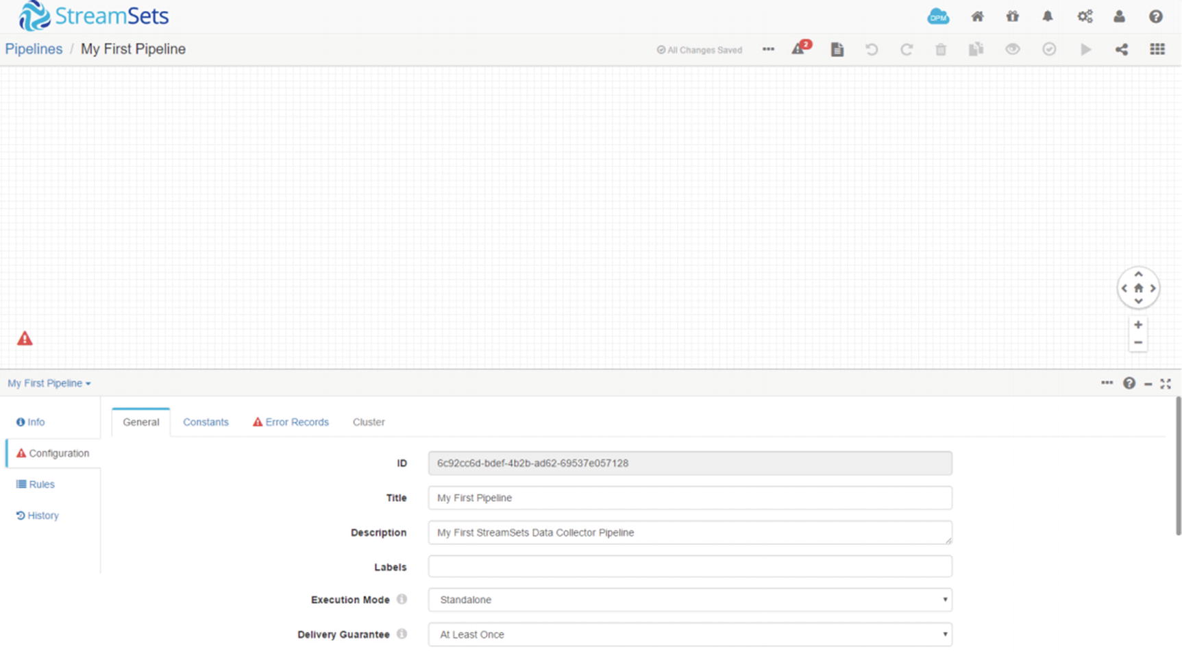
Data Collector Console
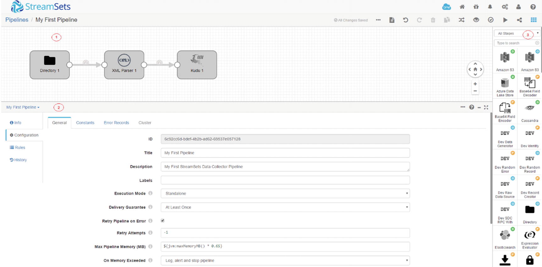
StreamSets Data Collector console
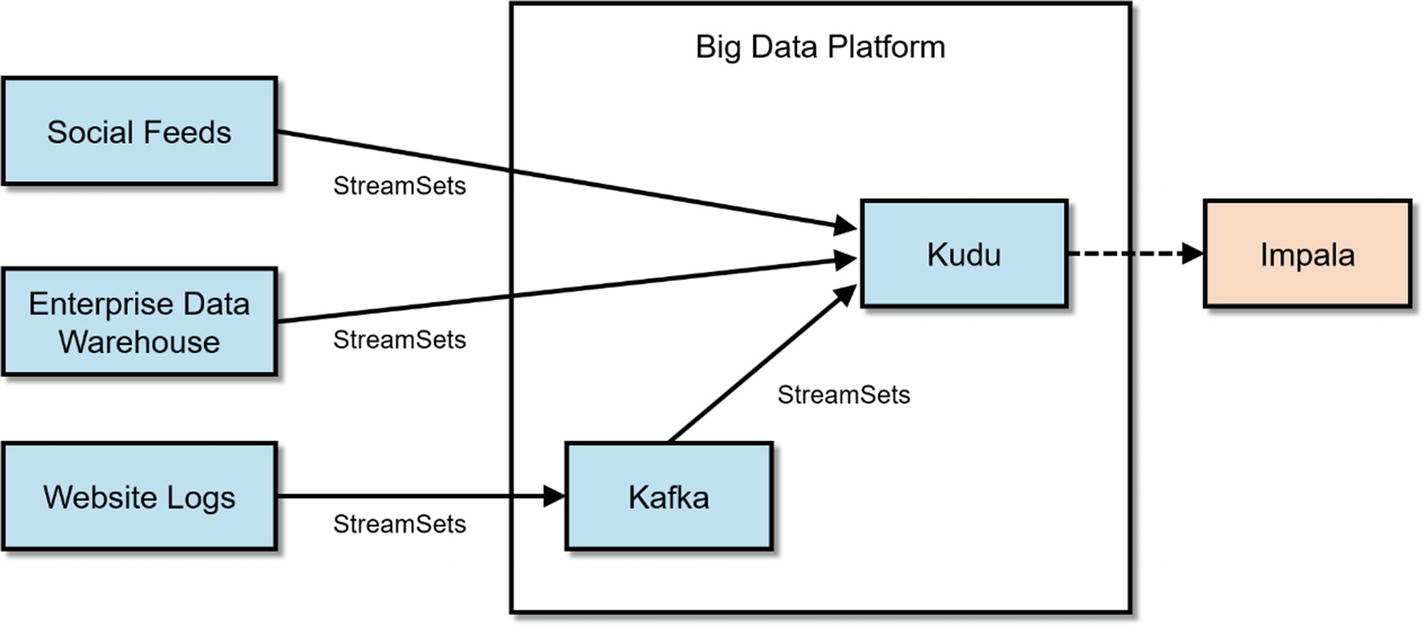
Typical StreamSets Architecture
There are several pre-built processors for some of the most common data transformations and enrichments. Examples of processors include column splitters and hashers, data type converters, XML parsers, JDBC lookups, and Stream processors to name a few. These processors can be configured without writing a single line of code. However, there are times when you want to write code, mainly, because none of the existing processors can handle the specific type of transformation that you require. StreamSets provide evaluators that support JavaScript, Java, Java EL, Spark, Jython, and Groovy. StreamSets connects all these stages (origins, processors, data sources) to form a pipeline. StreamSets executes the pipeline in-memory, providing maximum performance and scalability.
Real-Time Streaming
As discussed in previous chapters, Kudu is especially suitable for real-time ingestion and processing because of its support for efficient inserts and updates as well as fast columnar data scans. iii For real-time workloads, users need to select the right type of destination. There are storage engines that are not designed for real-time streaming. Examples of these storage engine includes HDFS and S3.
HDFS was designed for batch-oriented workloads. It splits and writes data in 128MB block sizes (configurable) to enable high throughput parallel processing. The problem arises when real-time data ingestion tools such as StreamSets or Flume start writing data to HDFS as fast as it receives them in order to make the data available to users in real time or near real time. This will cause HDFS to produce tons of small files. As mentioned earlier, HDFS was not designed to handle small files. iv Each file, directory, or block in HDFS has metadata stored in the name node’s memory. Sooner or later, the amount of memory consumed by these small files will overwhelm the name node. Another problem with small files is that they are physically inefficient to access. Applications need to perform more IO than necessary to read small files. A common workaround is to use coalesce or repartition in Spark to limit the number of files written to HDFS or compact the files regularly using Impala, but that is not always feasible.
S3 has its own IO characteristics and works differently than HDFS. S3 is an eventually consistent object store. With eventually consistent filesystems, users may not always see their updates immediately. v This might cause inconsistencies when reading and writing data to and from S3. Often, data appears after just a few milliseconds or seconds of writing to S3, but there are cases where it can take as long as 12 hours for some of the data to appear and become consistent. In rare cases, some objects can take almost 24 hours to appear. vi Another limitation of S3 is latency. Accessing data stored on S3 is significantly slower compared to HDFS and other storage systems.
Each S3 operation is an API call that might take tens to hundreds of milliseconds. The latency will add up and can become a performance bottleneck if you are processing millions of objects from StreamSets. vii S3 is great for storing backups or historical data but inappropriate for streaming data. In addition to Kudu, other destinations that are suitable for real-time data ingestion include HBase and MemSQL to name a few.
Batch-Oriented Data Ingestion
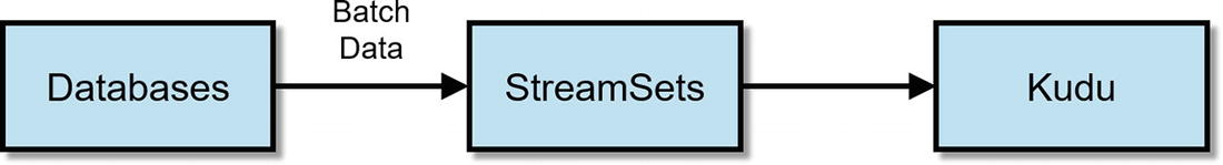
Batch data ingestion with StreamSets and Kudu
Internet of Things (IoT)
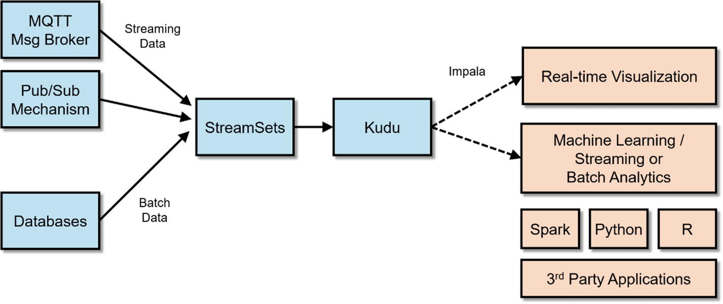
StreamSets IoT Architecture
Deployment Options
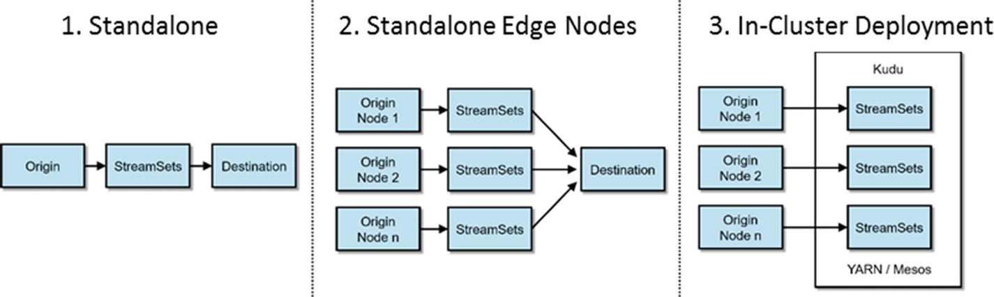
StreamSets Deployment Options
Consult the Data Collector User Guide for information on installing StreamSets from a Tar ball (Service Start), an RPM Package (Service Start), and Cloudera Manager (Cluster Mode).
Using StreamSets Data Collector
Let’s start by creating our first pipeline. Navigate to the StreamSets Data Collector URL, and you will be presented with a login page. The default username is “admin.” The default password is “admin.” Log in, then click “Create New Pipeline.” When prompted, enter a title and description for your new pipeline (see Figure 7-6).
StreamSets Console
Ingesting XML to Kudu
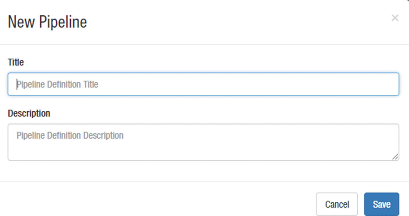
New Pipeline
Directory Origin
XML Parser
Kudu destination
Before we can start configuring our stages, we need to create the directory that will serve as the origin of our data source and the destination Kudu table. We’ll also prepare some test data.
Open impala-shell and create a table.
Log in to the Cloudera cluster and create a directory that will contain our sensor data.
Let’s create some test data that we will use later in the exercise.
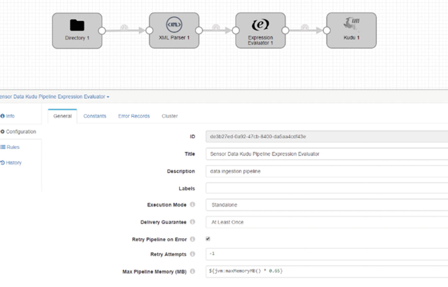
Configure Pipeline
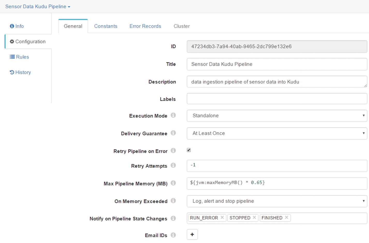
Configure Pipeline
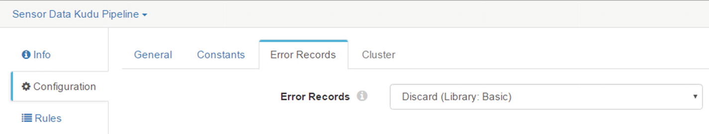
Error Records
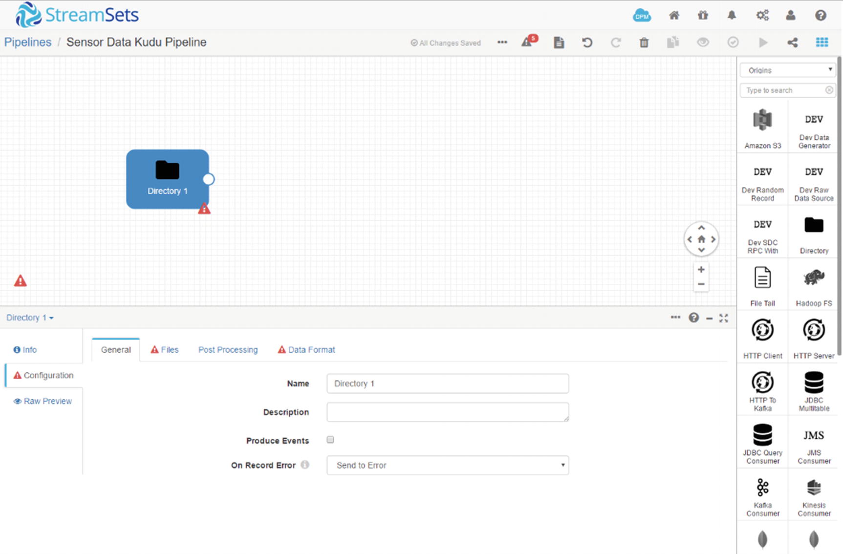
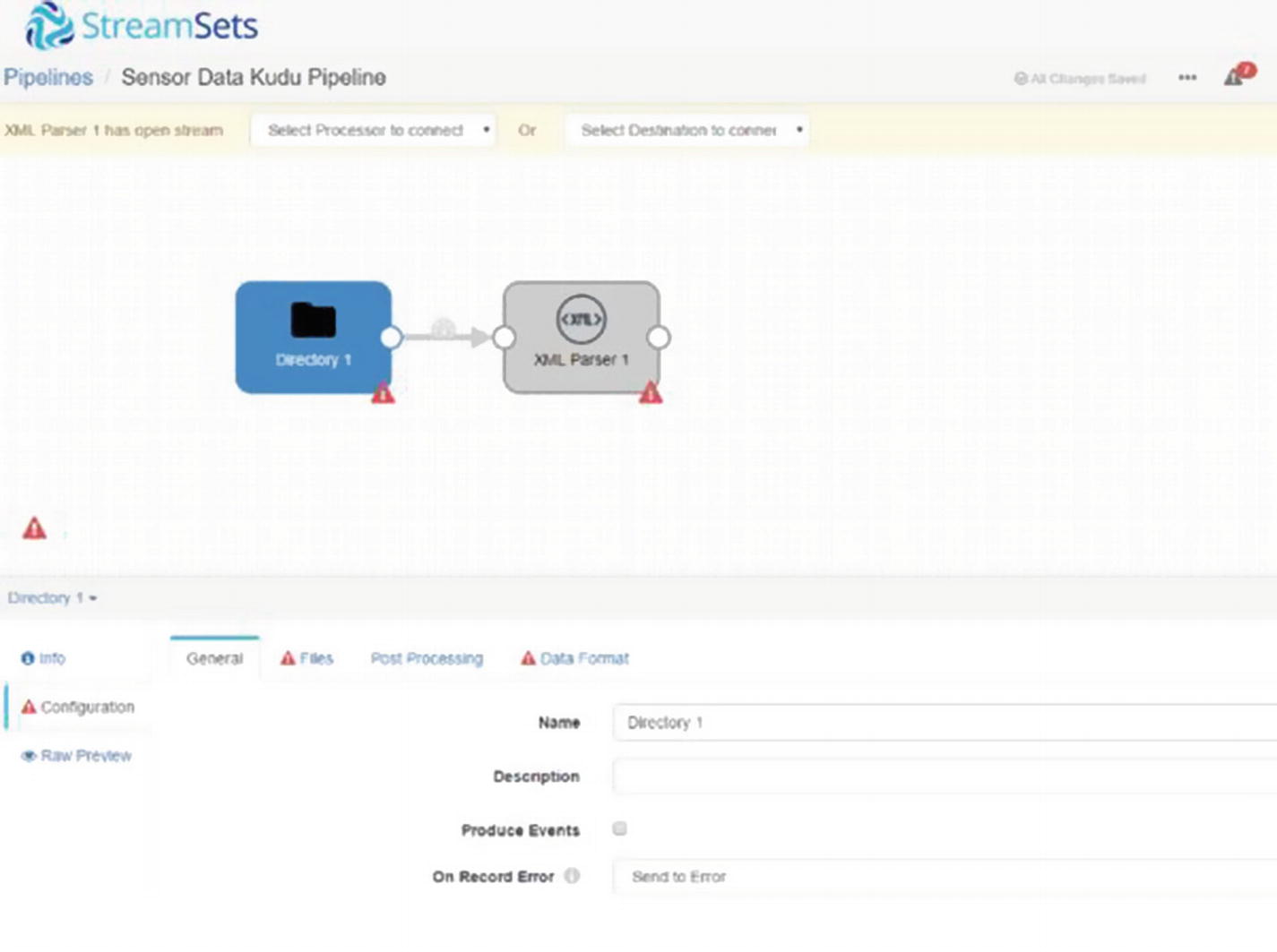
Configure the Directory Origin
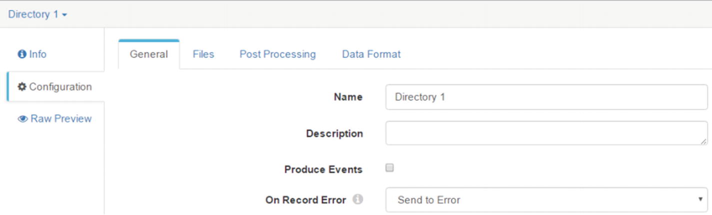
Configure Directory origin
The “General” allows users to specify a name and description for the origin. There’s an option to enable the origin to generate events. If you enable “Produce Events,” the directory origin produces event records every time the directory origin begins or ends reading a file. You can ignore this configuration item for now. “On Record Error” allows you to choose an action to take on records sent to error. The default option is “Send to Error.” The other options are “Discard” and “Stop Pipeline.” Leave the default option for now.
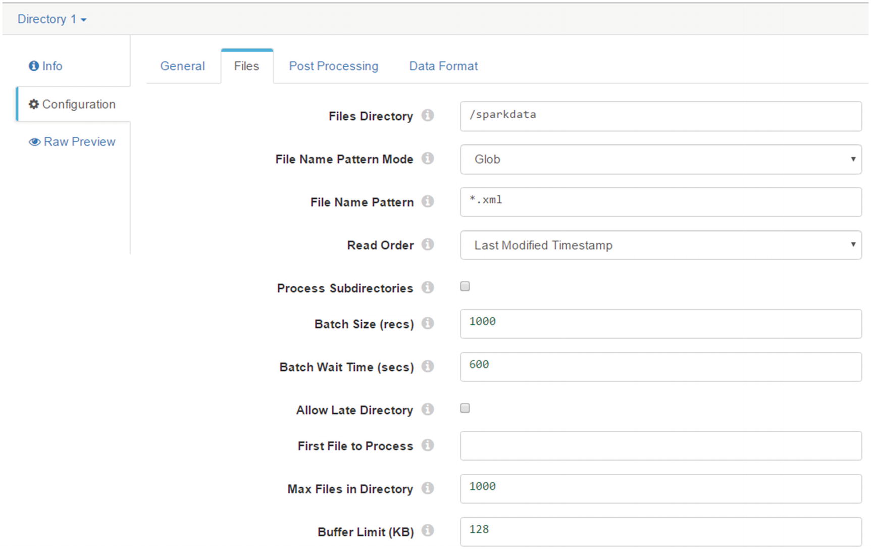
The “Files” tab contains various configuration options related to file ingestion. The most interesting option for us in our examples are “Files Directory,” which is the local directory where you want to place files you want to ingest. “File Name Pattern Mode” lets you select whether the file name pattern specified uses regex syntax or glob syntax. Leave it set to “Glob” for now. “File Name Pattern” is an expression that defines the pattern of the file names in the directory. Since we’re ingesting XML files, let’s set the pattern to “*.xml”. “Read Order” controls the order of how files are read and processed by Data Collector. There are two options, “Last Modified Timestamp” and “Lexicographically Ascending File Names.” When lexicographically ascending file names are used, files are read in lexicographically ascending order based on file names. x It’s important to note that this ordering will order numbers 1, 2, 3, 4, 5, 6, 7, 8, 9, 10, 11, 12, 13, 14, 15 as 1, 10, 11, 12, 13, 14, 15, 2, 3, 4, 5, 6, 7, 8, 9.If you must read files in lexicographically ascending order, consider adding leading zeros to the file names such as: file_001.xml, file_002.xml, file_003.xml, file_004.xml, file_010.xml, file_011.xml, file_012.xml.
Last Modified Timestamp
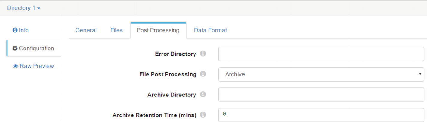
Archive
Data Format
Configure the XML Parser Processor
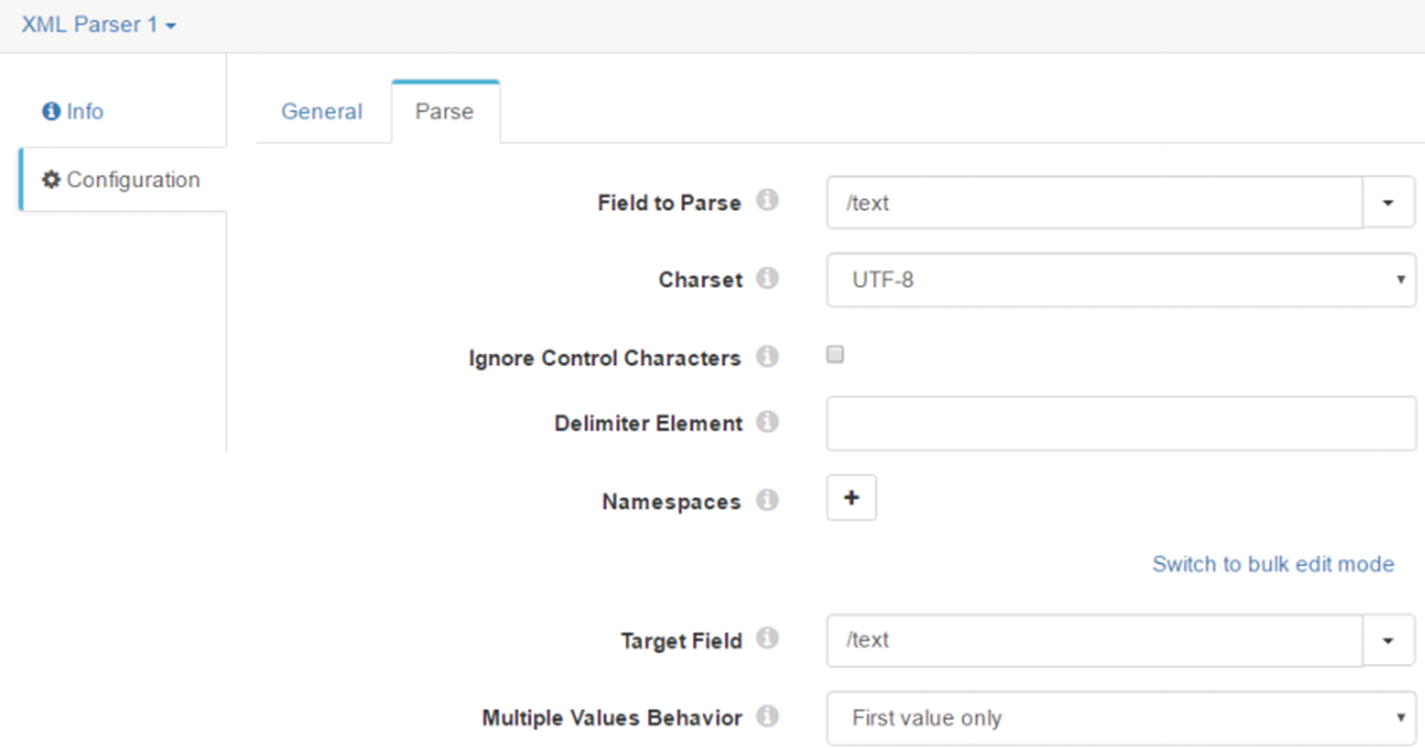
Parse tab
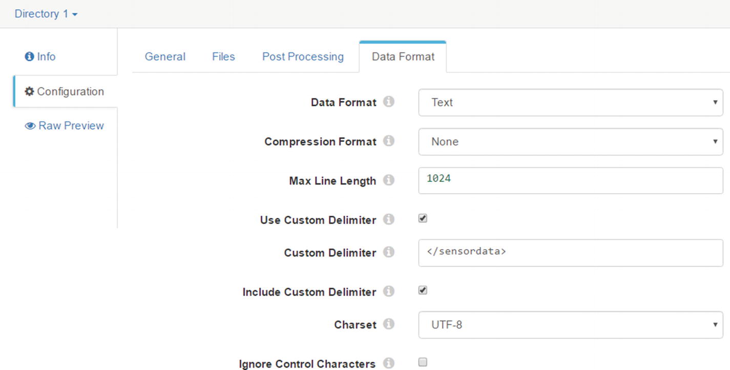
When the Directory origins processes our XML data, it will create two records, delimited by “</sensordata>.”
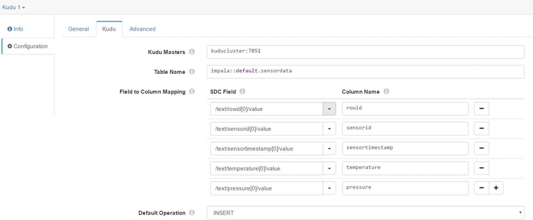
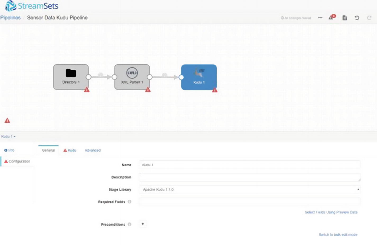
Kudu tab
Validate and Preview Pipeline
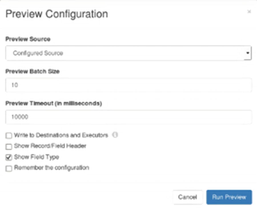
Preview Configuration
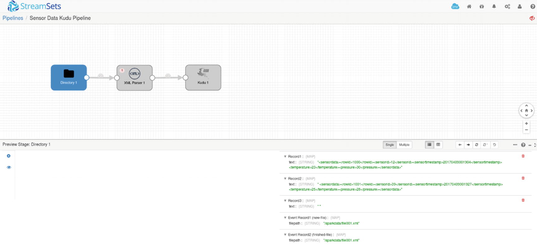
Preview – inspecting records
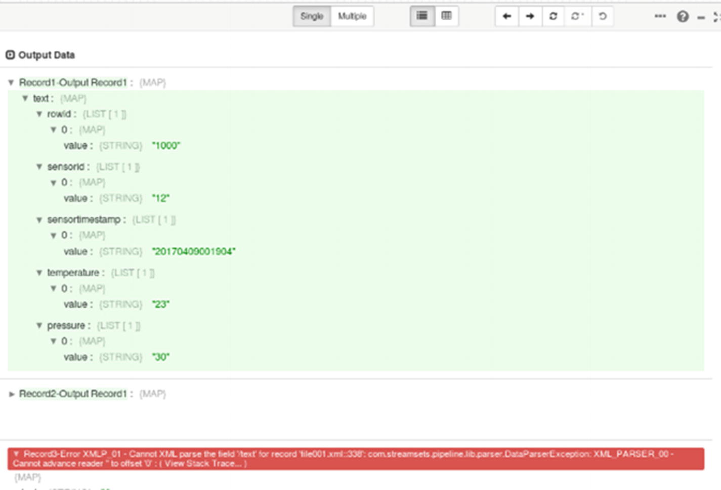
Preview – error processing empty record
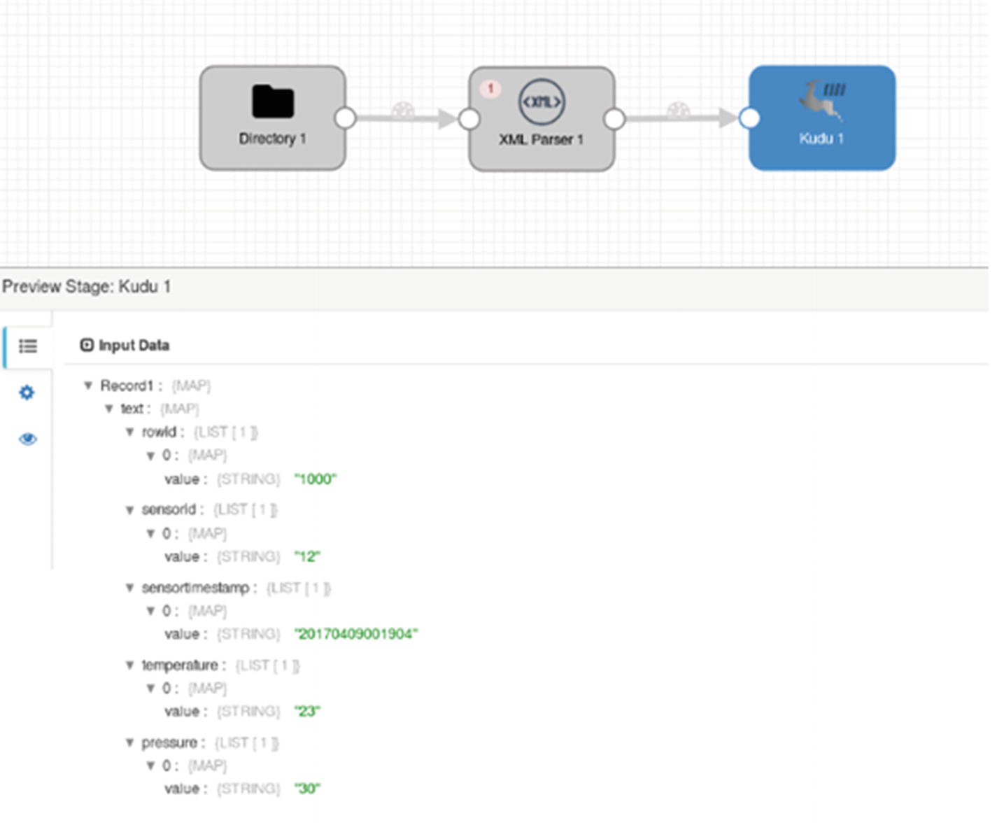
Preview – Kudu destination
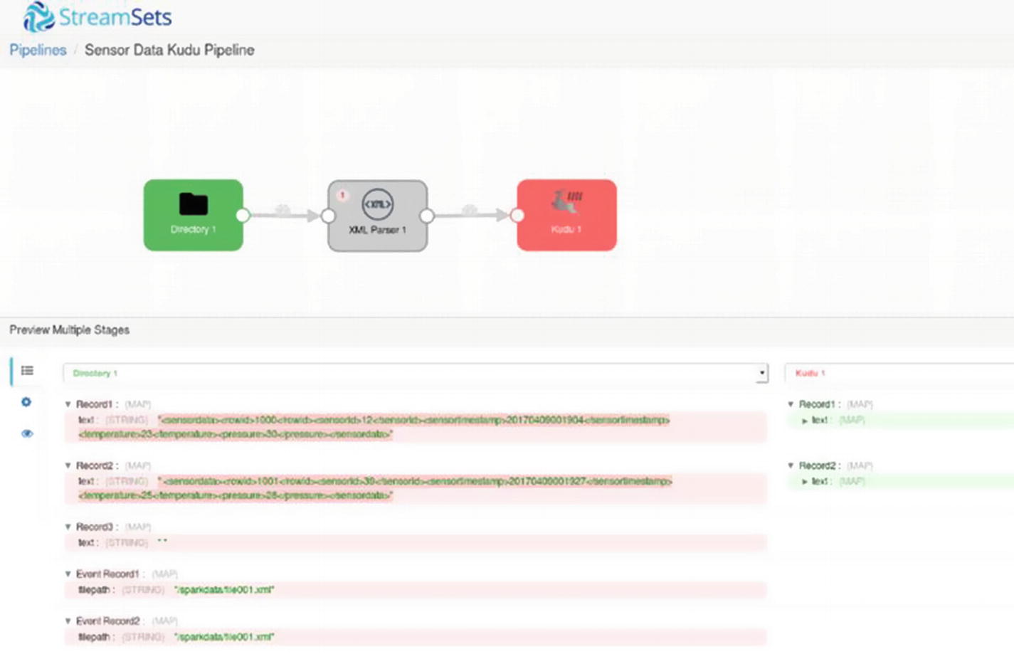
Preview – Multiple Stages
Start the Pipeline
Now you’re ready to start the pipeline. Click the start icon, and then copy our test data (file001.xml) to /sparkdata.
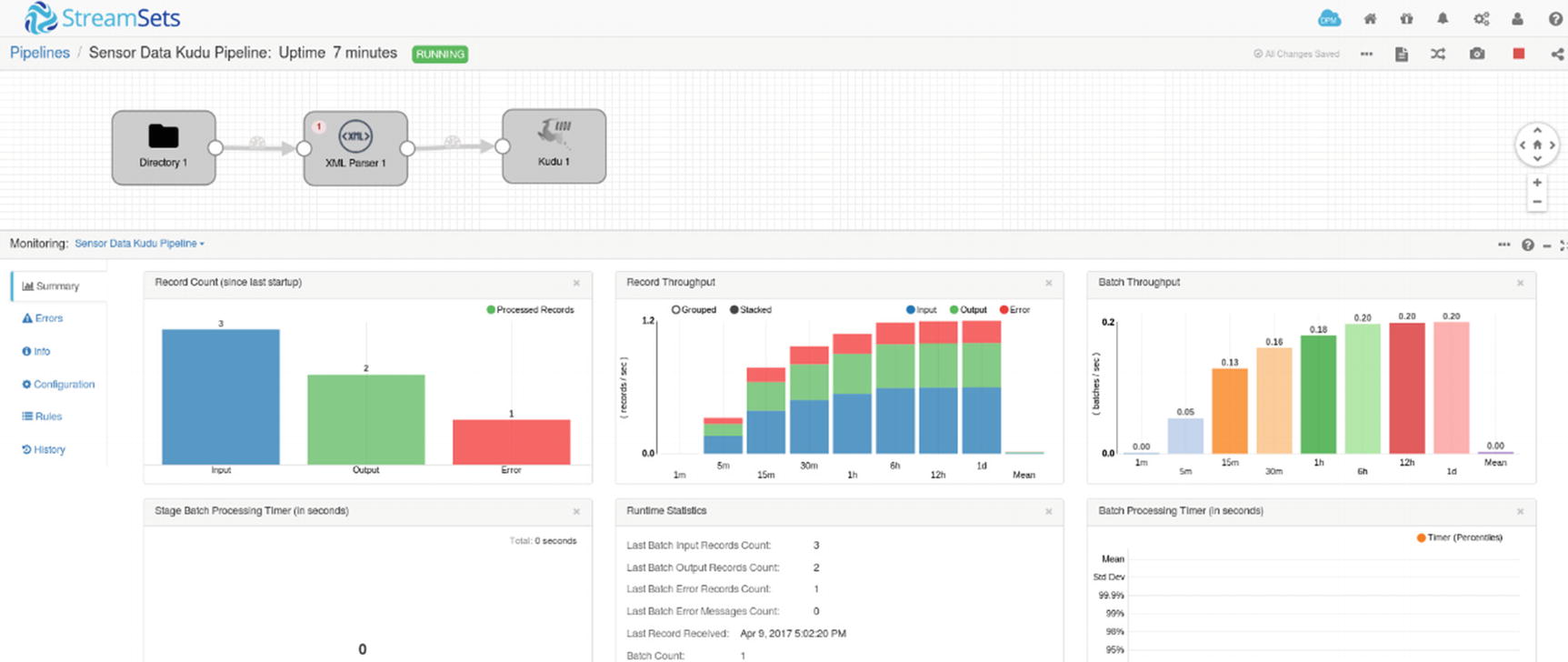
Monitoring pipeline
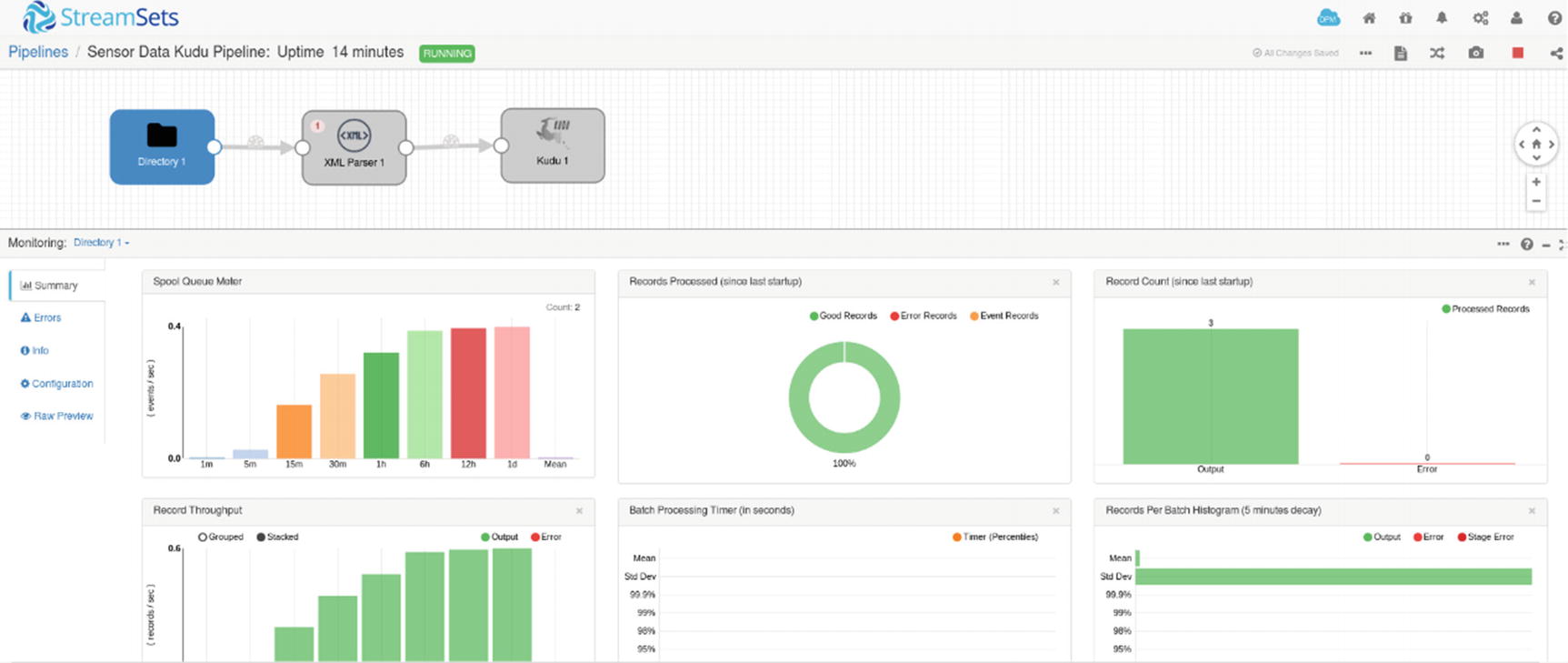
Monitoring– Directory Origin
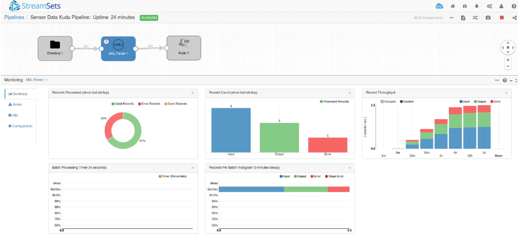
Monitoring – XML Parser
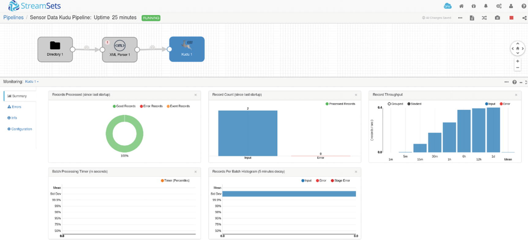
Monitoring – Kudu destination
Let’s verify if the rows were indeed successfully inserted in Kudu. Start impala-shell and query the sensordata table.
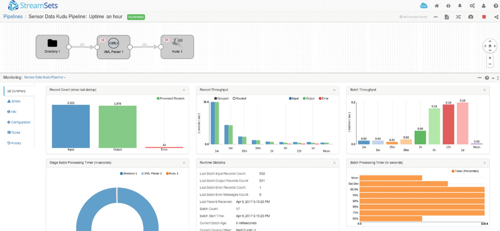
Monitoring pipeline after one hour
Congratulations! You’ve successfully built and run your first StreamSets data pipeline.
Stream Selector
There are times when you have a requirement to route data to certain streams based on conditions. For example, you can insert data to certain tables based on “Country.” There is a default stream that handles records that do not match any of the user-defined conditions. xiv
In this pipeline, all records where “Country” matches USA goes to Stream 1, Canada goes to Stream 2, and Brazil goes to Stream 3. Everything else goes to Stream 4. You’ll be able to specify these conditions using the Stream Selector.
Let’s design another pipeline. Instead of starting from scratch, let’s make a copy of the pipeline we just created and modify it to use a Stream Selector. In this example, we’ll write to three different versions of the XML data to three different Kudu tables. Here’s what our new XML data looks like. The Stream Selector will examine the value of firmwareversion.
We’ll create two more Kudu tables: sensordata2 and sensordata3. We’ll also add a firmwareversion column in the existing sensordata table. We’ll have a total of three sensordata tables, each with a different set of columns.
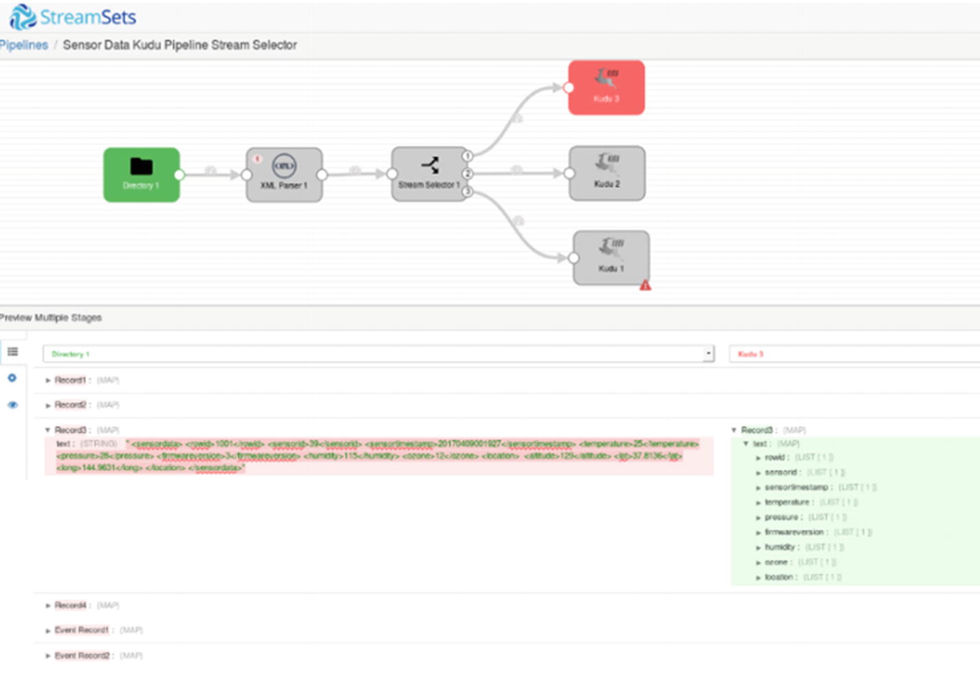
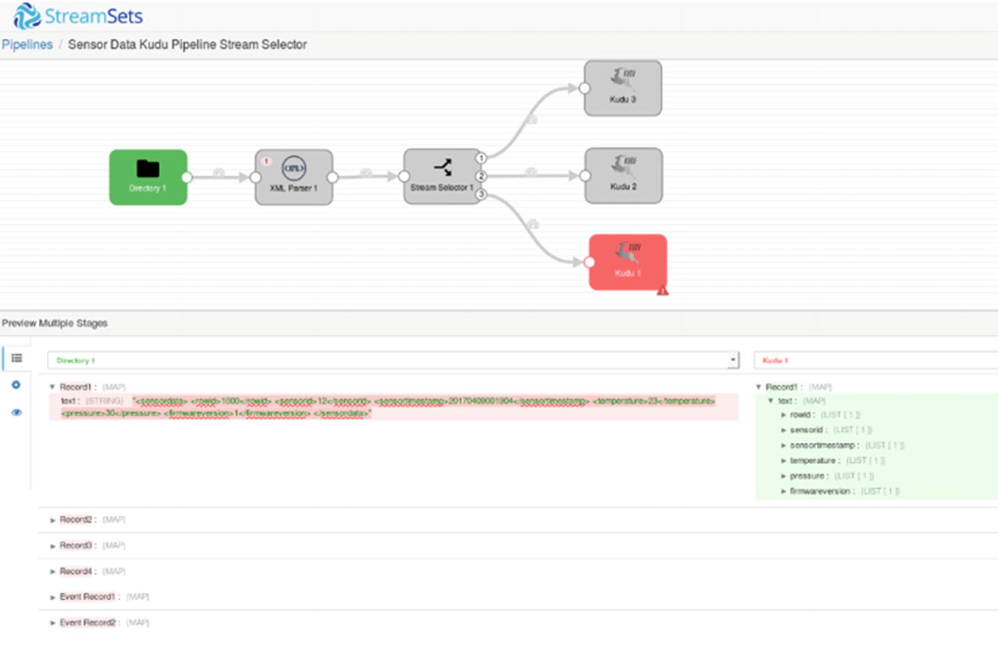
Drag a Stream Selector processor and two more Kudu destinations onto the canvas. Connect the XML Parser to the Stream Connector. You need to define three conditions: XML data with firmwareversion of 1 (or any value other than 2 or 3) goes to default stream (Kudu 1), XML data with firmwareversion 2 goes to stream 2 (Kudu 2), and finally XML data with firmwareversion 3 goes to stream 3 (Kudu 3).
Add two more conditions to the Stream Selector processor with these conditions.
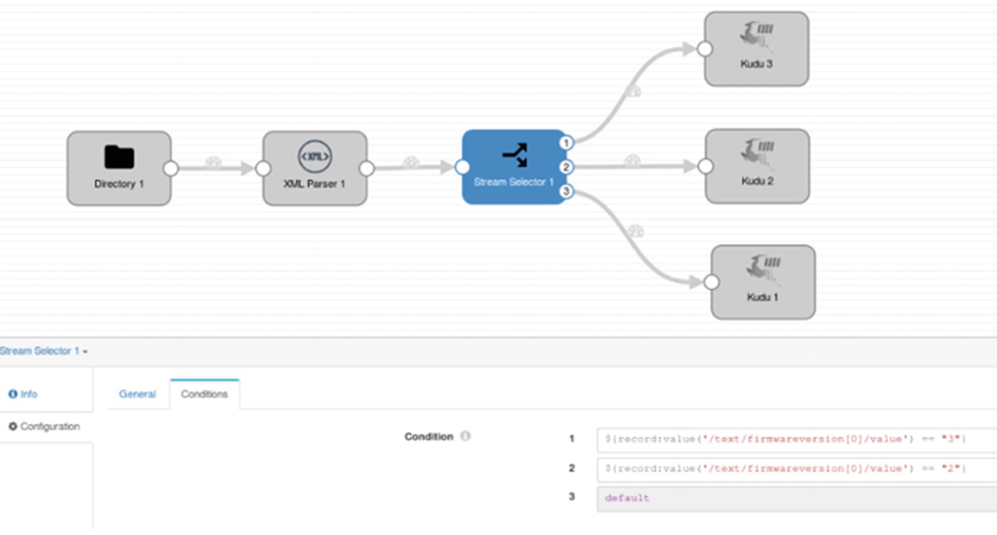
Stream Selector
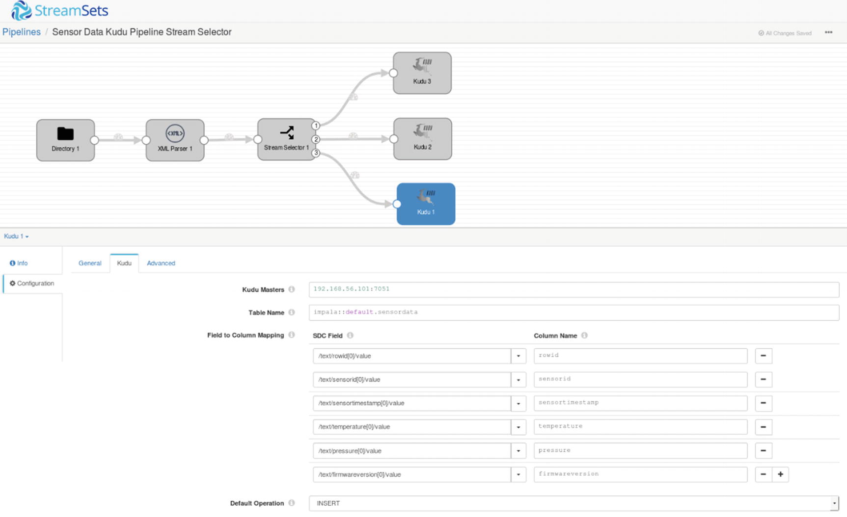
First Kudu destination
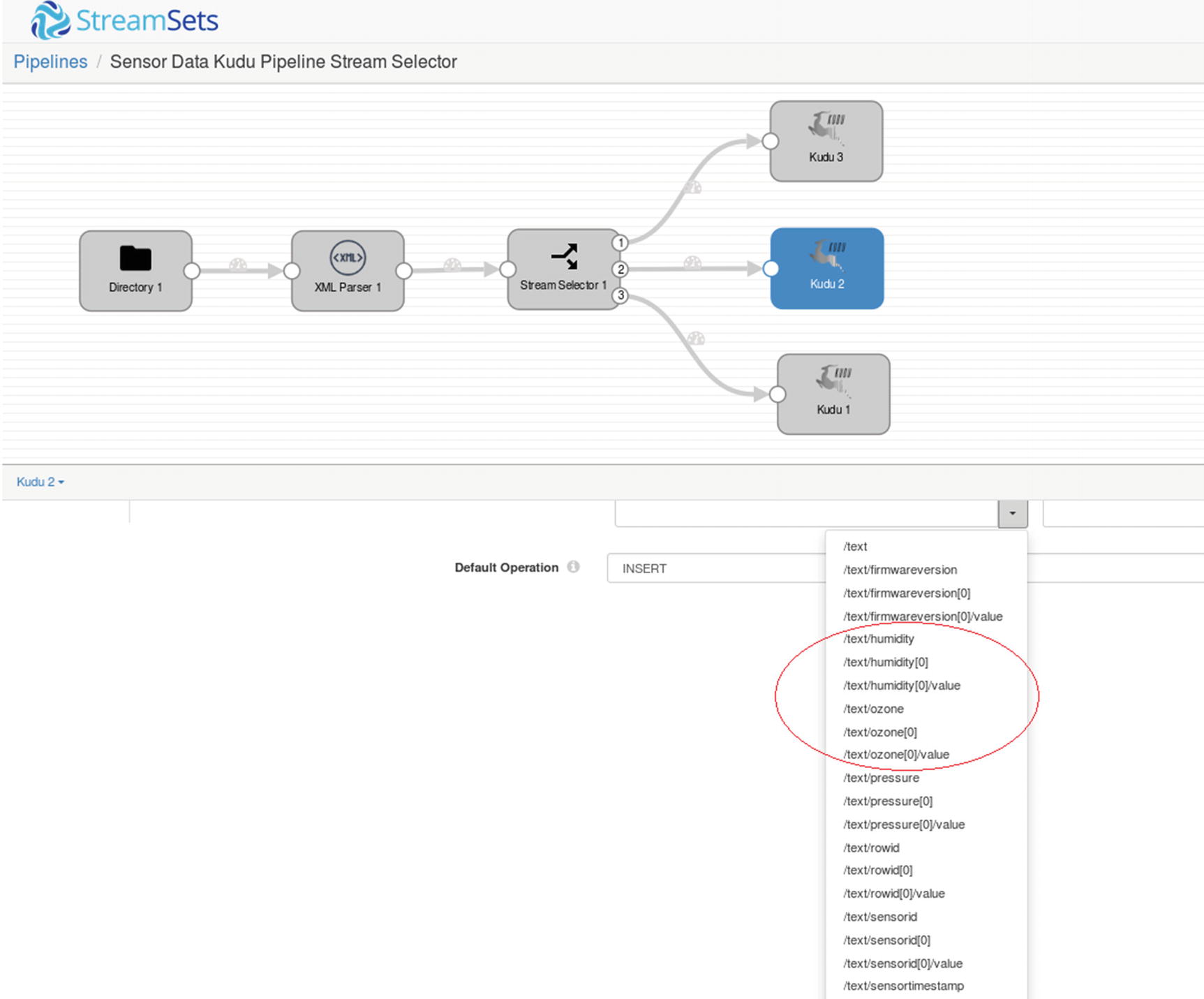
Second Kudu destination
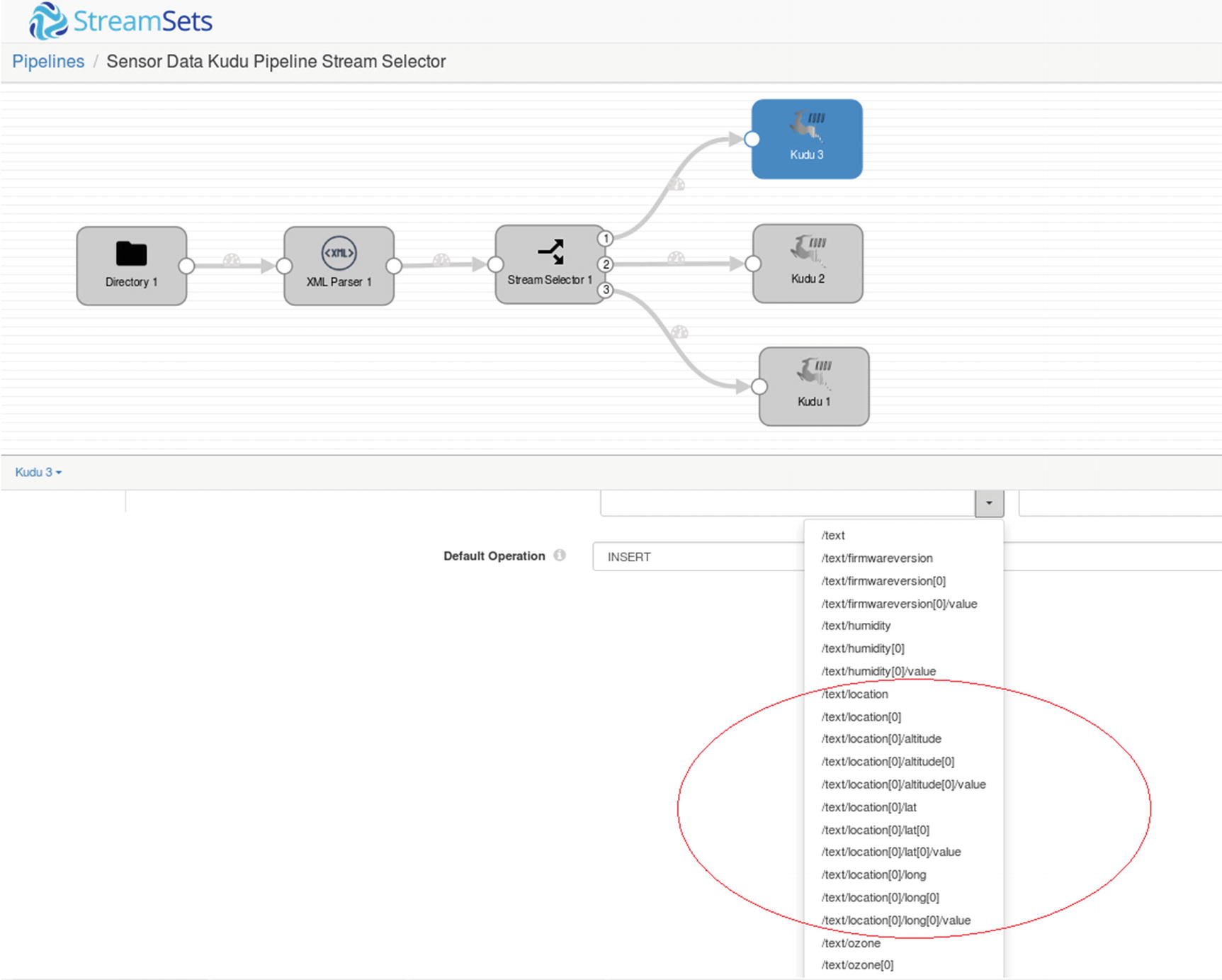
Third Kudu destination
Preview – First Kudu destination
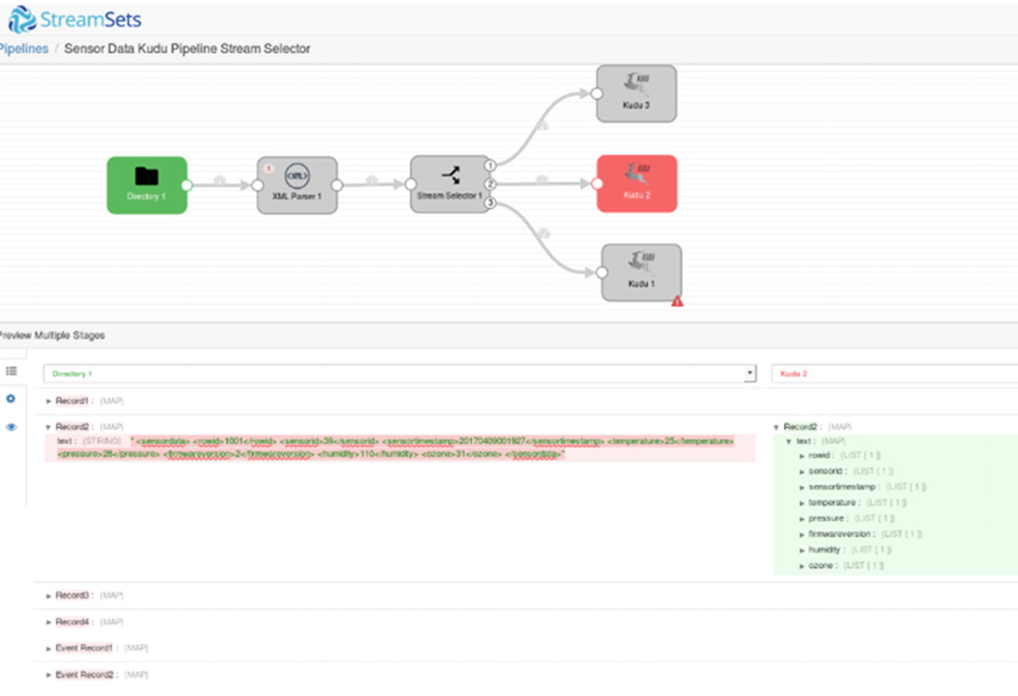
Preview – Second Kudu destination
Preview – Third Kudu destination
Before you start the pipeline, confirm that the destination Kudu tables are empty from the impala-shell.
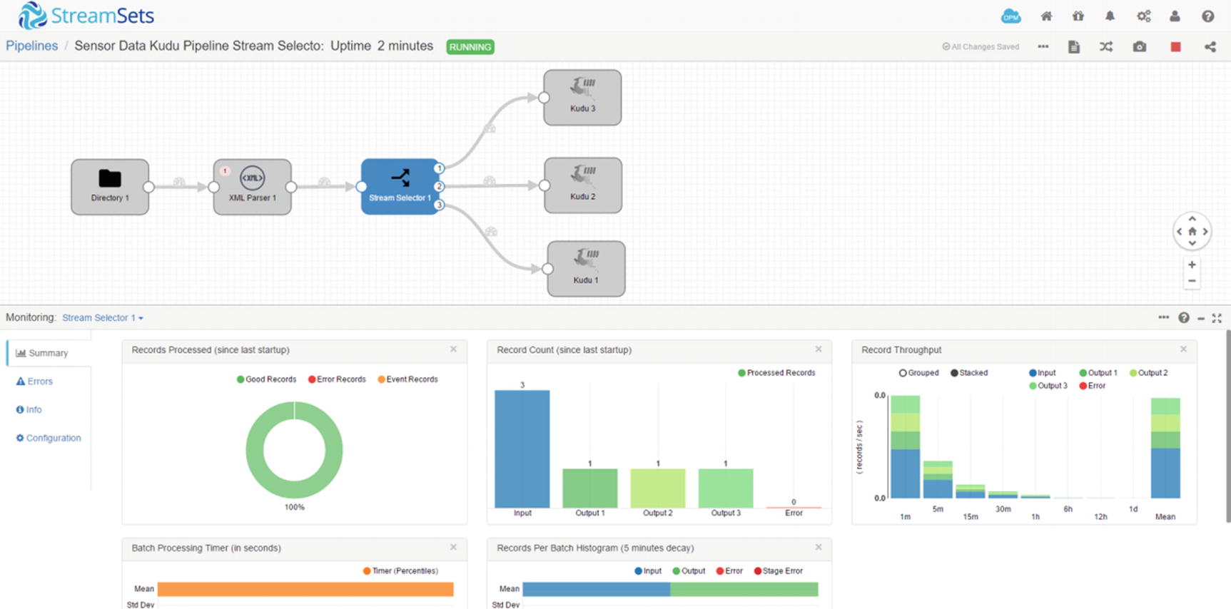
Monitor Stream Selector (Figure 7-36)
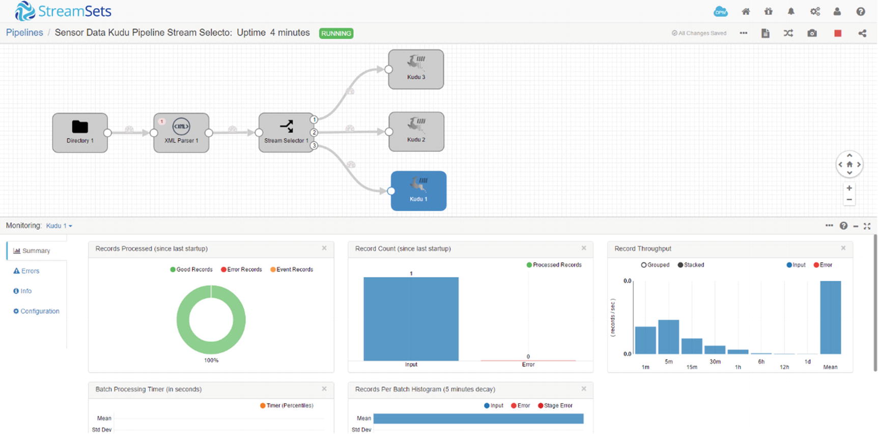
Monitor Kudu destination (Figure 7-37)
Check the Kudu tables to confirm that the records were successfully ingested.
Expression Evaluator
The Expression Evaluator allows users to perform data transformations and calculations and writes the results to new or existing fields. Users can also add or change field attributes and record header attributes. xv I often use the Expression Evaluator as a rules engine.
Let’s work on a new example. We’ll use an Expression Evaluator to perform two data transformations. We’ll convert the temperature from Celsius to Fahrenheit and save it to the existing temperature field. For the second transformation, we’ll update a new status field with the values “NORMAL,” “WARNING,” or “CRITICAL” depending on the values of the pressure field. If pressure is over 40, the status field gets updated with “WARNING,” and if pressure is over 50 it gets updated with “CRITICAL.” Let’s get started.
Add another “status” column to the Kudu sensordata table.
We’ll use the following XML data for this example.
Expression Evaluator
Click the Expression Evaluator processor (Figure 7-38) and navigate to the “Expressions” tab. We’ll add two entries in the “Field Expressions” section. For the first entry, in the “Output Field” enter the following value:
In the “Field Expression”, enter the expression:
This is the formula to convert temperature from Celsius to Fahrenheit. Specifying an existing field in the “Output Field” will overwrite the value in the field.
For the second entry, we’ll use an if-then-else expression. Enter a new field in the “Output Field”:
Enter the expression in “Field Expression”:
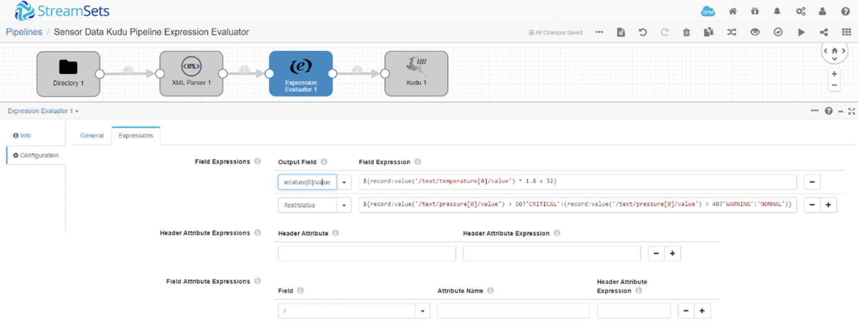
Expression Evaluator - Expression
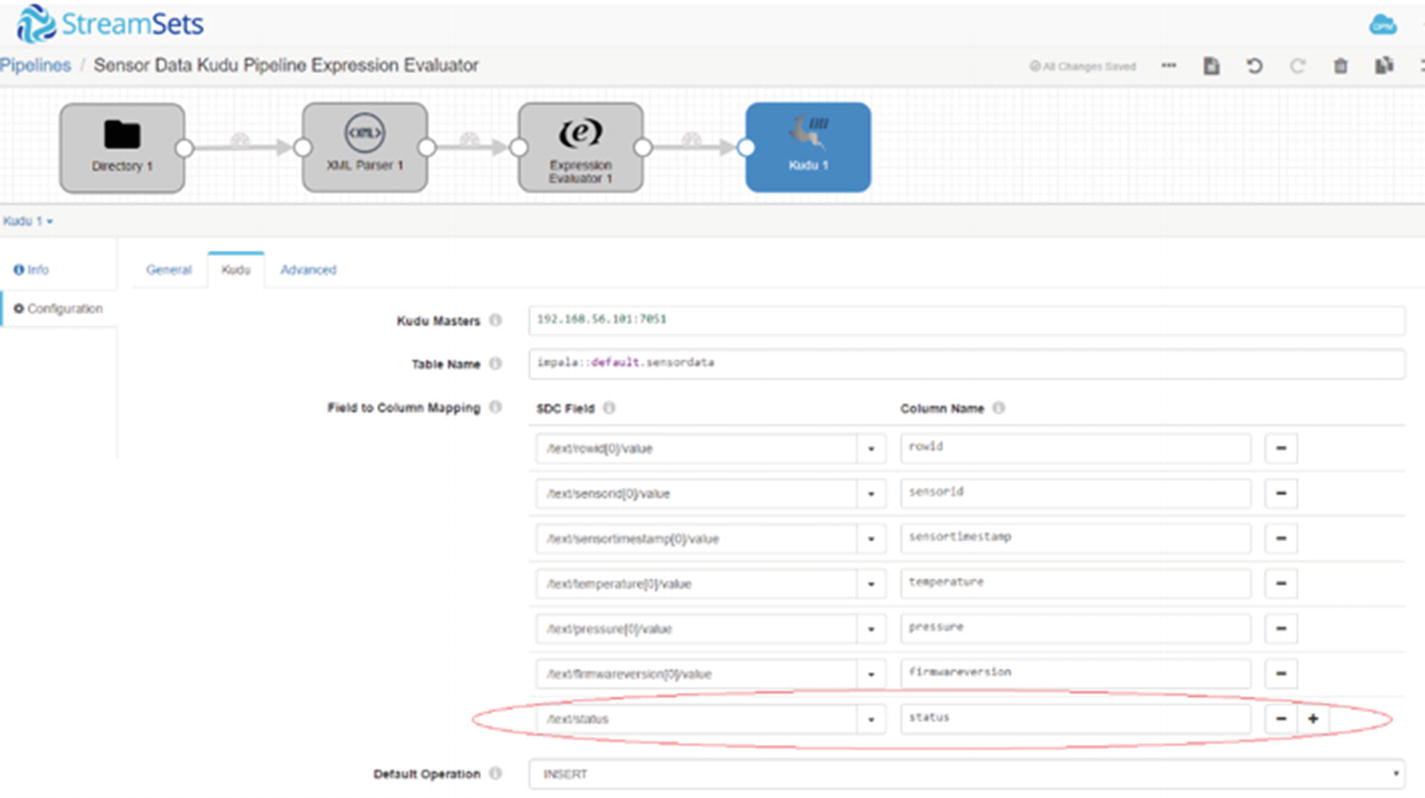
Map SDC field to Kudu field
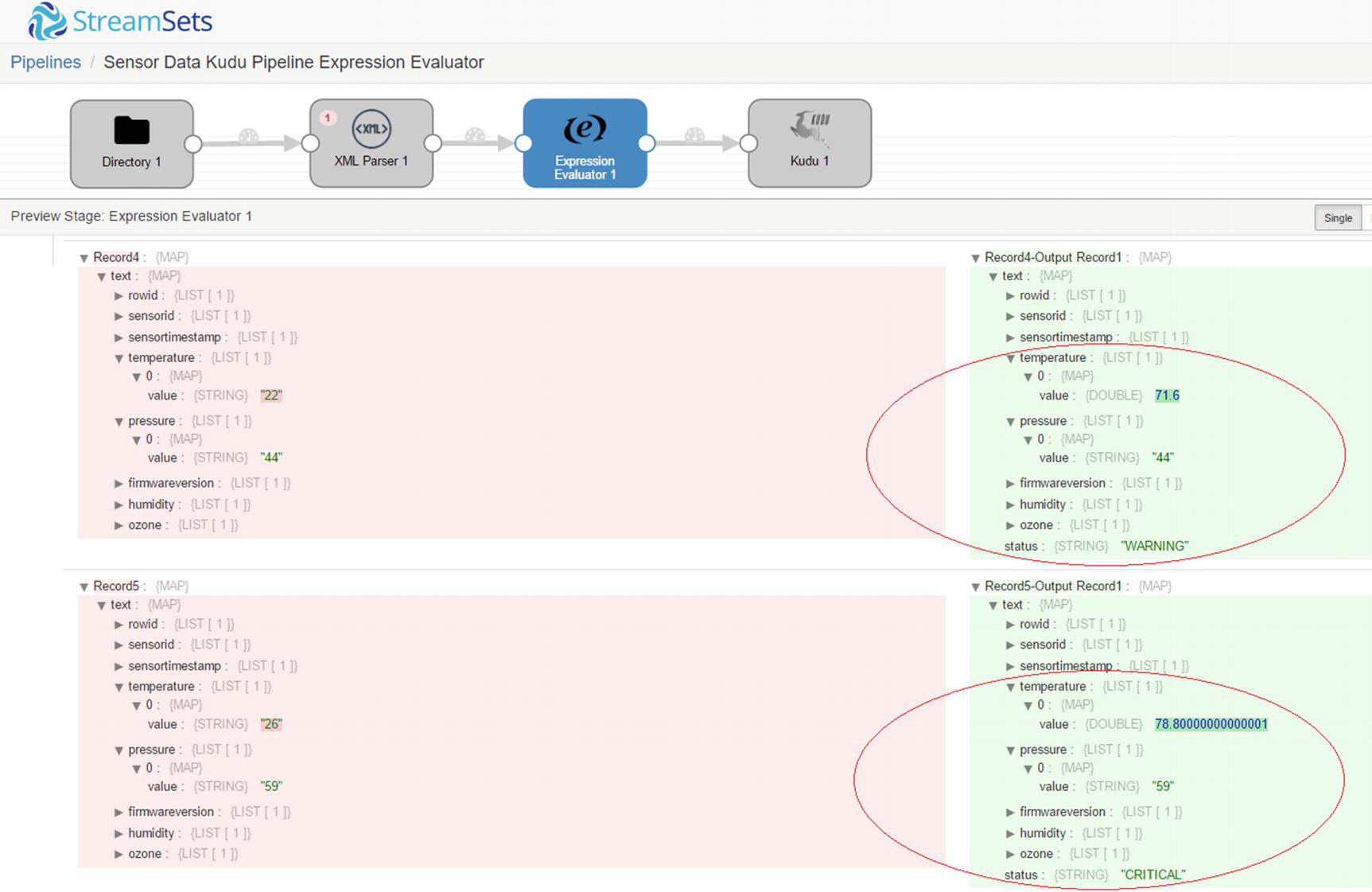
Preview – Expression Evaluator
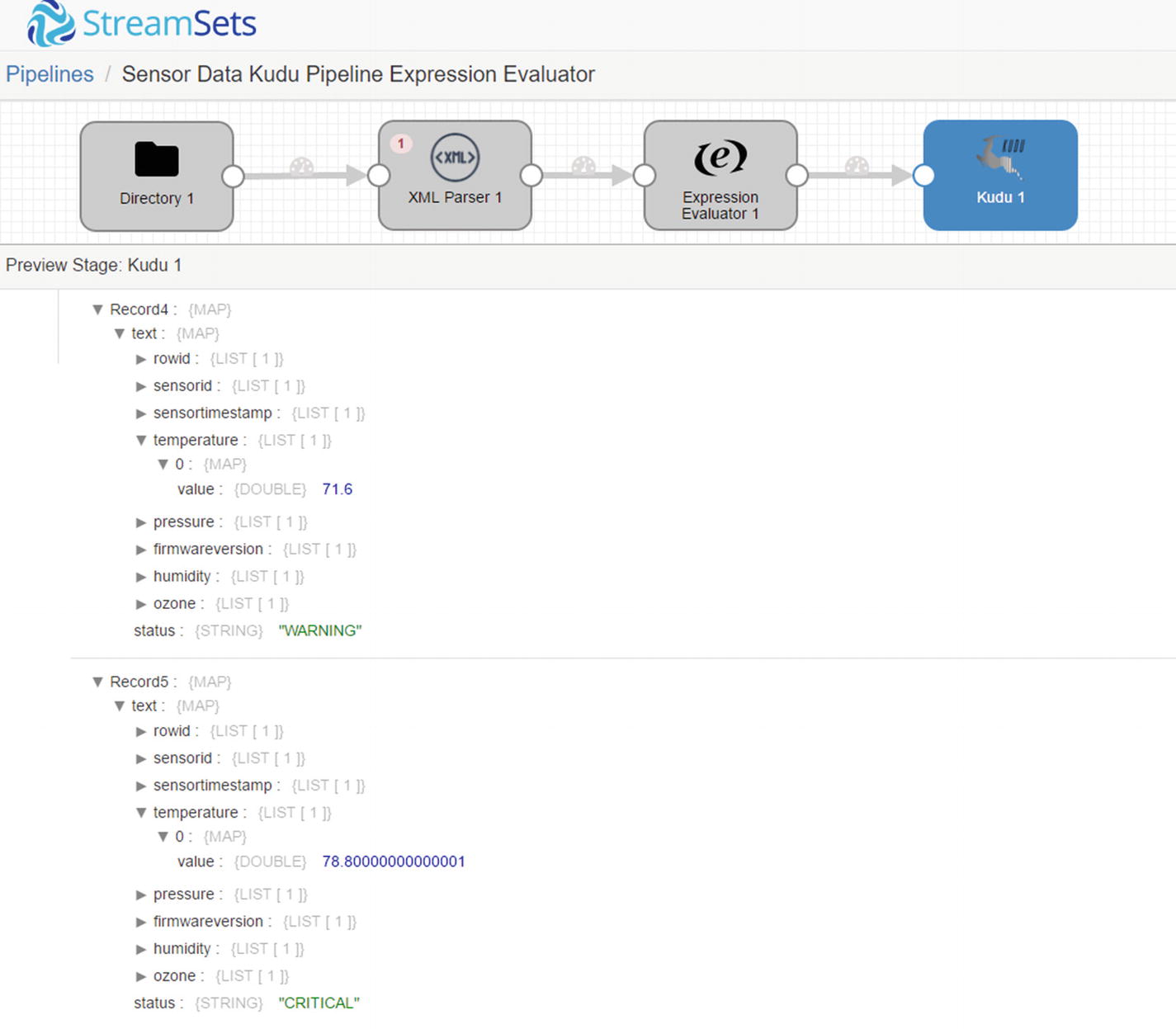
Preview – Kudu destination
Run the pipeline and copy the XML file to /sparkdata.
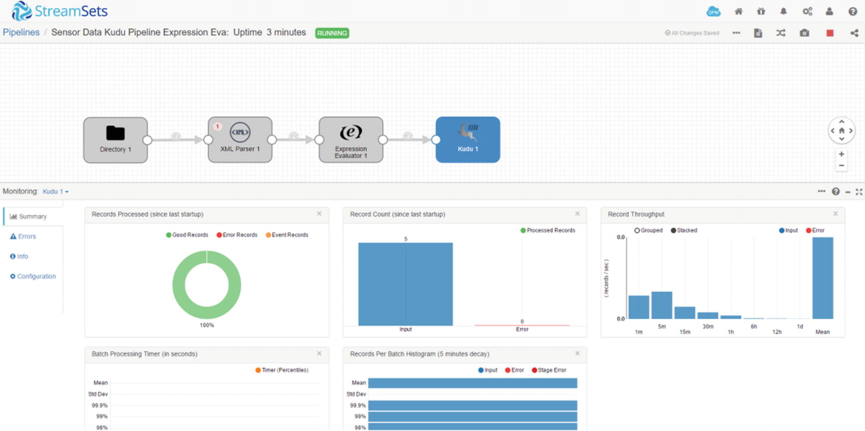
Five records inserted into Kudu destination
Confirm that the data were successfully inserted to Kudu. As you can see the status field was successfully updated based on pressure. Also, the temperatures are now in Fahrenheit.
Using the JavaScript Evaluator
StreamSets Data Collector includes a JavaScript evaluator that you can use for more complex processing and transformation. It uses JavaScript code to process one record or one batch at a time. xvi As you can imagine, processing one record at a time will most likely be slower compared to processing by batch of data at a time. Processing by batch is recommended in production environments.
Although we’re using JavaScript in this example, other languages are supported by Data Collector. In addition to JavaScript, you can use Java, Jython (Python), Groovy, and Spark Evaluators. These evaluators enable users to perform more advanced complex stream processing, taking advantage of the full capabilities of each programming languages.
Let’s start with a simple example. We’ll create two additional fields, action and uniqueid. We’ll generate the value of action based on the value of the status field. Next, we’ll generate a universally unique identifier (UUID) using a custom JavaScript function. We’ll save this UUID in our uniqueid field.
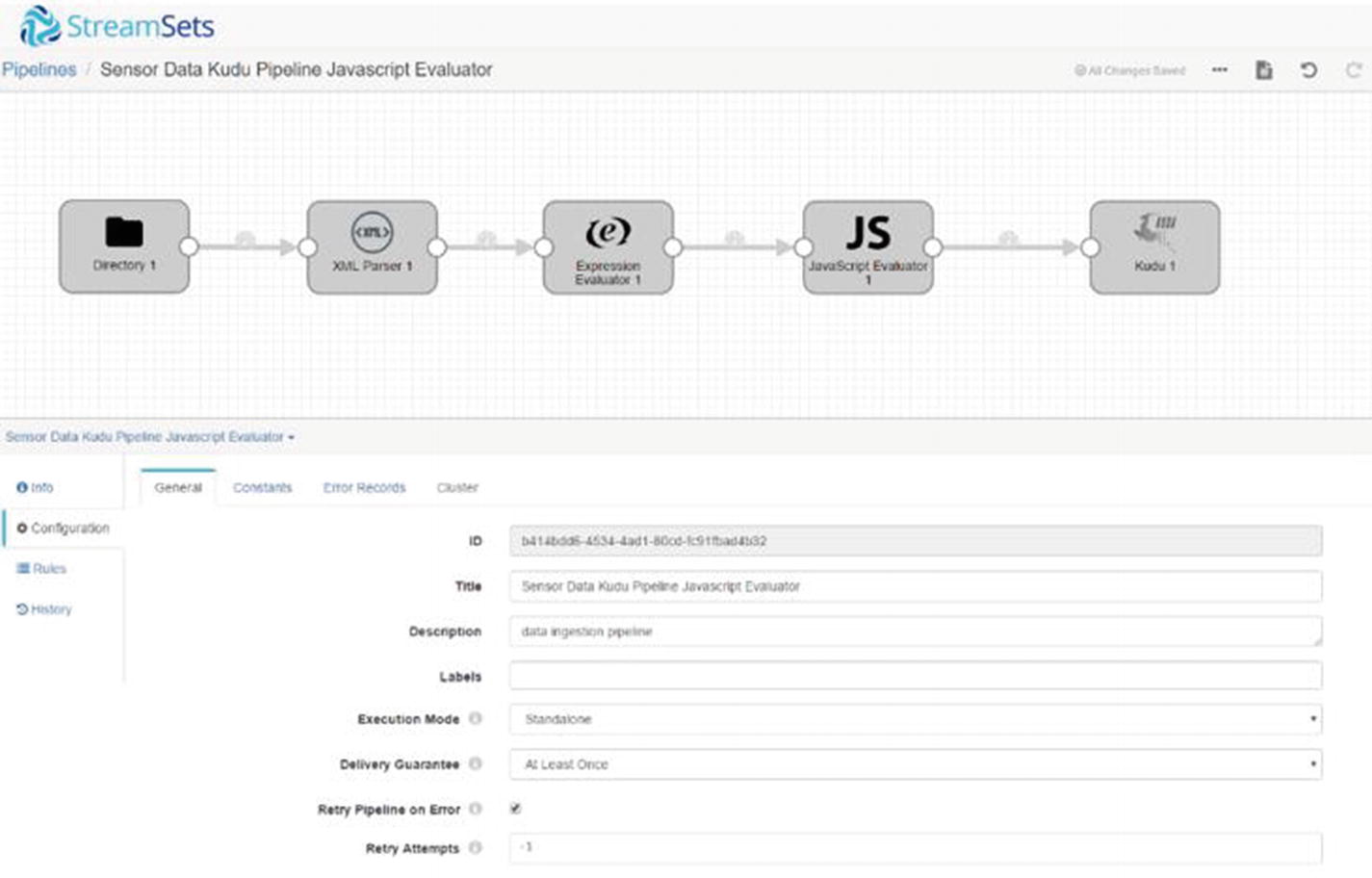
JavaScript Evaluator
Now let’s configure the JavaScript Evaluator to use our custom JavaScript code in our pipeline. In the Properties panel, on the JavaScript tab, make sure that “Record Processing Mode” is set to “Batch by Batch.” “Script” will contain your customer JavaScript code. As mentioned earlier, we’ll create a function to generate a UUID. xvii The JavaScript Evaluator passes the batch to the script as an array. To access individual fields, use the format: records[arrayindex].value.text.columname. To refer to the value of the status field use “records[i].value.text.status.” We also created a new field, “record[i].value.text.action” using this format. See Listing 7-1.
Javascript Evaluator code

JavaScript Evaluator code
Add the action and uniqueid columns to the Kudu sensordata columns.
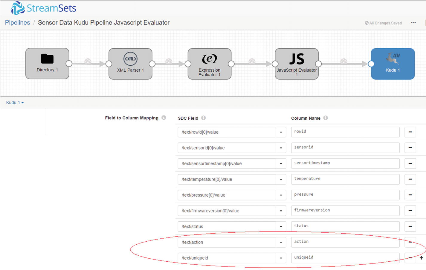
Map SDC field
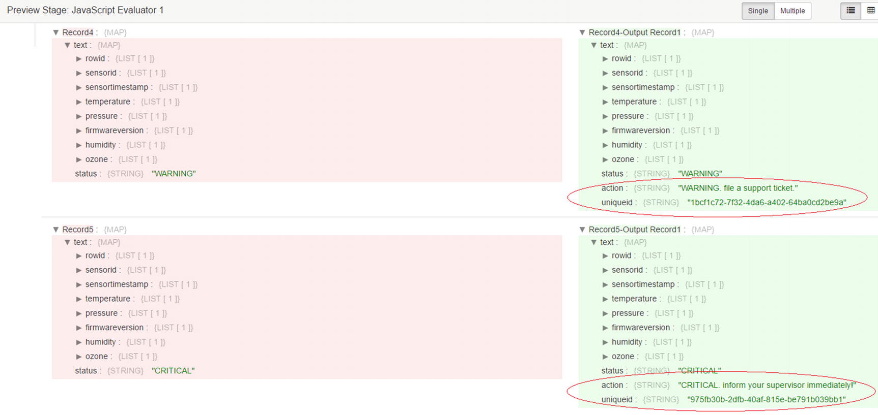
Preview values
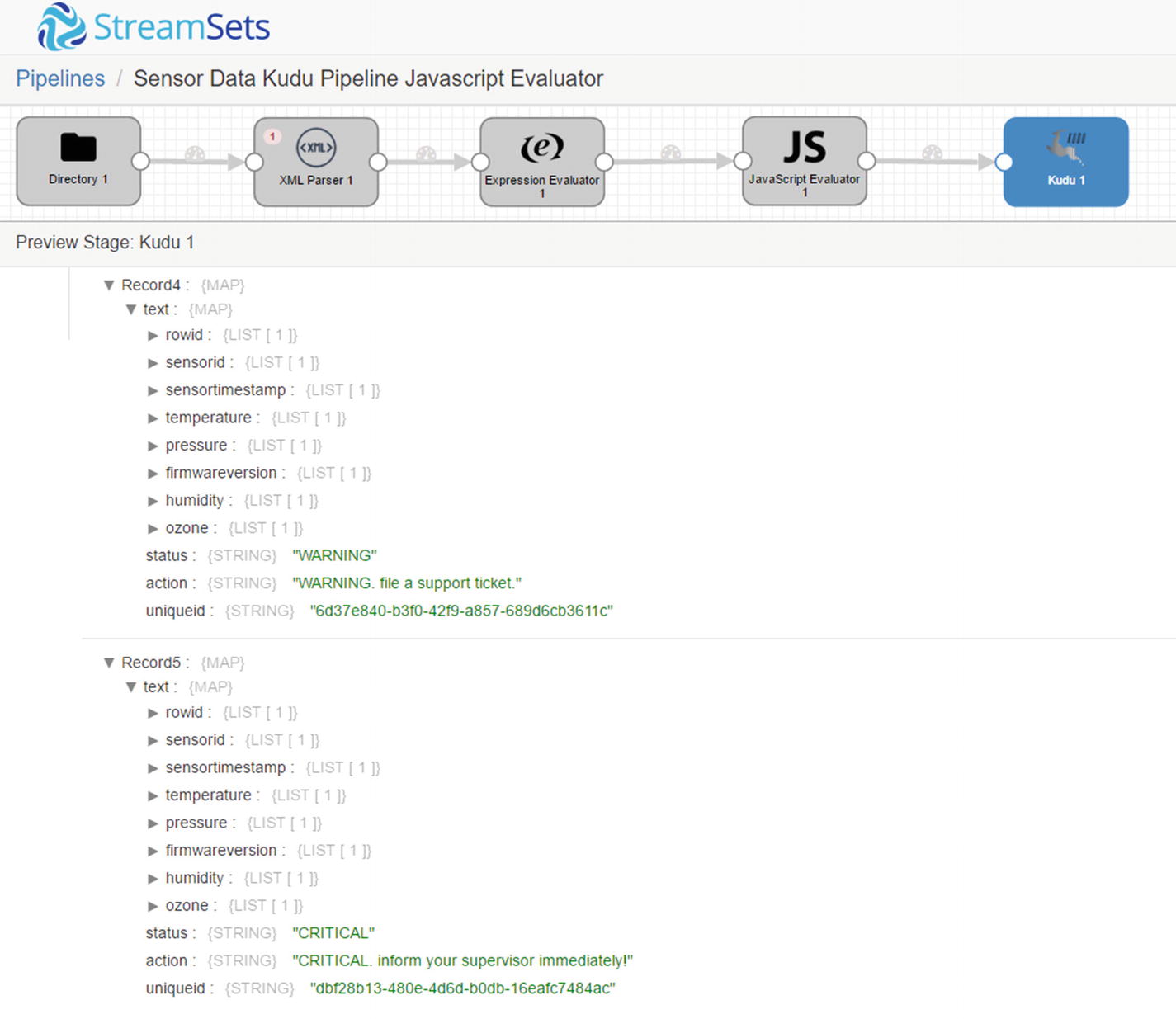
Confirm values in Kudu destination
Run the pipeline and copy the XML file to /sparkdata.
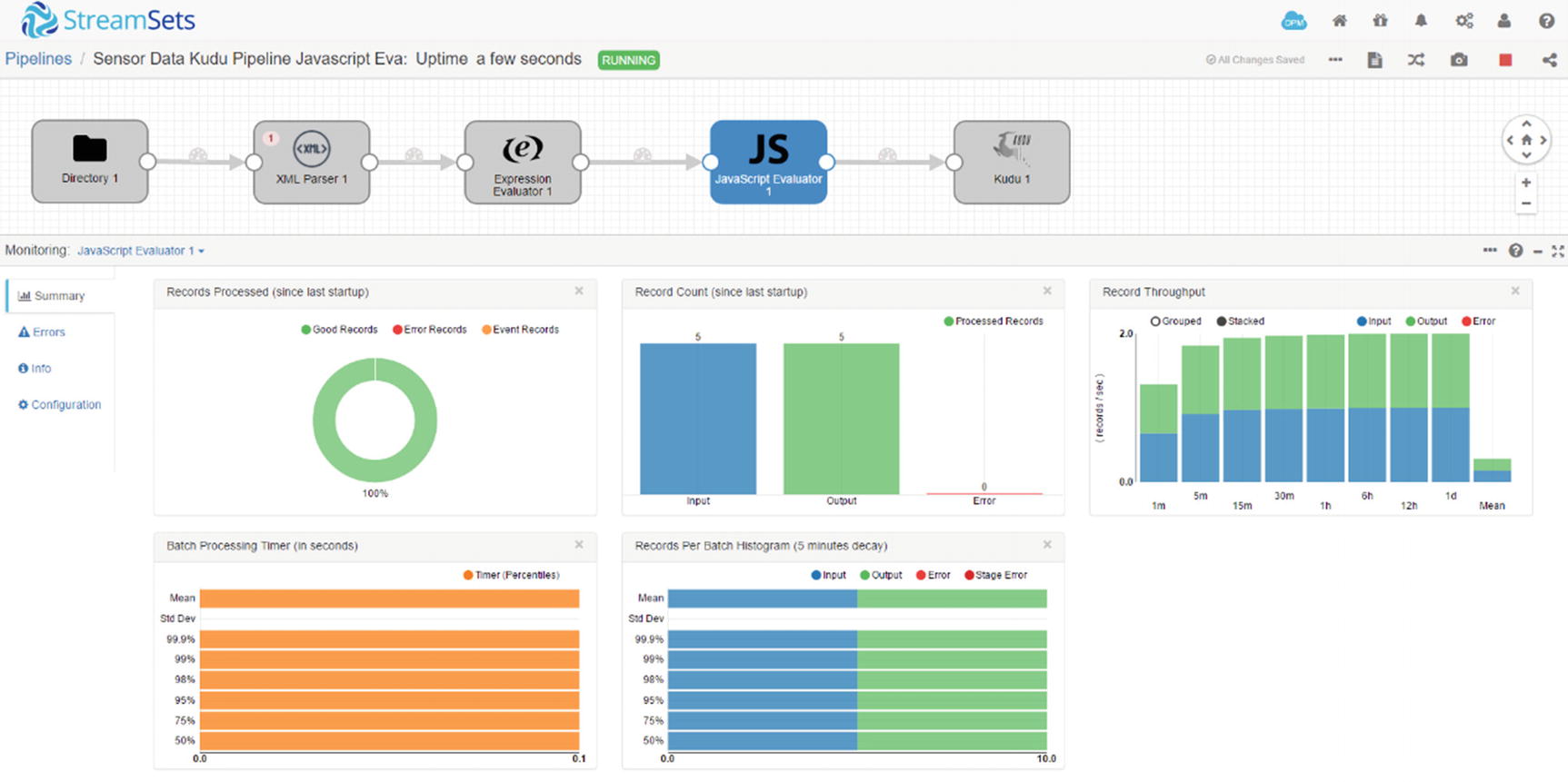
Monitor JavaScript Evaluator
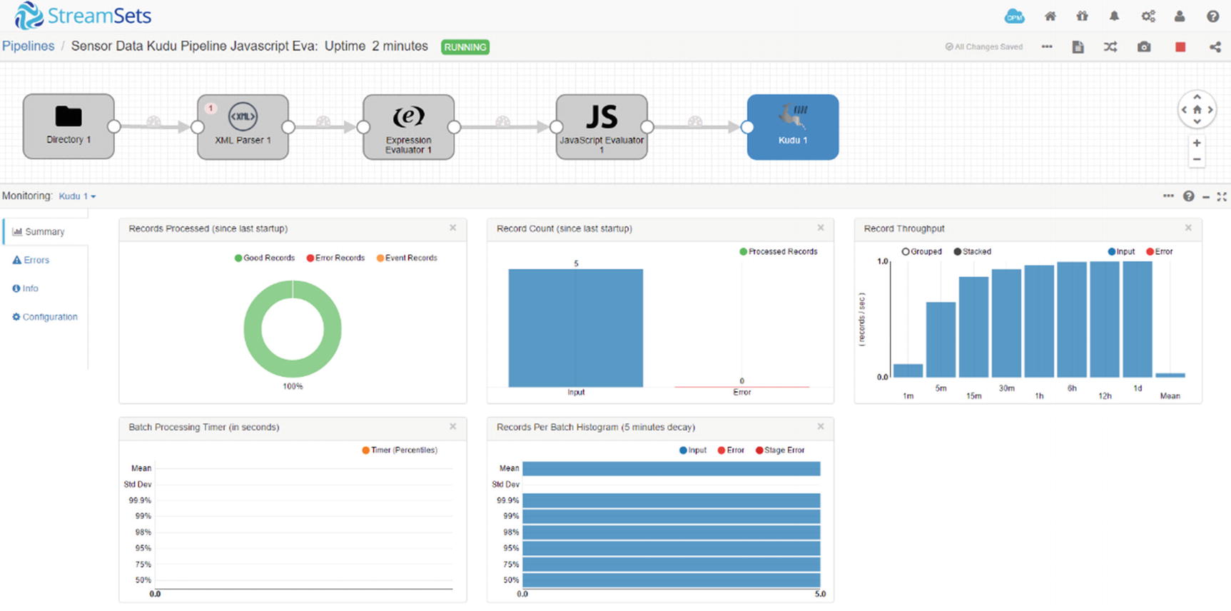
Monitor Kudu destination
Confirm that the data was successfully inserted to Kudu. As you can see, the action and uniqueid fields were successfully populated.
Congratulations! You’ve successfully used a JavaScript evaluator in your pipeline.
Ingesting into Multiple Kudu Clusters
Sometimes you’ll be required to ingest data into two or more active-active clusters for high availability and scalability reasons. With Data Collector this is easily accomplished by simply adding Kudu destinations to the canvas and connecting them to the processor. In this example, we will simultaneously ingest XML data into two Kudu clusters, kuducluster01 and kuducluster02.
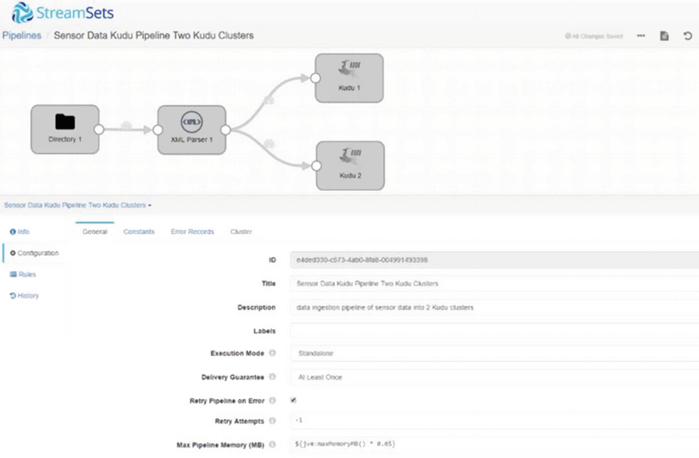
Multiple Kudu destinations
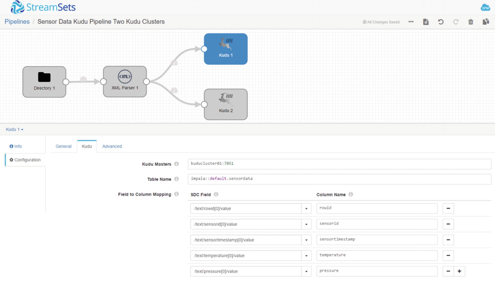
Configure first Kudu destination
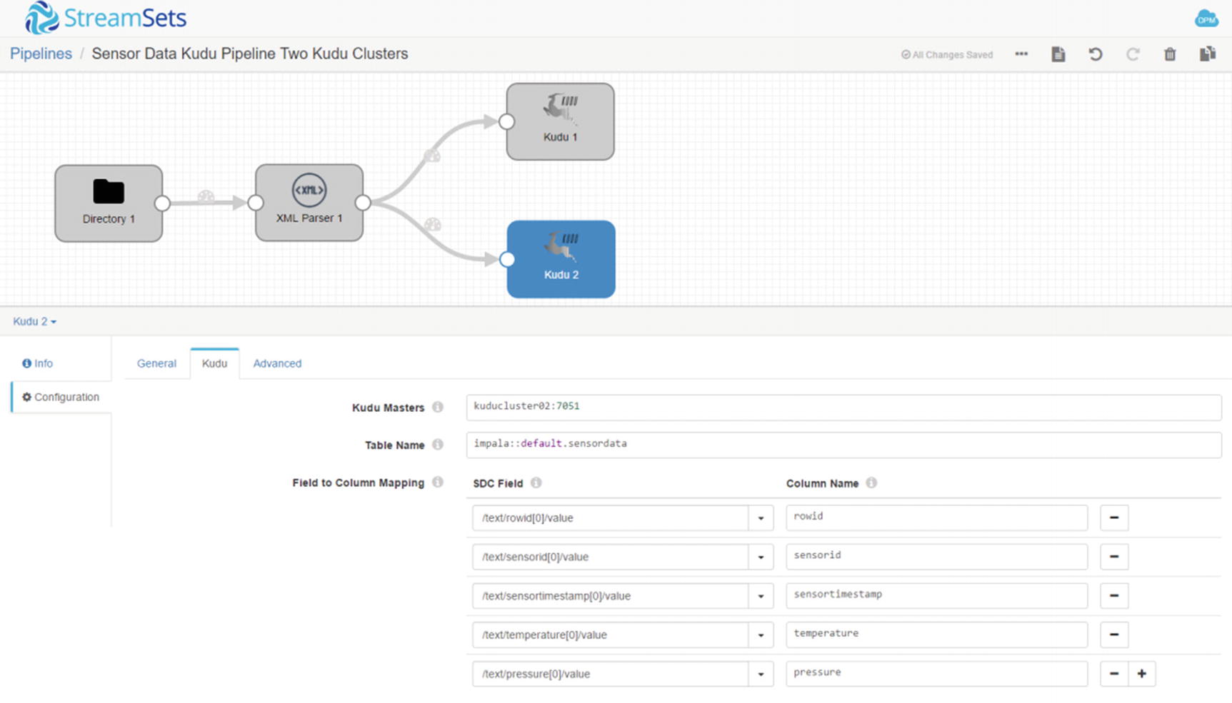
Configure second Kudu destination
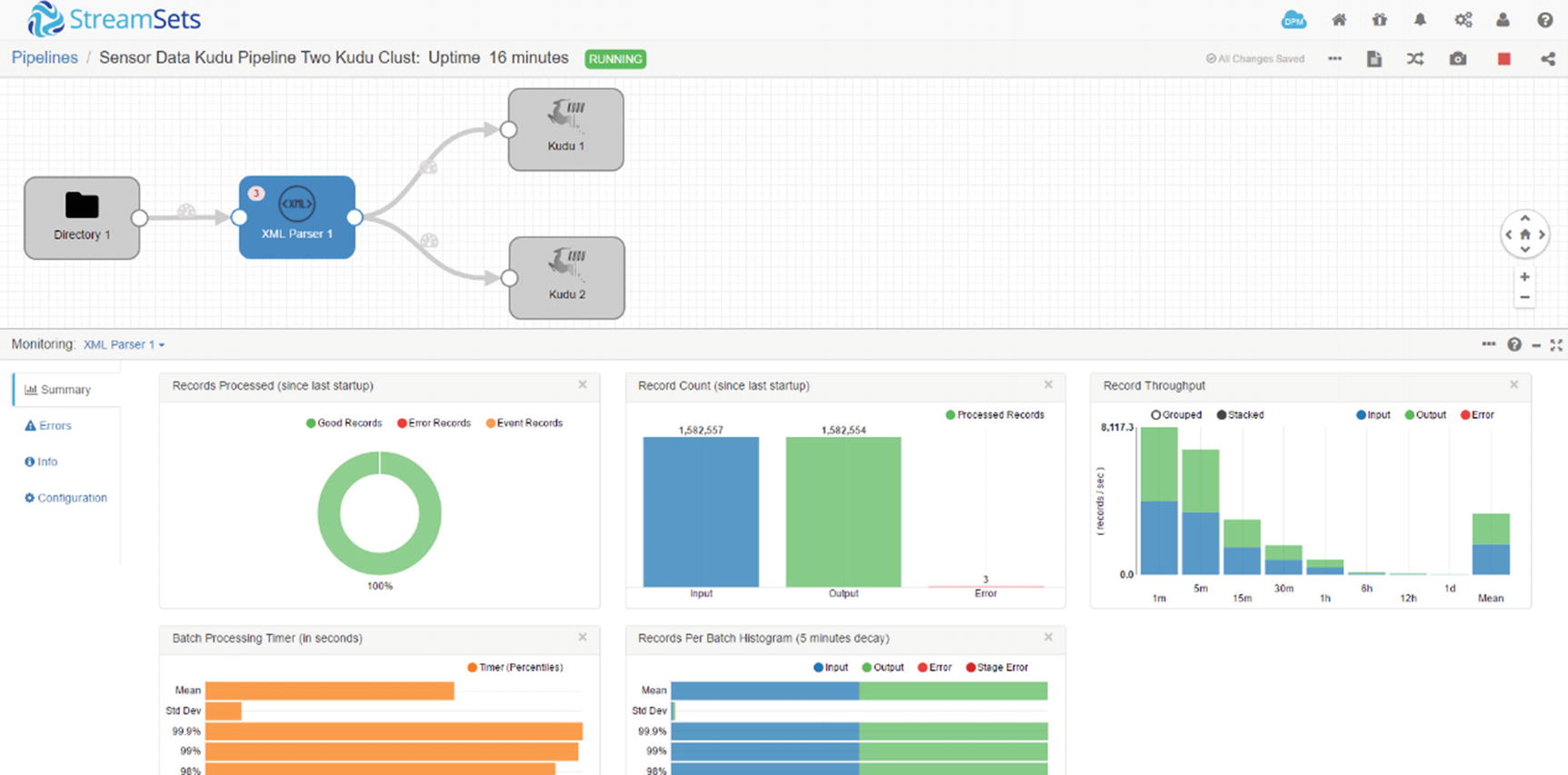
Monitor XML Parser
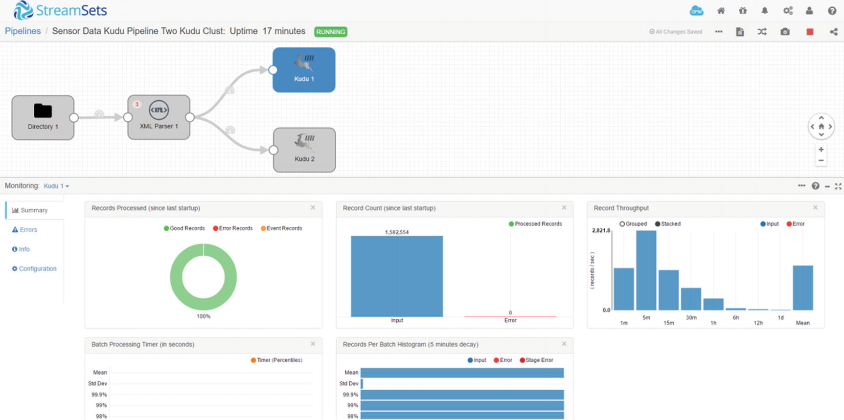
Monitor first Kudu destination
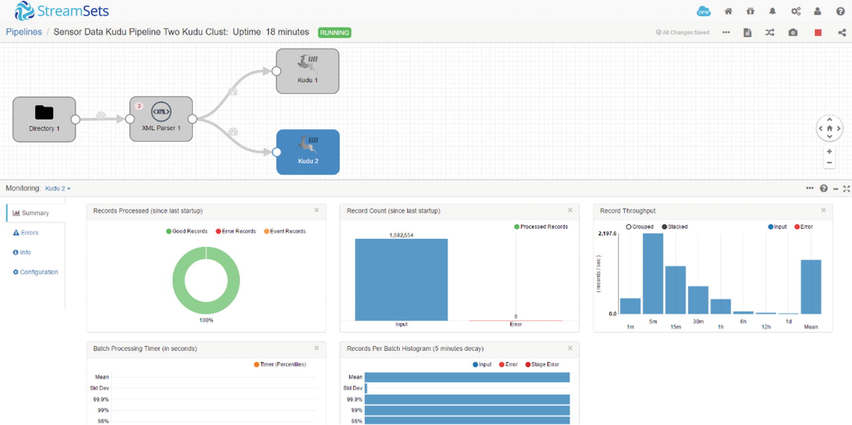
Monitor second Kudu destination
Verify in Impala. Perform a SELECT COUNT on the sensordata table on the first Kudu cluster.
Do the same SELECT COUNT on the second Kudu cluster.
You ingested data into two Kudu clusters simultaneously. You can ingest to different combinations of platforms such as HBase, Cassandra, Solr, Kafka, S3, MongoDB, and so on. Consult the Data Collector User Guide for more details.
REST API
Data Collector has an easy-to-use web-based GUI for designing, running, and administering pipelines. However, you can also use the built-in REST API if you’d like to programmatically interact with Data Collector, for automation purposes, for example. xviii The REST API lets you access all aspects of Data Collector, from starting and stopping pipelines, returning configuration information and monitoring pipeline metrics.
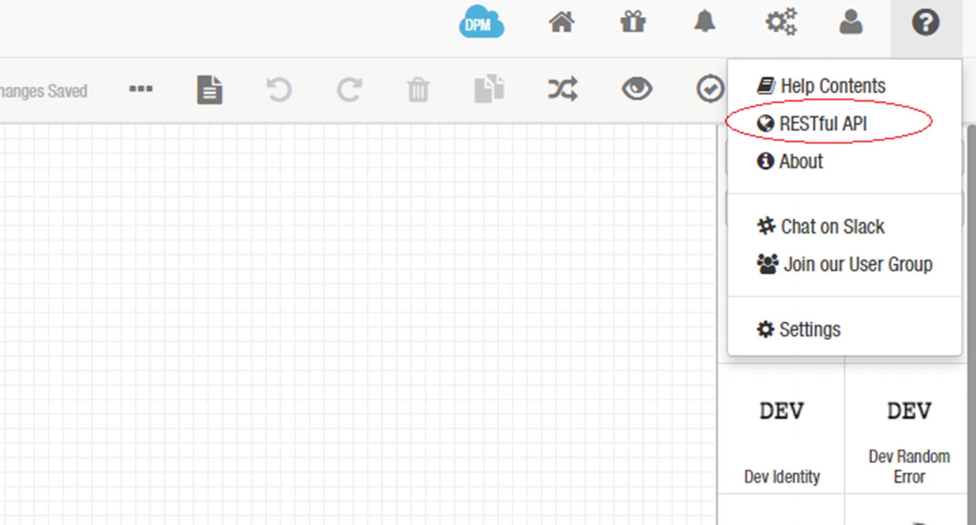
REST API
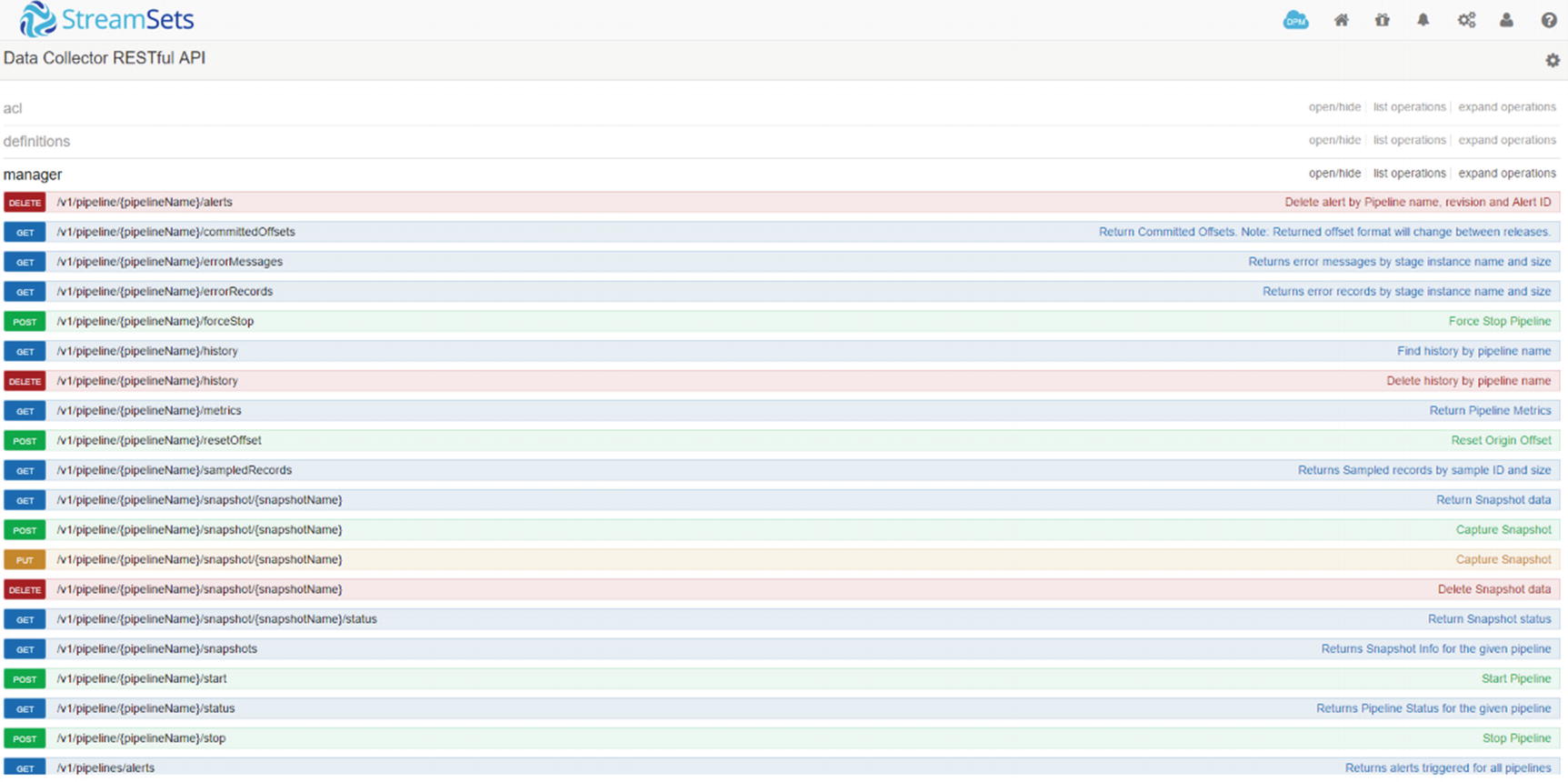
List of available operations
Expand “Return All Pipeline Status.” Choose the response content type “application/json” and click the “try it out” button.
The “response body” will contain details about your pipelines in JSON format similar to Listing 7-2. Depending on the number of pipelines and type of error messages returned, the response body could be quite large.
Return all pipeline status response body
You can make REST API requests by using curl, a utility that can download data using standard protocols. The username and password and Custom HTTP header attribute (X-Requested-By) are required.
Event Framework
StreamSets has an Event Framework that allows users to kick off tasks in response to triggers or events that happen in the pipeline. StreamSets uses dataflow triggers to execute tasks such as send e-mails, execute a shell script, starting a JDBC query, or starting a Spark job after an event, for example, after the pipeline successfully completes a JDBC query.
Dataflow Performance Manager
One of the most powerful feature of StreamSets is StreamSets Dataflow Performance Manager. StreamSets Dataflow Performance Manager (DPM) is a management console that lets you manage complex data flows, providing a unified view of all running pipelines in your environment. DPM is extremely helpful in monitoring and troubleshooting pipelines. You’ll appreciate its value more when you’re tasked to monitor hundreds or even thousands of pipelines. Covering DPM is beyond the scope of this book. For more information, consult the Data Collector User Guide.
I’ve only covered a small subset of StreamSets features and capabilities. For more information about StreamSets, consult the StreamSets Data Collector User Guide online. In Chapter 9, I use StreamSets, Zoomdata , and Kudu to create a complete Internet of Things (IoT) application that ingests and visualizes sensor data in real time.
Other Next-Generation Big Data Integration Tools
There are other next-gen data integration tools available in the market. I discuss some of the most popular options in the Cask Data Application Platform.
The Cask Data Application Platform (CDAP) is an open source platform that you can use to develop big data applications and ETL jobs using Spark and the Hadoop stack. CDAP provides a GUI-based data ingestion studio for developing, deploying, and administering data pipelines. Its data preparation features provide an interactive method for data cleansing and transformation, a set of tasks commonly known as data wrangling. CDAP also has an application development framework, high-level Java APIs for rapid application development, and deployment. On top of that, it has metadata, data lineage, and security features that are important to enterprise environments. Like StreamSets, it has native support for Kudu. Let’s develop a CDAP pipeline to ingest data to Kudu.
Data Ingestion with Kudu
The first thing we need to do is prepare test data for our example.

CDAP welcome page
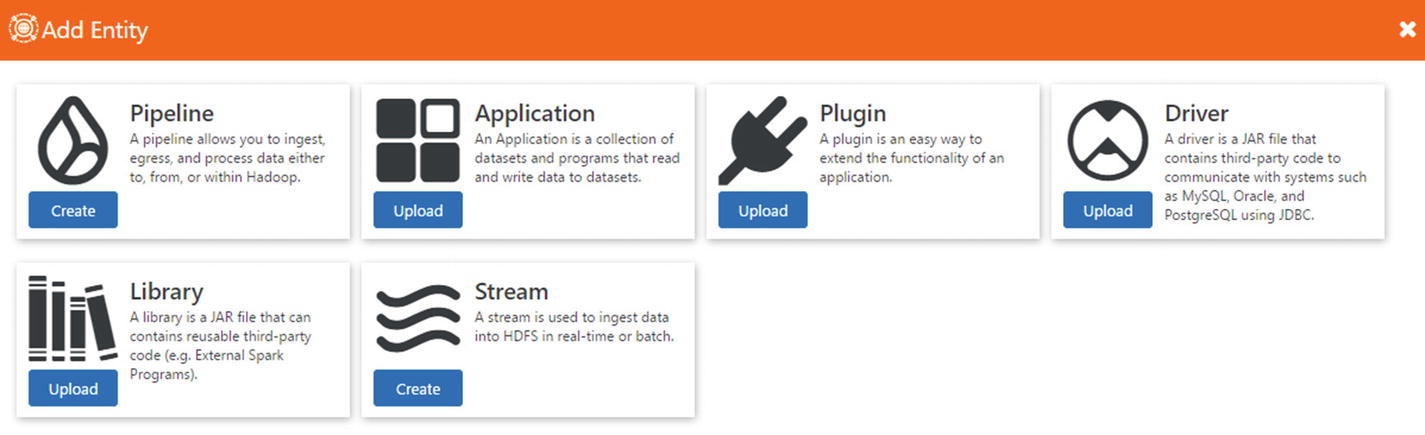
Add Entity
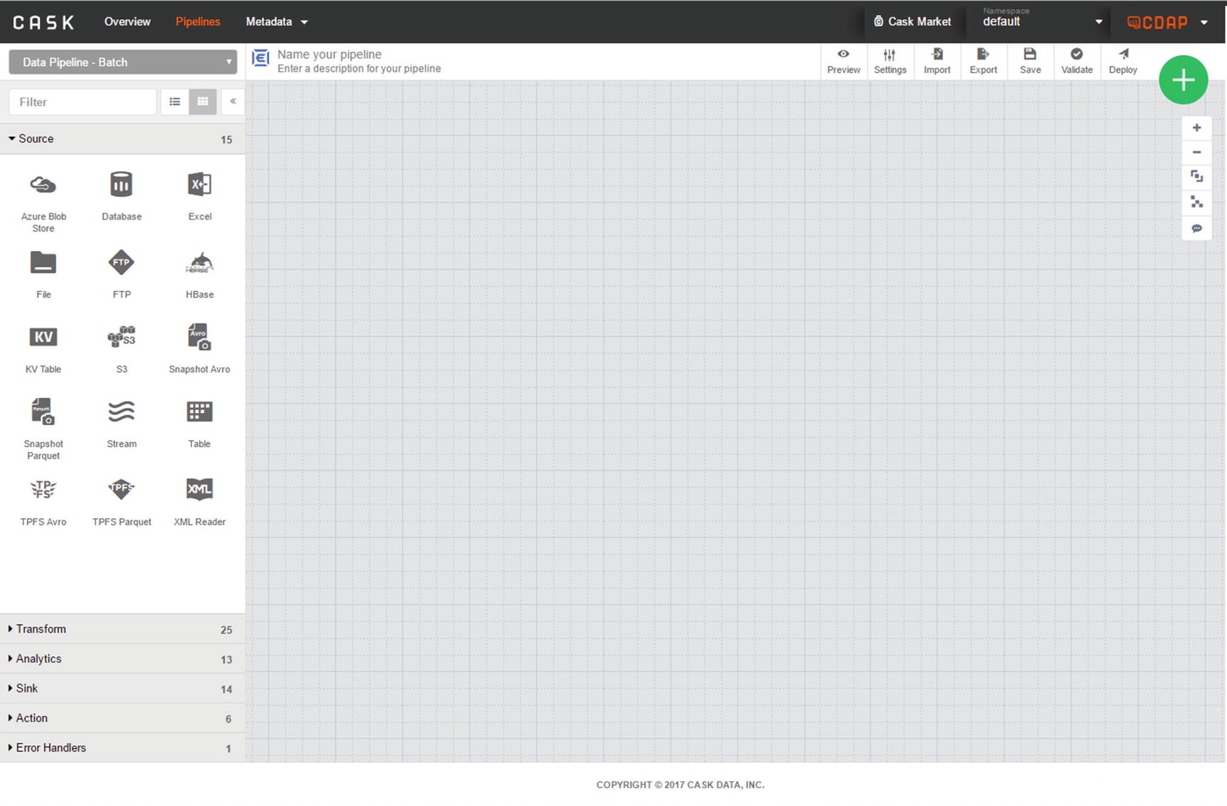
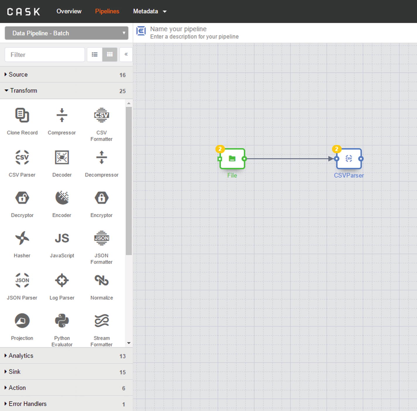
CDAP canvas
You may notice that the Kudu source and sink are missing. We need to add the Kudu source and sink from the Cask Market. Click the “Cask Market” link near the upper-right corner of the application window.
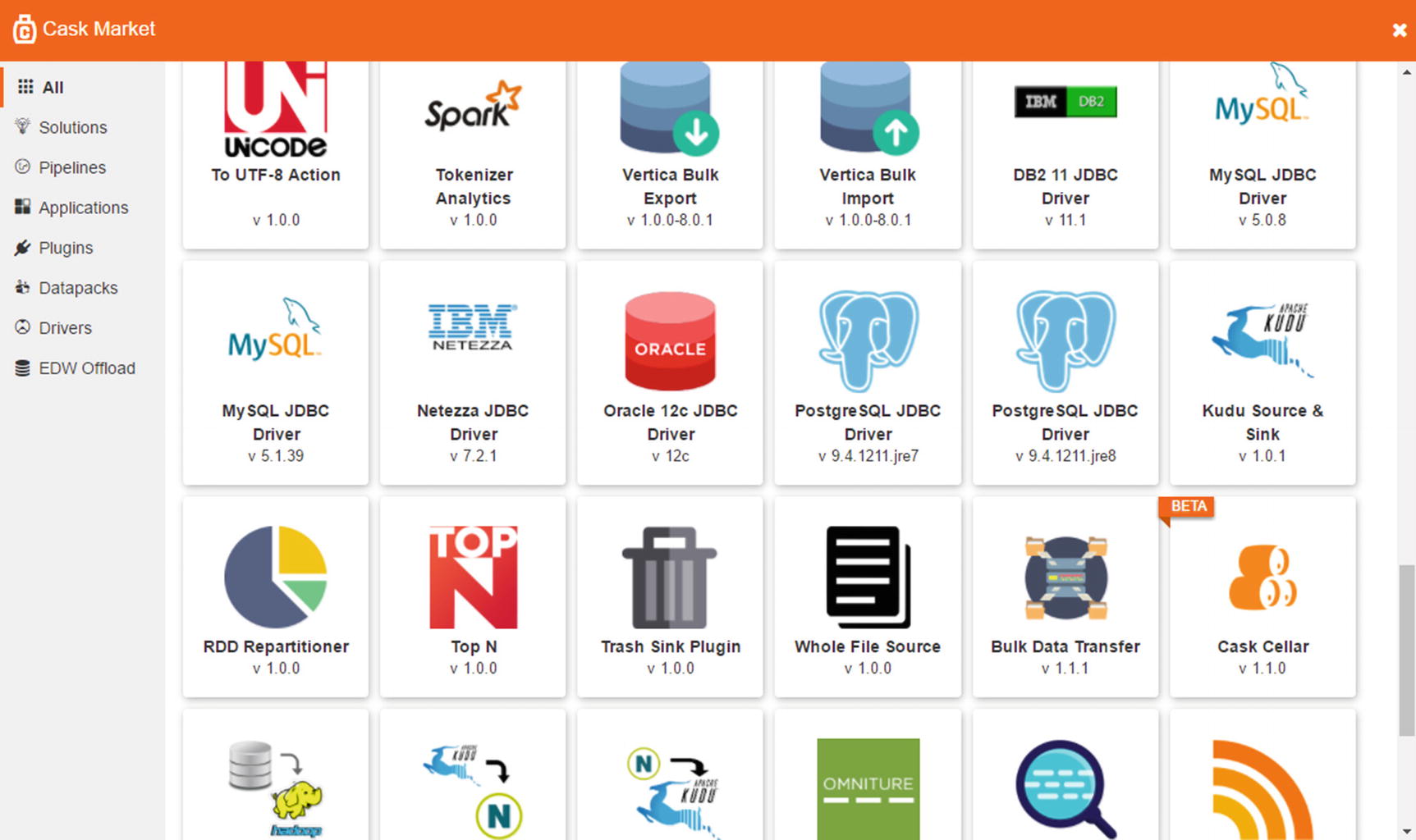
Cask Market
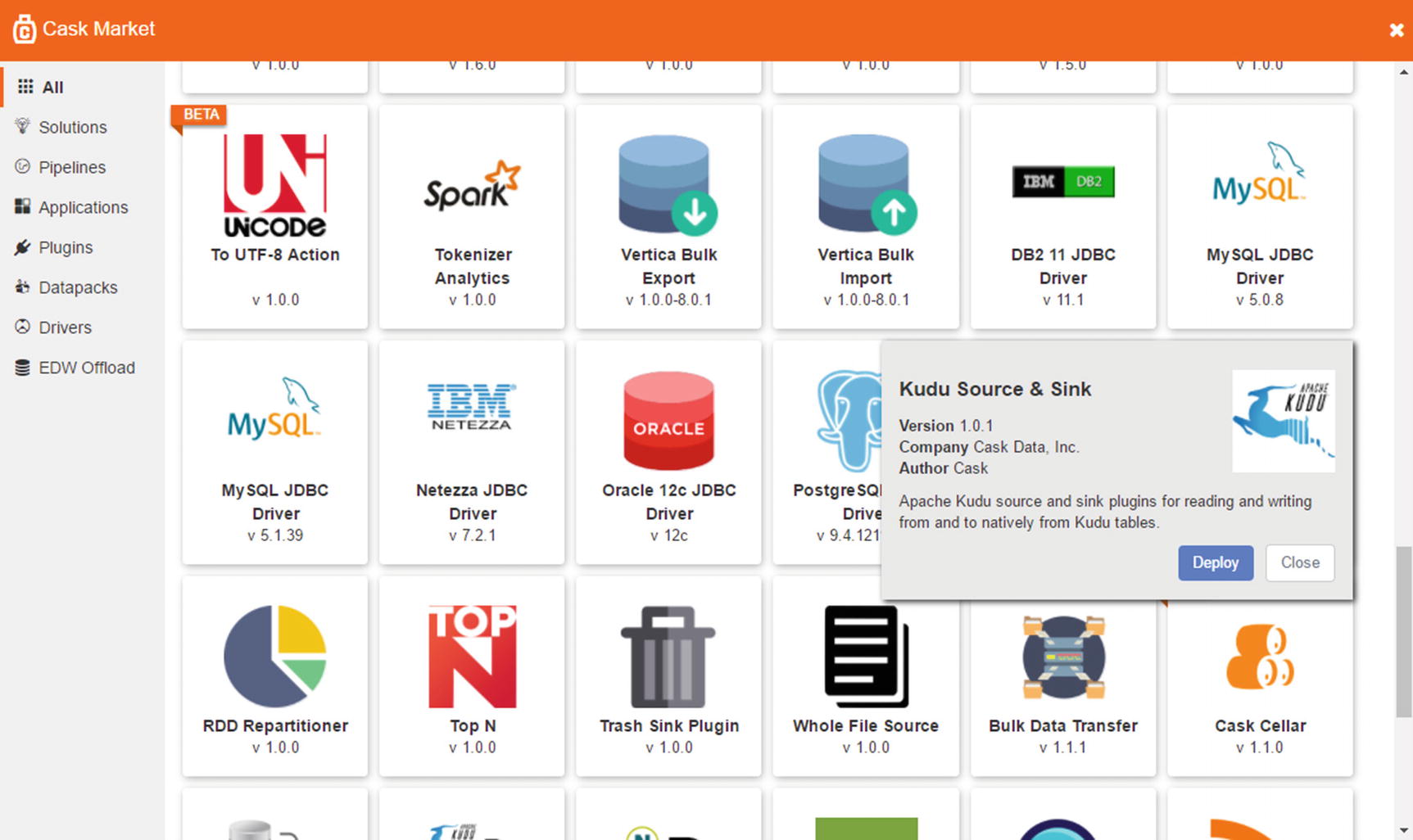
Cask Market – Kudu Source and Sink
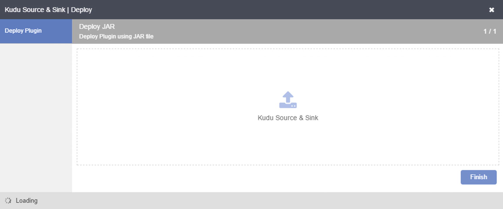
Finish installation
Kudu data source and sink
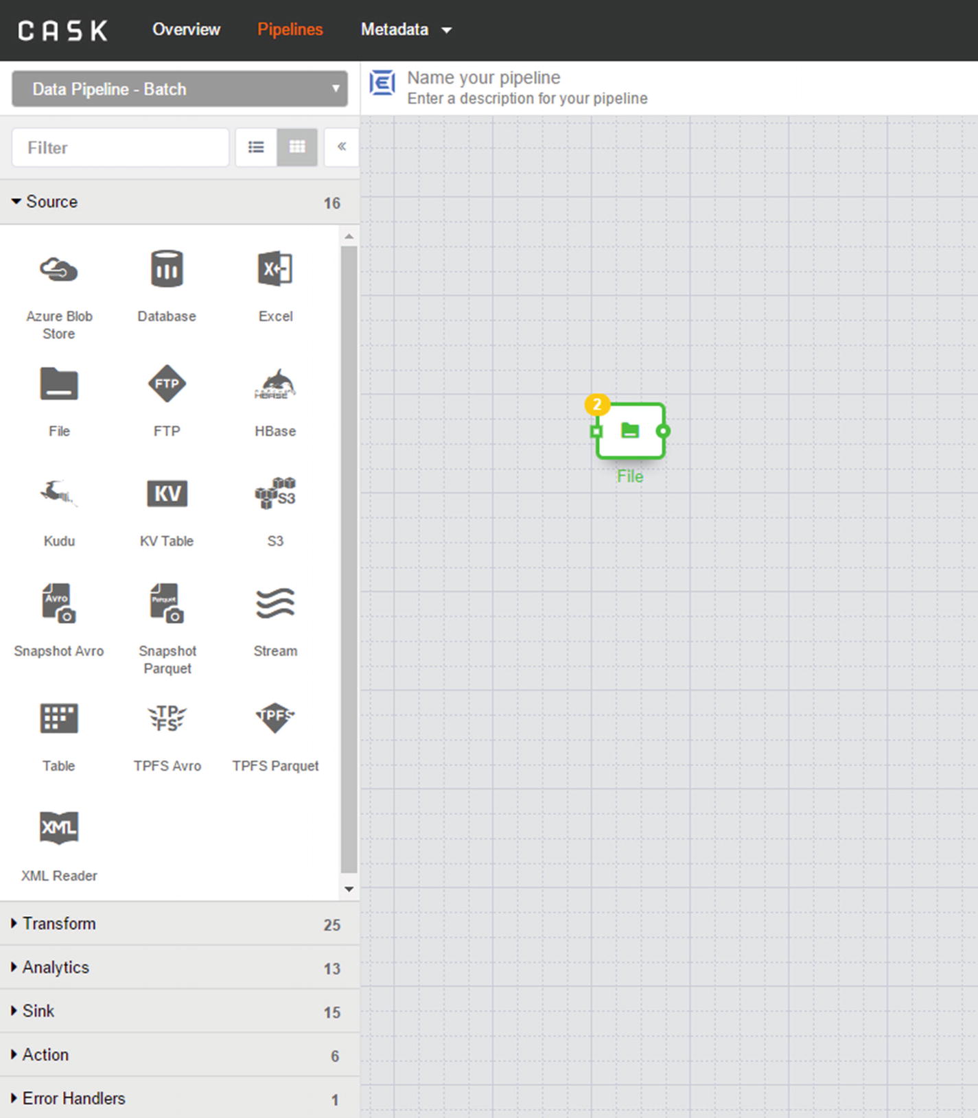
File source
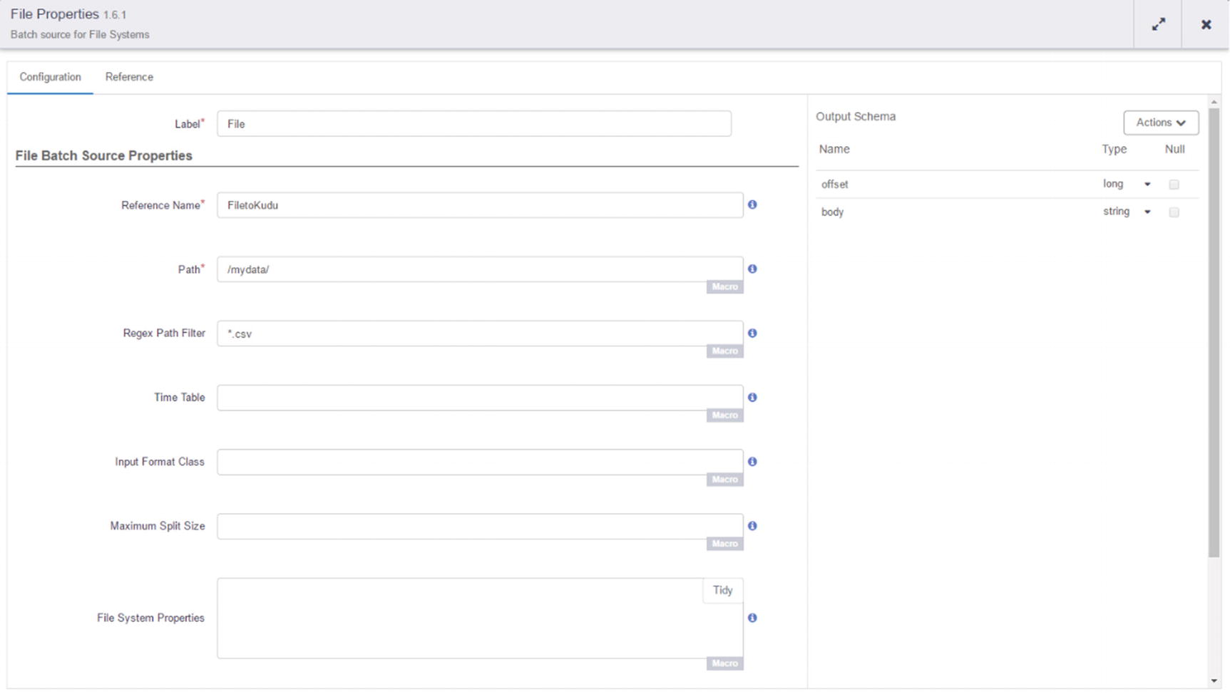
File properties
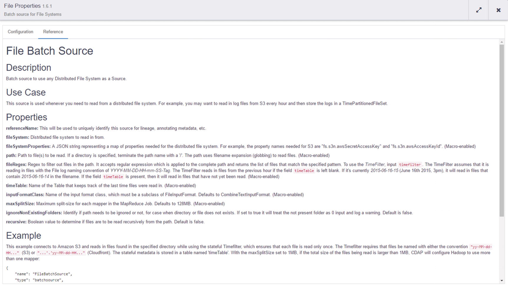
File Batch Source documentation
CSVParser transformation
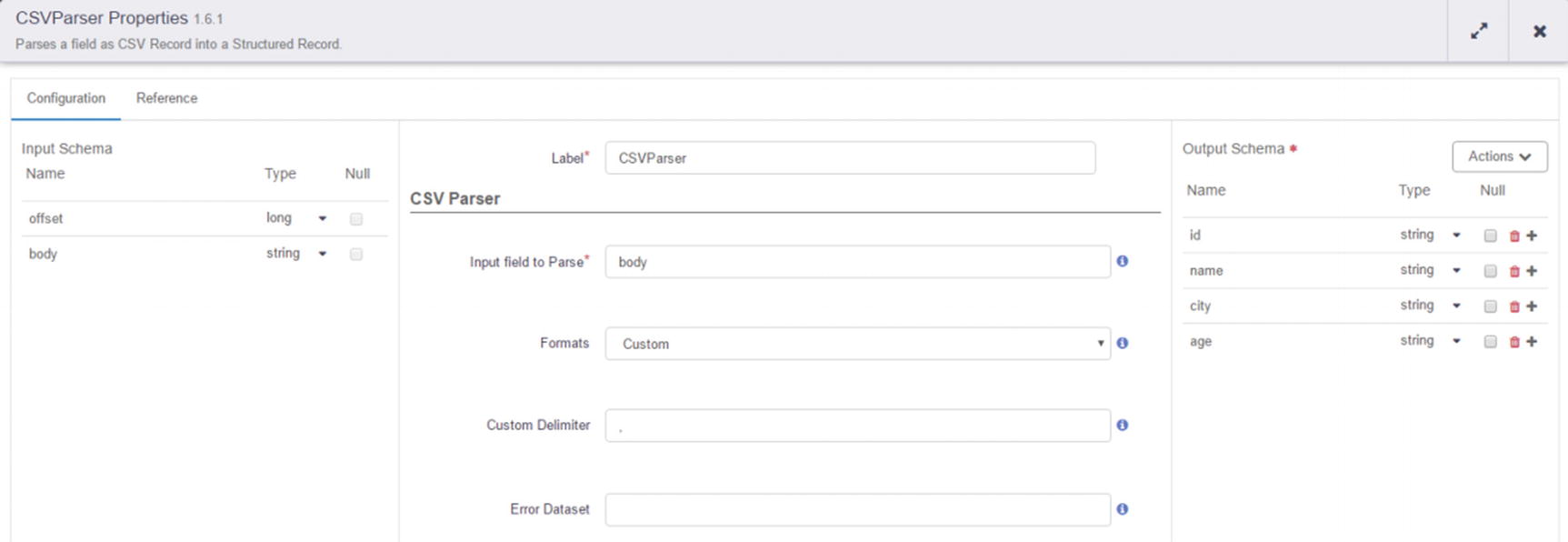
Configure CSVParser
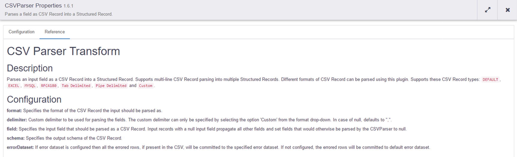
CSVParser documentation
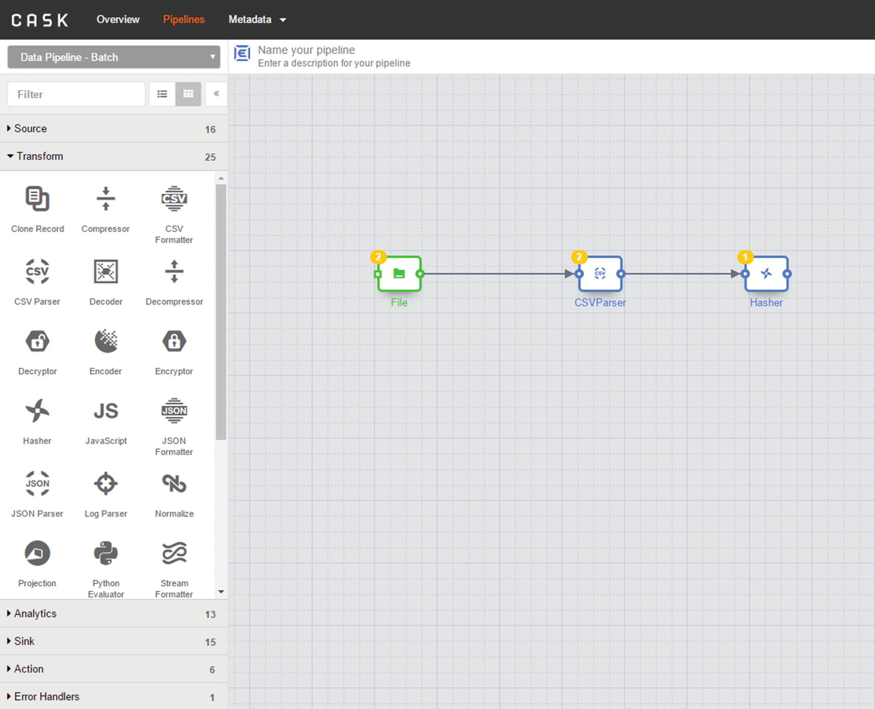
Hasher transformation
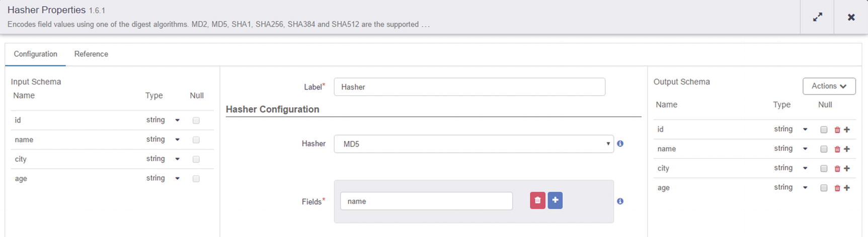
Hasher configuration
Kudu sink
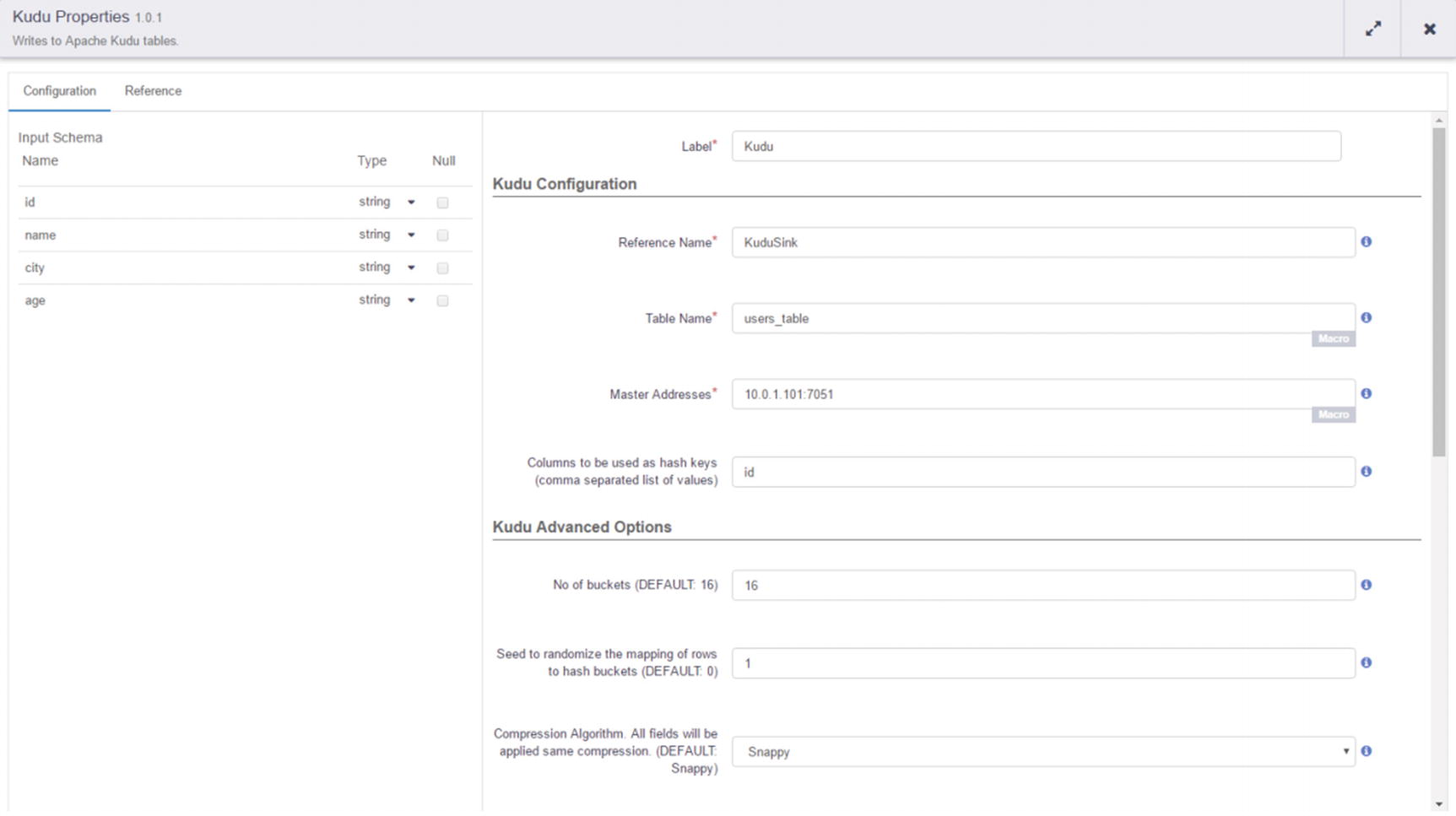
Kudu sink configuration
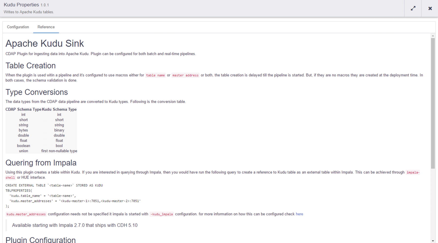
Kudu sink documentation
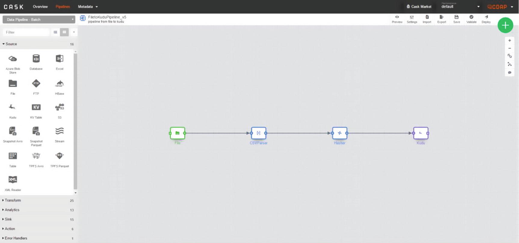
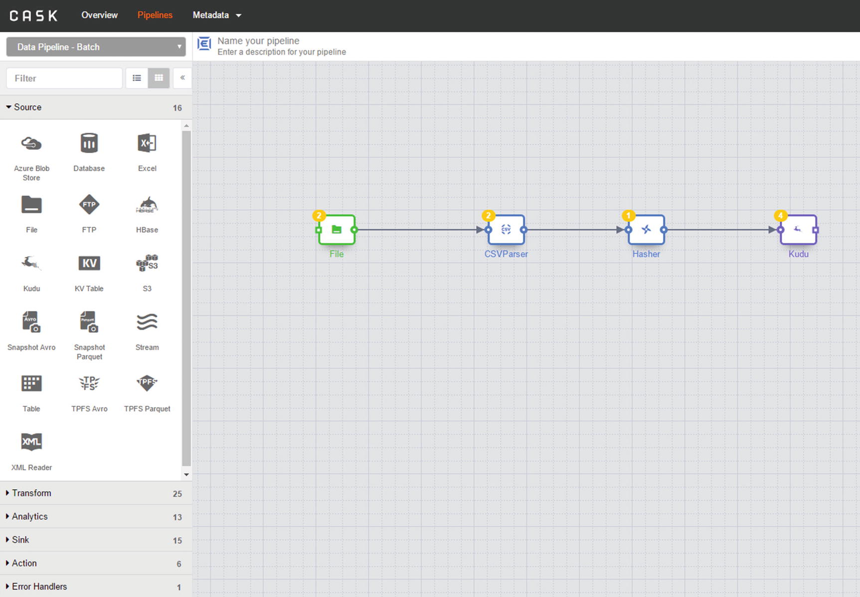
Complete pipeline

Number of records transferred and processed
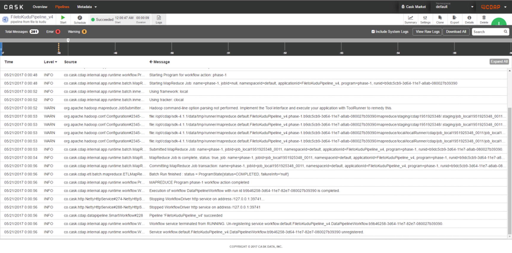
Check CDAP logs
Confirm that the rows were successfully inserted to the Kudu table. First, we have to create an external table in Impala on top of the Kudu table that CDAP created. Make sure the name field is hashed.
You’ve successfully ingested data into a Kudu table, using a Field Hasher to perform in-stream transformation to your data.
Pentaho Data Integration
Pentaho offers a complete line of products for data integration, big data processing, and business analytics. We’ll focus on Pentaho Data Integration (PDI) in this chapter. There is a community version called Pentaho Community Edition (CE), which includes Kettle, the open source version of Pentaho Data Integration. There is an Enterprise version, which includes Native YARN integration, analyzer and dashboard enhancements, advanced security, and high availability features. xix
Pentaho PDI has an intuitive user interface with ready-built and easy-to-use components to help you develop data ingestion pipelines. Similar to most ETL tools in the market, Pentaho PDI allows you to connect to different types of data sources ranging from popular RDBMS such as Oracle, SQL Server, MySQL, and Teradata to Big Data and NoSQL platforms such as HDFS, HBase, Cassandra, and MongoDB. PDI includes an integrated enterprise orchestration and scheduling capabilities for coordinating and managing workflows. You can effortlessly switch between Pentaho’s native execution engine and Apache Spark to scale your pipelines to handle large data volumes.
Ingest CSV into HDFS and Kudu
Unlike other data integration tools described in this chapter, Pentaho does not include native support for Kudu yet. In order for us to insert data into Kudu, we will need to use Pentaho’s generic Table Output component using Impala’s JDBC driver. Using Table Output directly may not be fast enough depending on the size of your data and data ingestion requirements. One way to improve performance is to stage data to HDFS first, then using Table Output to ingest data from HDFS to Kudu. In some cases, this may be faster than directly ingesting into Kudu.
The first thing we need to do is prepare test data for our example.
Start Pentaho Data Integration
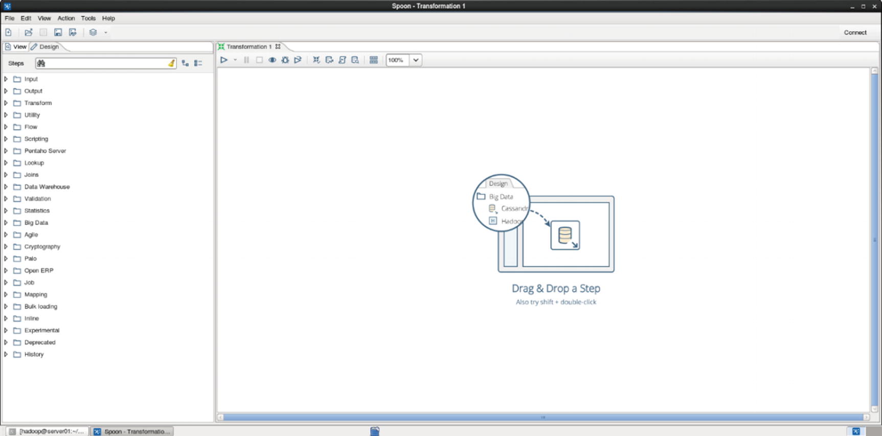
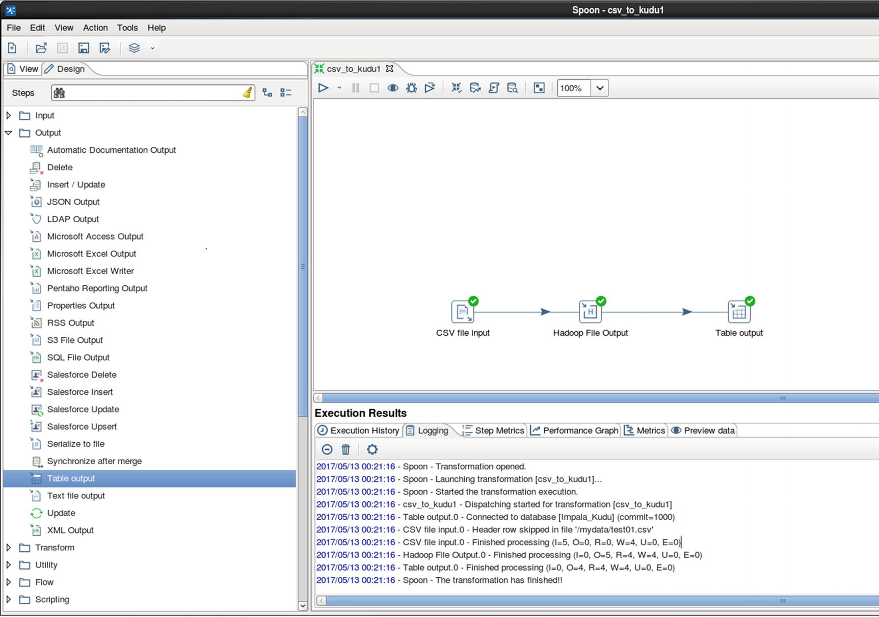
Graphical view
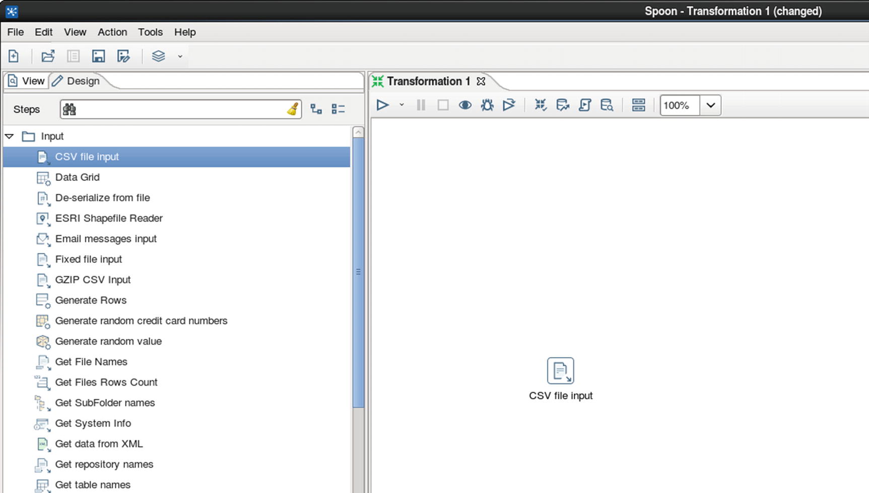
CSV file input
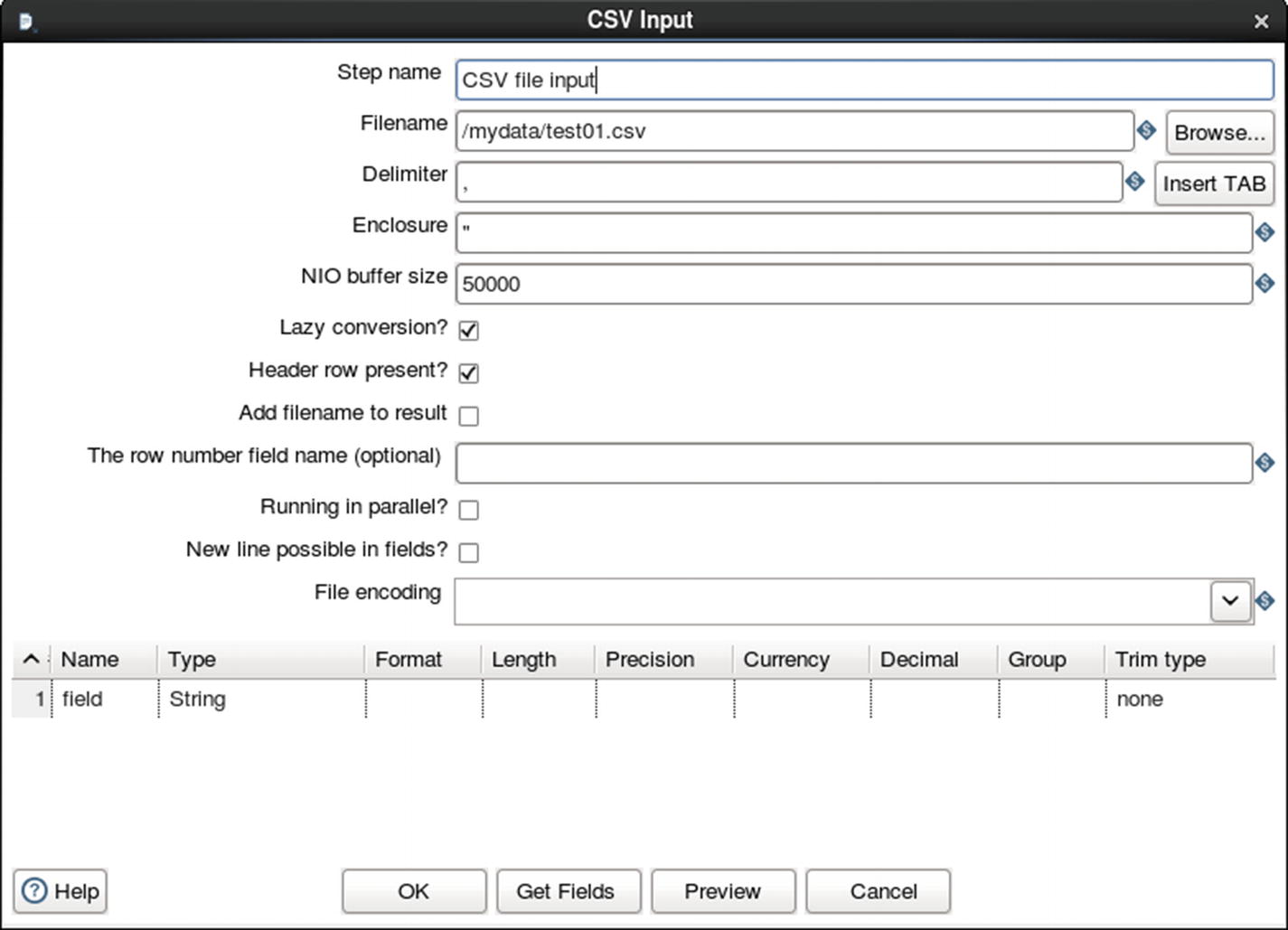
Configure CSV file input
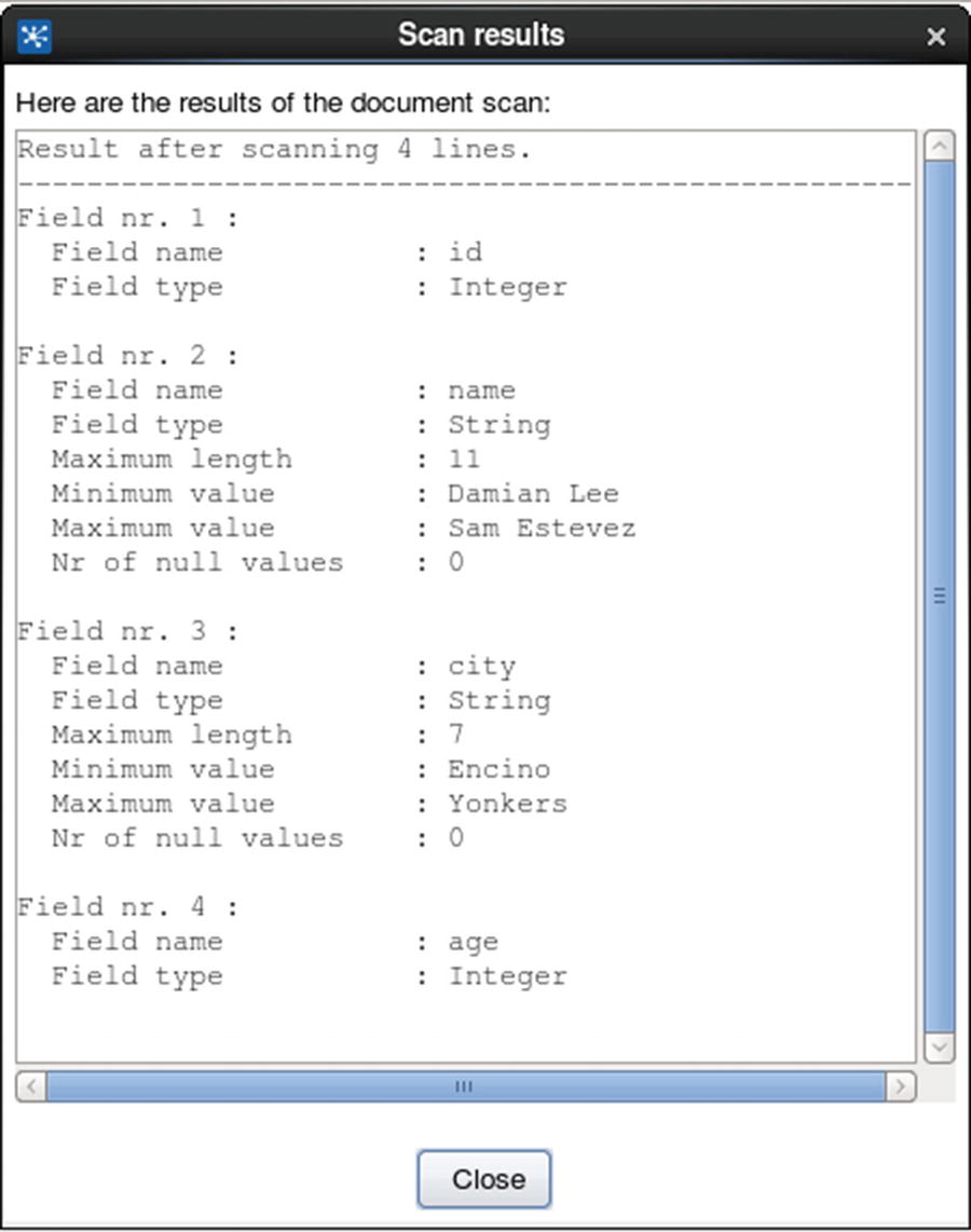
Get fields
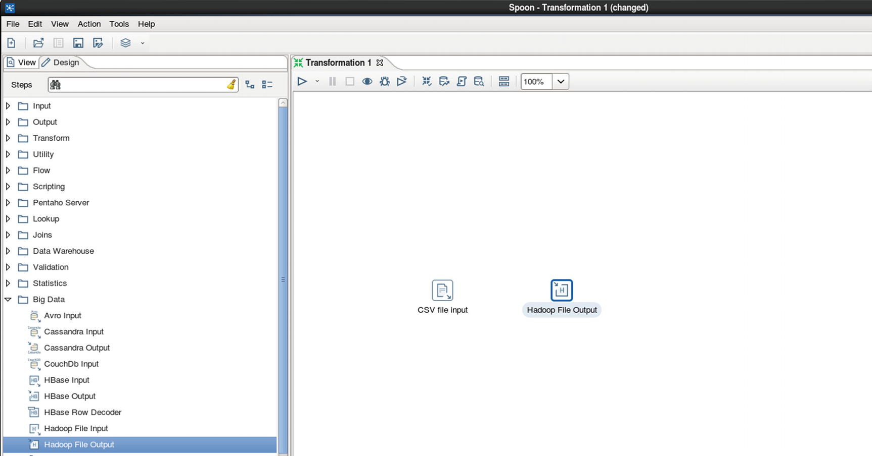
Hadoop file output
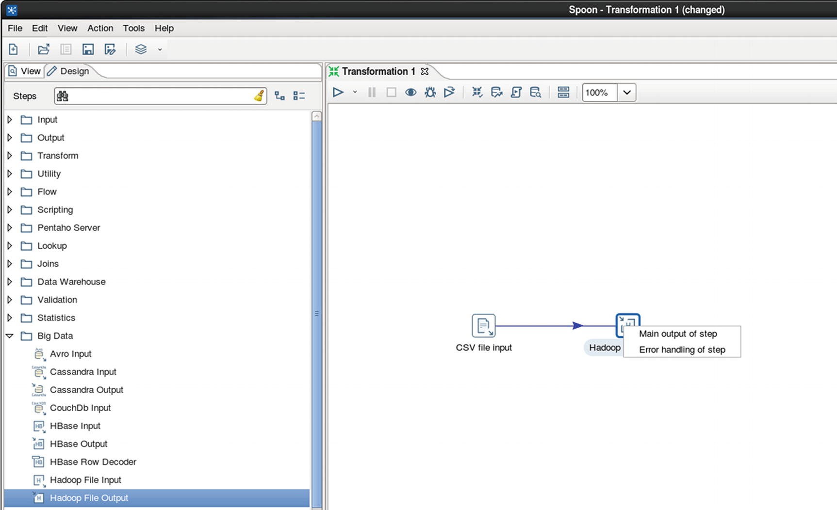
Connect CSV file input to Hadoop file output
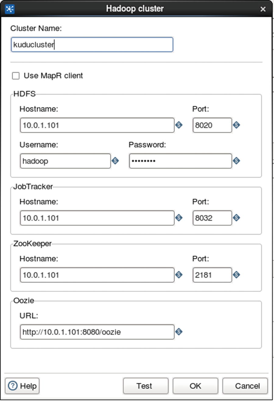
Configure Hadoop file output
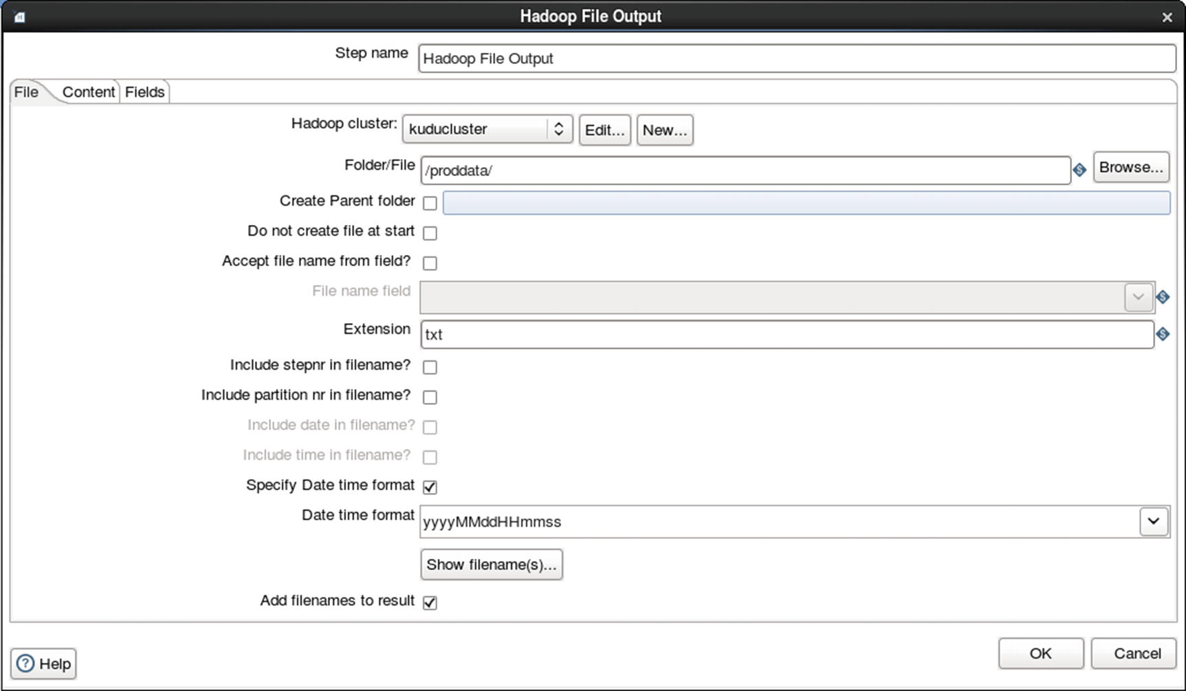
Rename file based on date time format
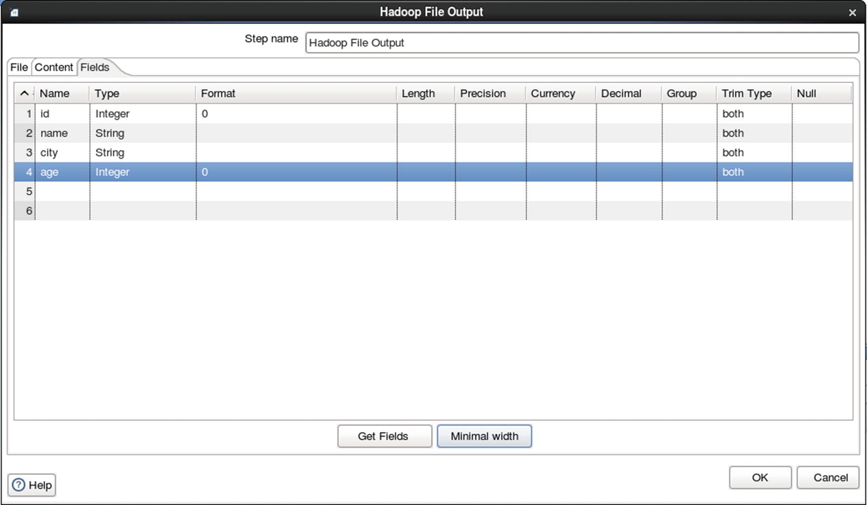
Configure fields
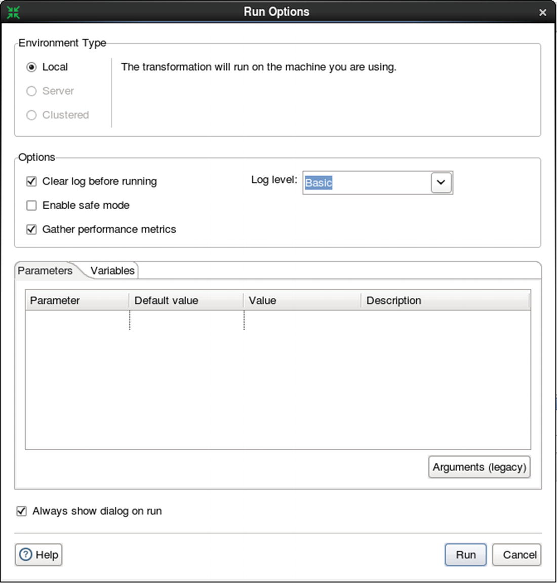
Run the job
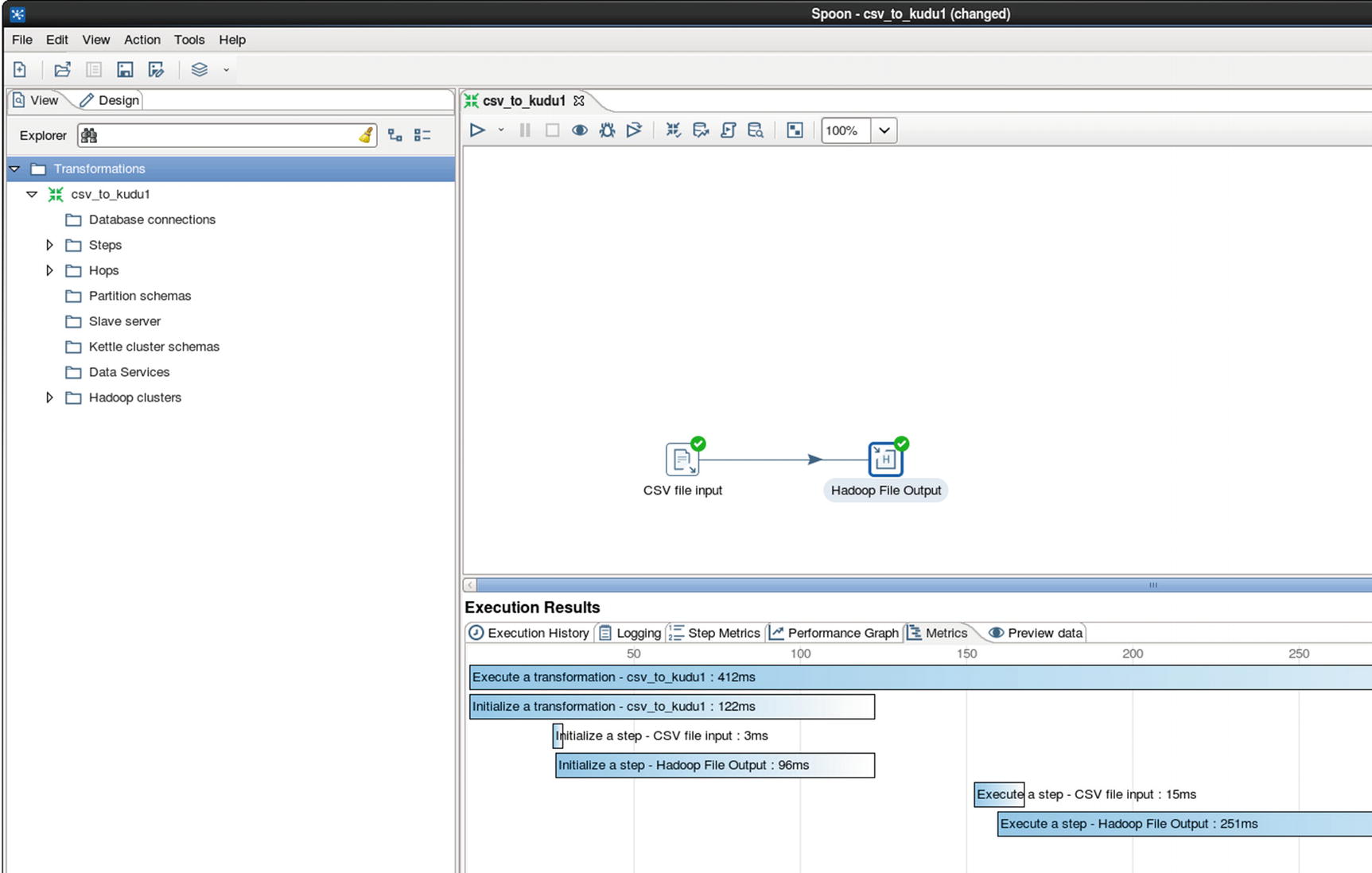
Execution Results
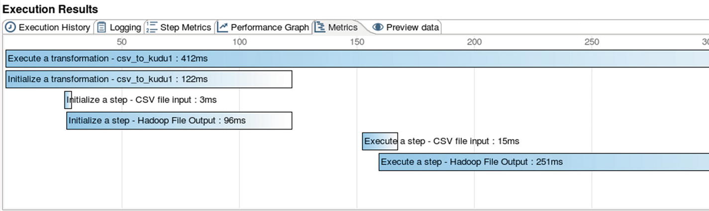
Metrics – Execution Results
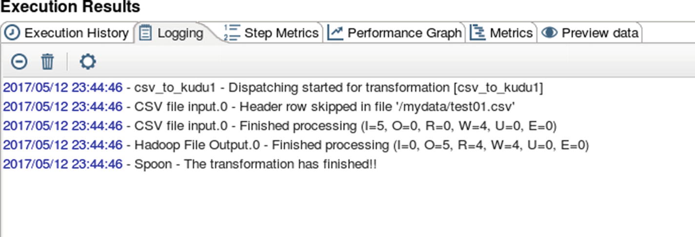
Logging – Execution Results
Confirm that the file was indeed copied to HDFS.
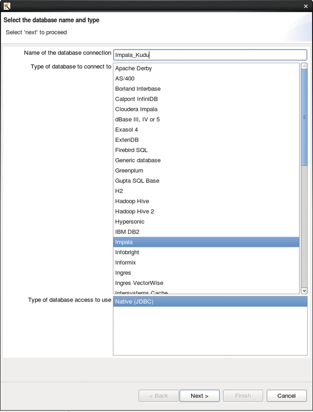
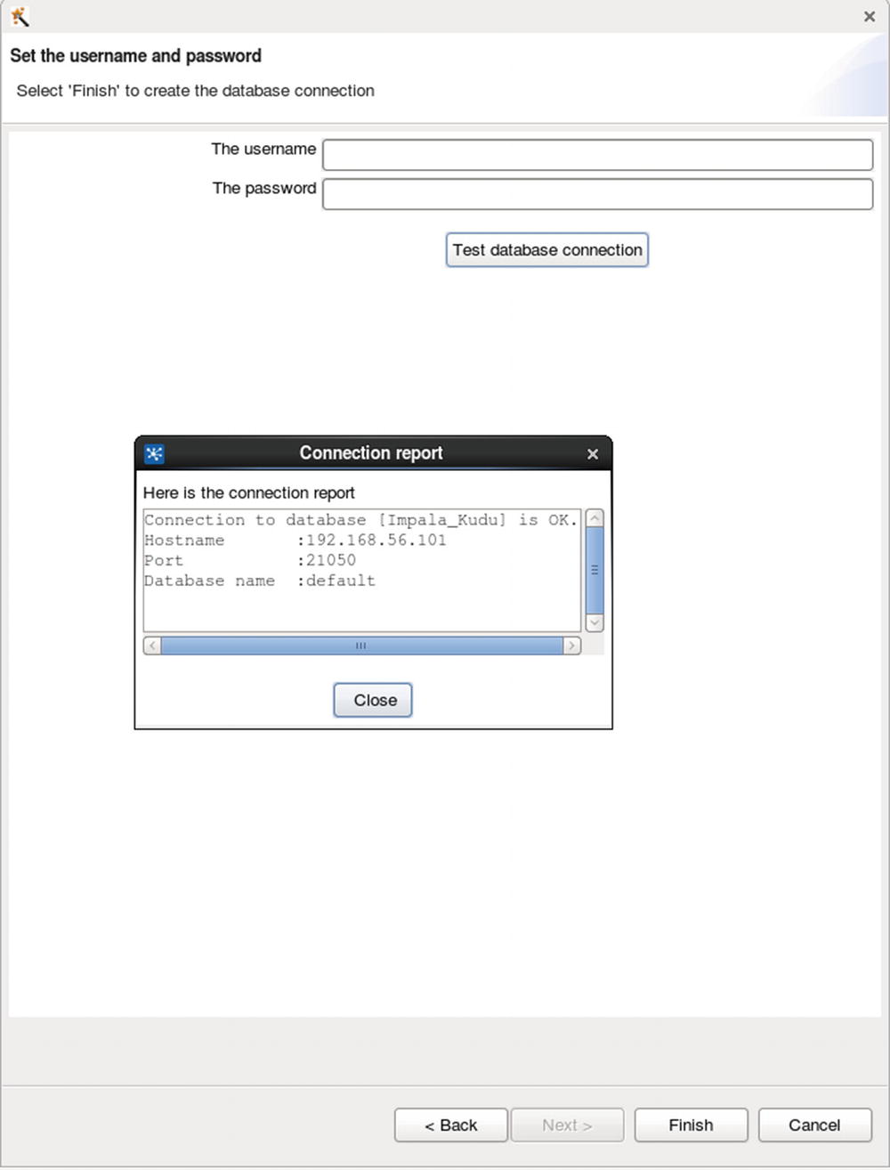
Configure database connection
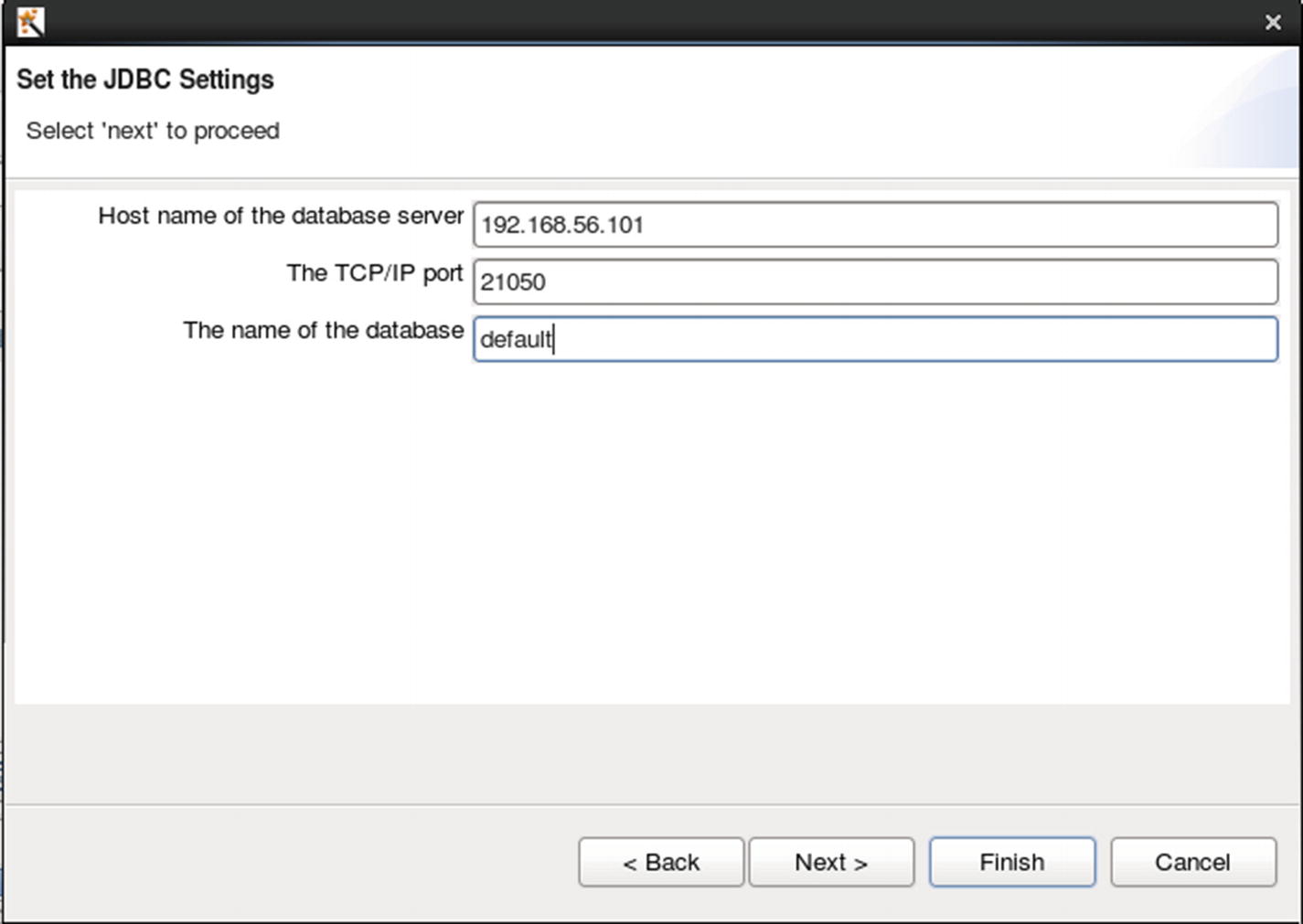
Configure JDBC settings
Create the destination table.
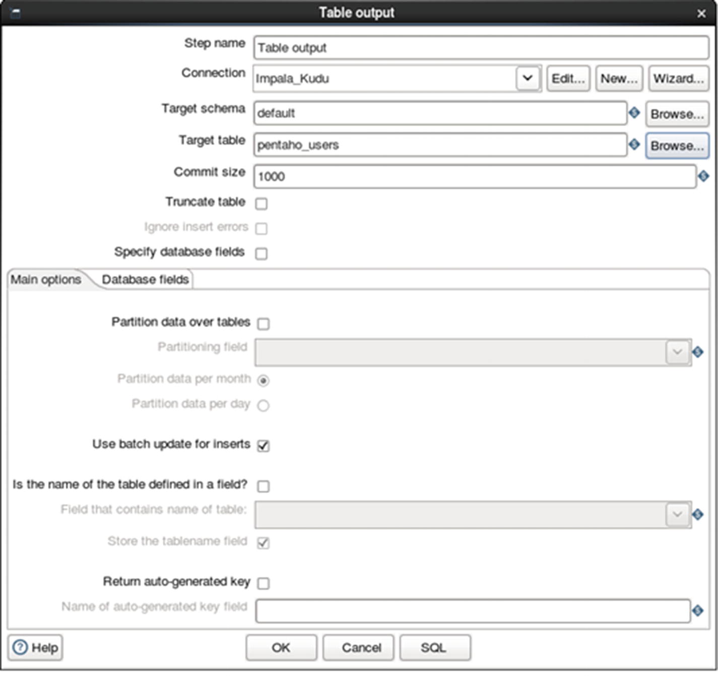
Configure table output
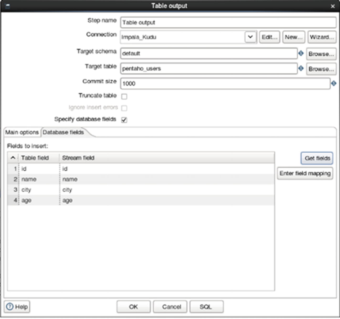
Get fields
Run the job
The job ran successfully.
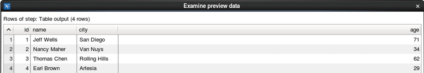
Confirm that the data was successfully inserted into the Kudu table.
Data Ingestion to Kudu with Transformation
Let’s start with another example. This time we’ll use a string replace transformation to replace the string “Yonkers” with “Berkeley.”
Prepare the data.
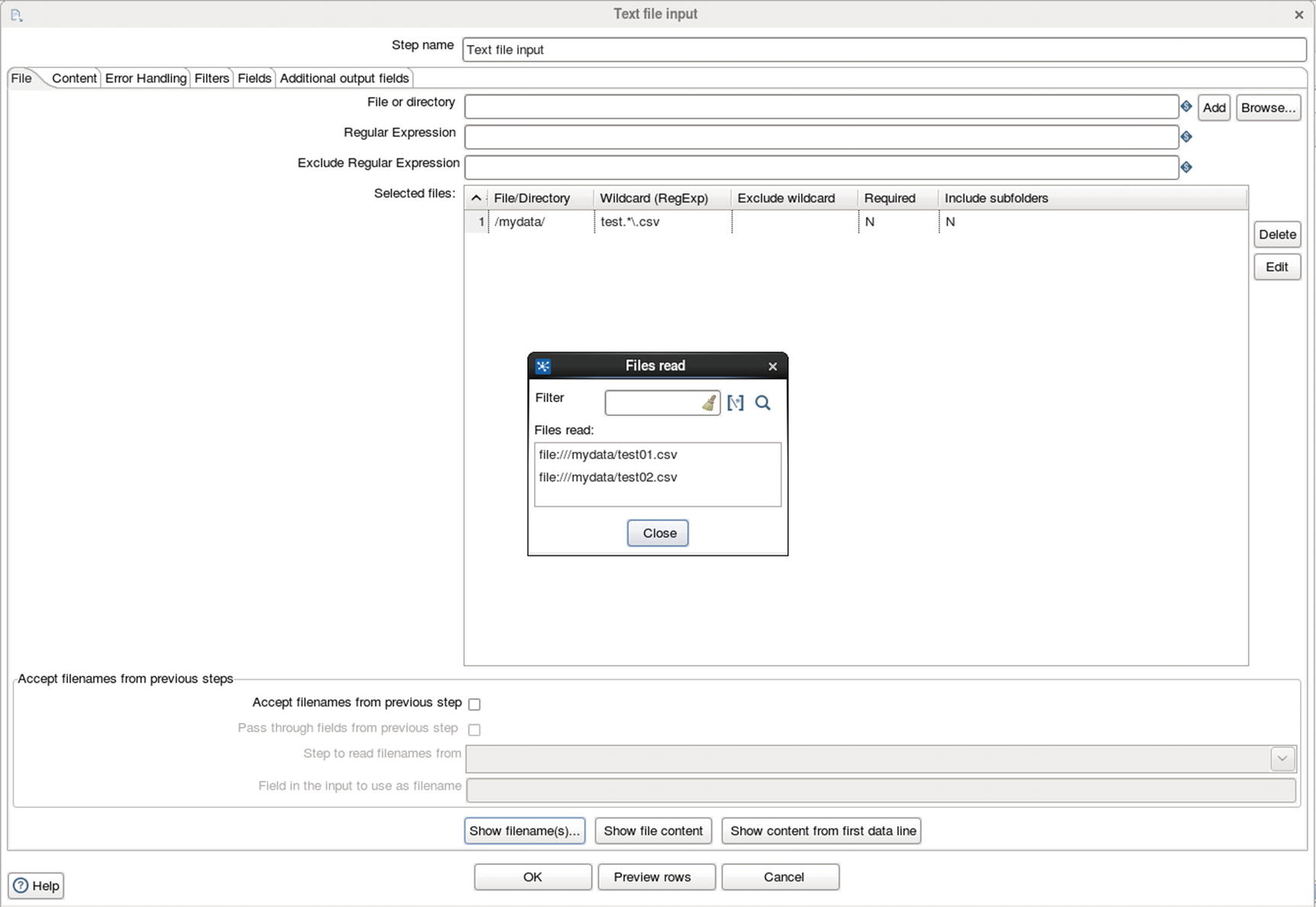
Specify source directory and file
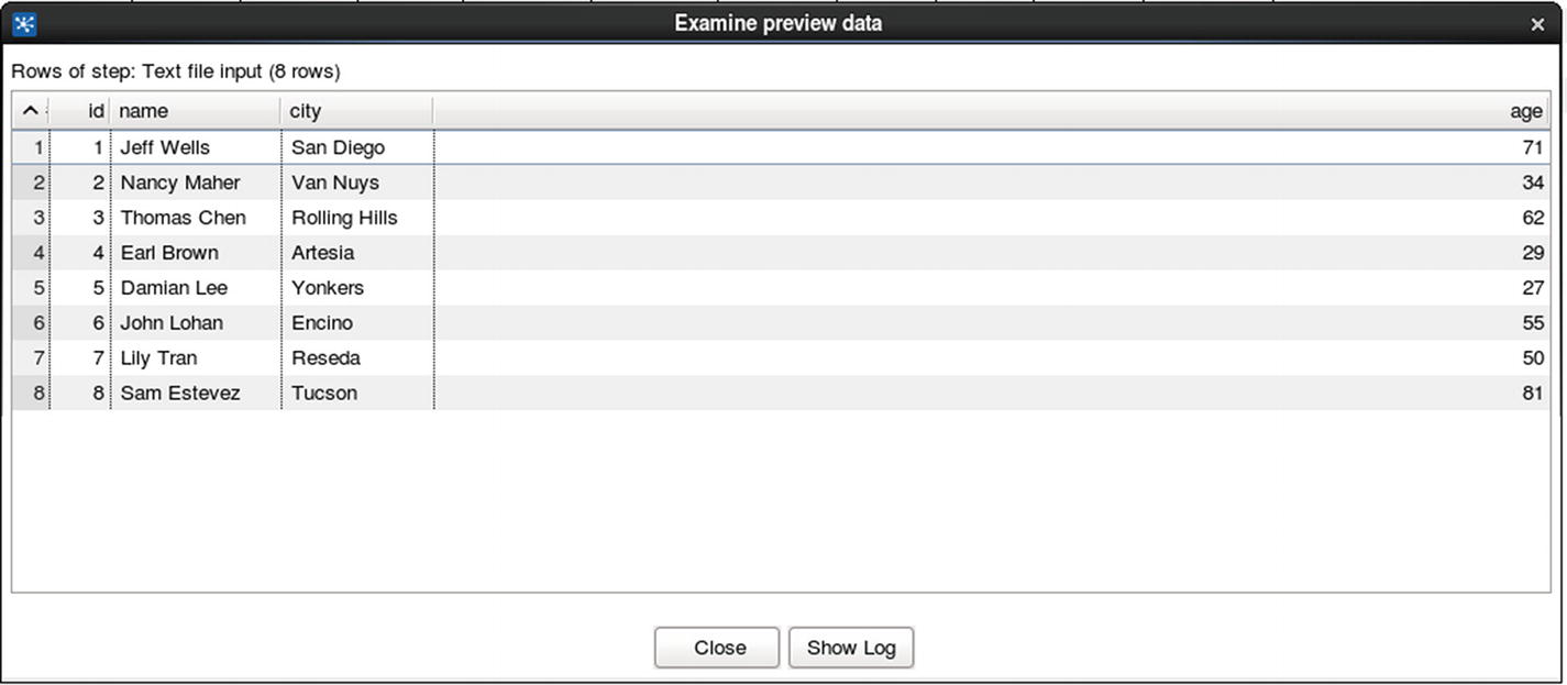
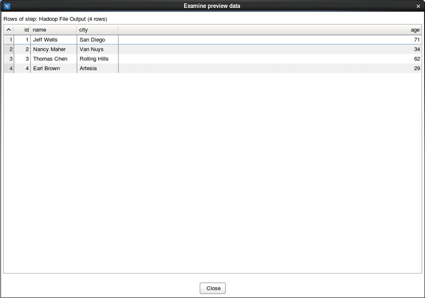
Preview data
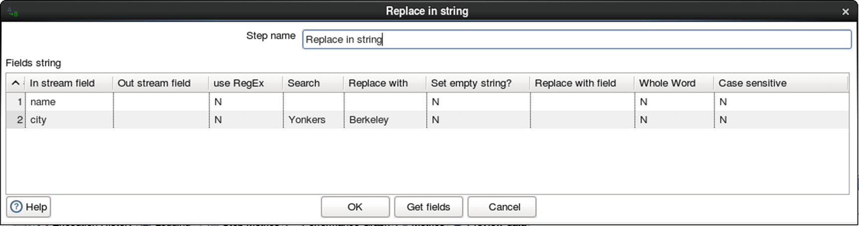
Replace a string transformation
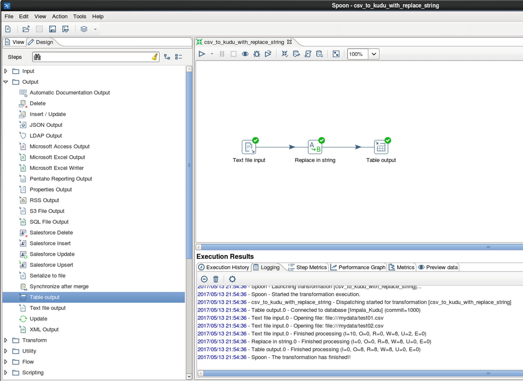
Run the job
Check the table and make sure “Yonkers” is replaced with “Berkeley.” Compare the value of the city in row id 5 with the original source text file.
SQL Server to Kudu
In this example, we’ll show how to ingest data from an RDBMS (SQL Server 2016) to Kudu.
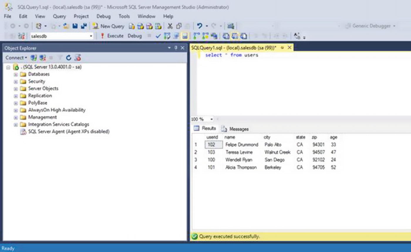
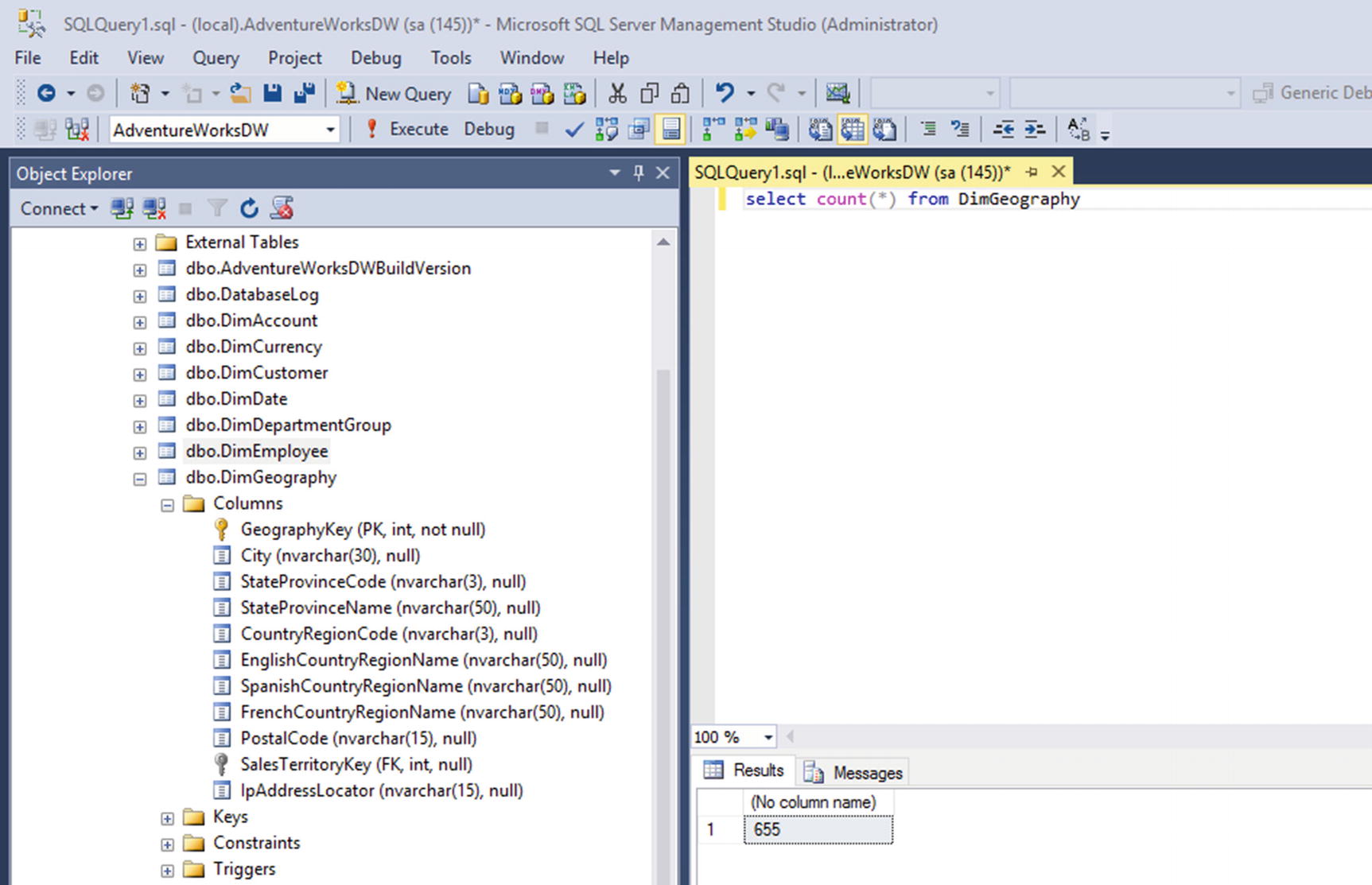
Check the table in SQL Server Management Studio
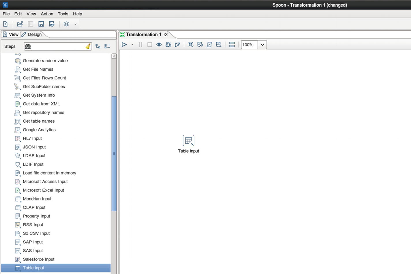
Table input
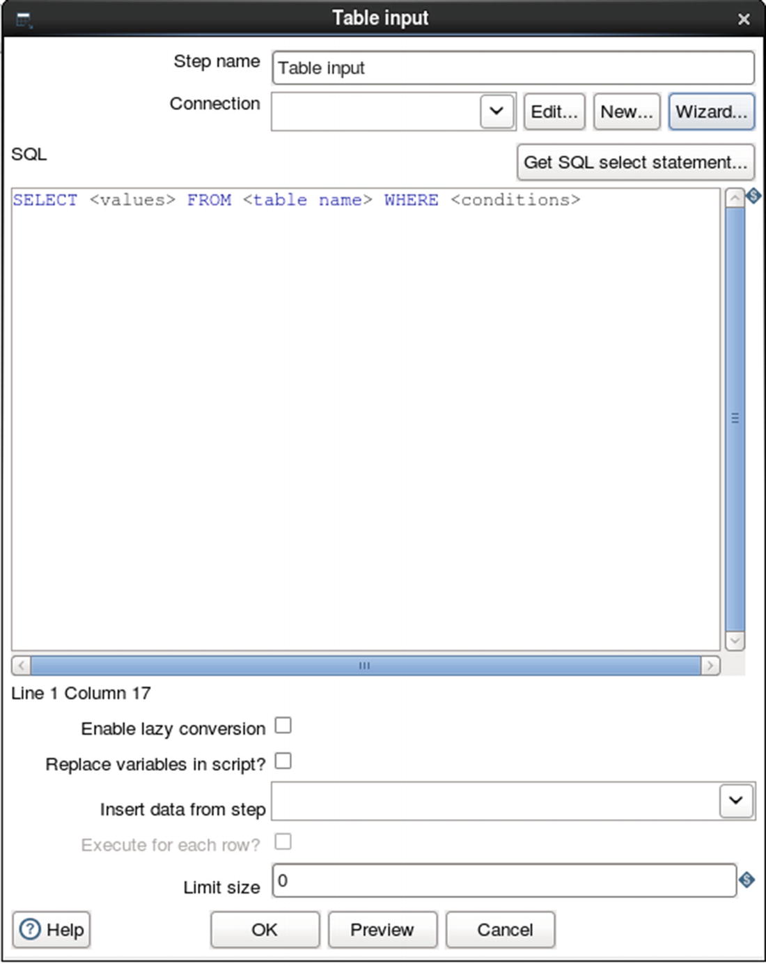
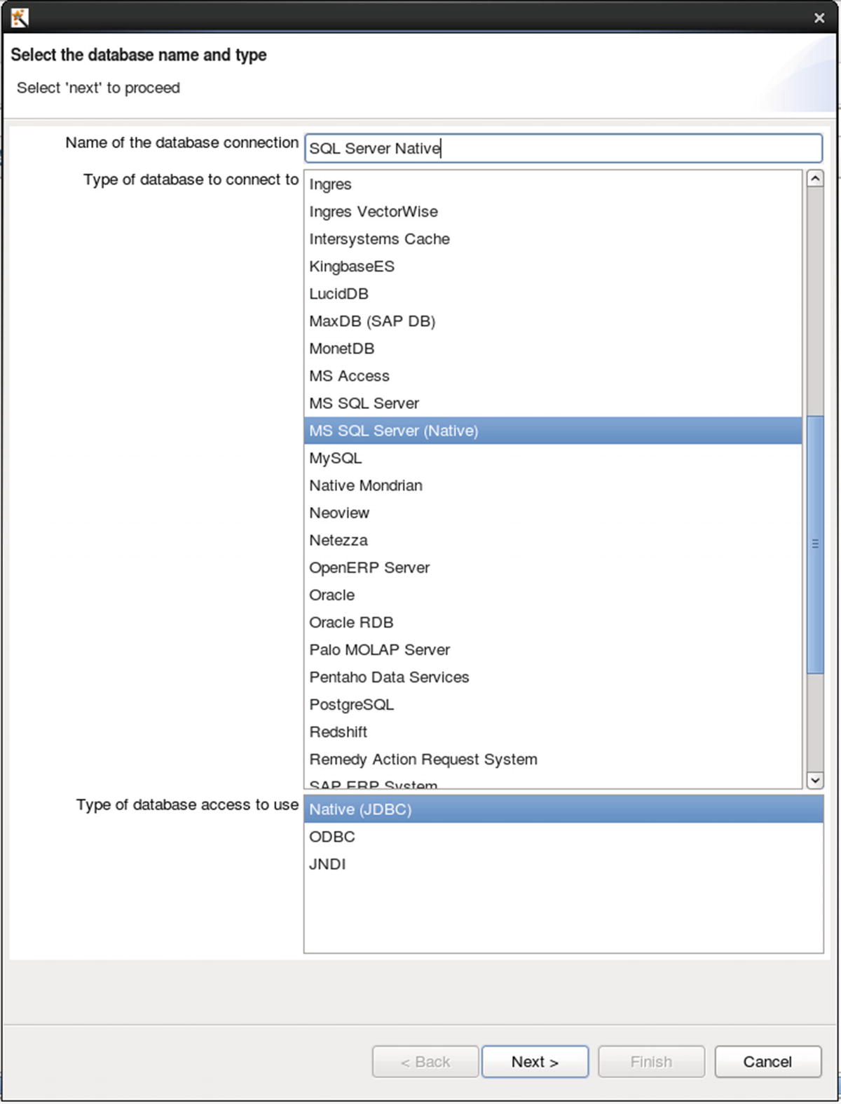
Configure database connection
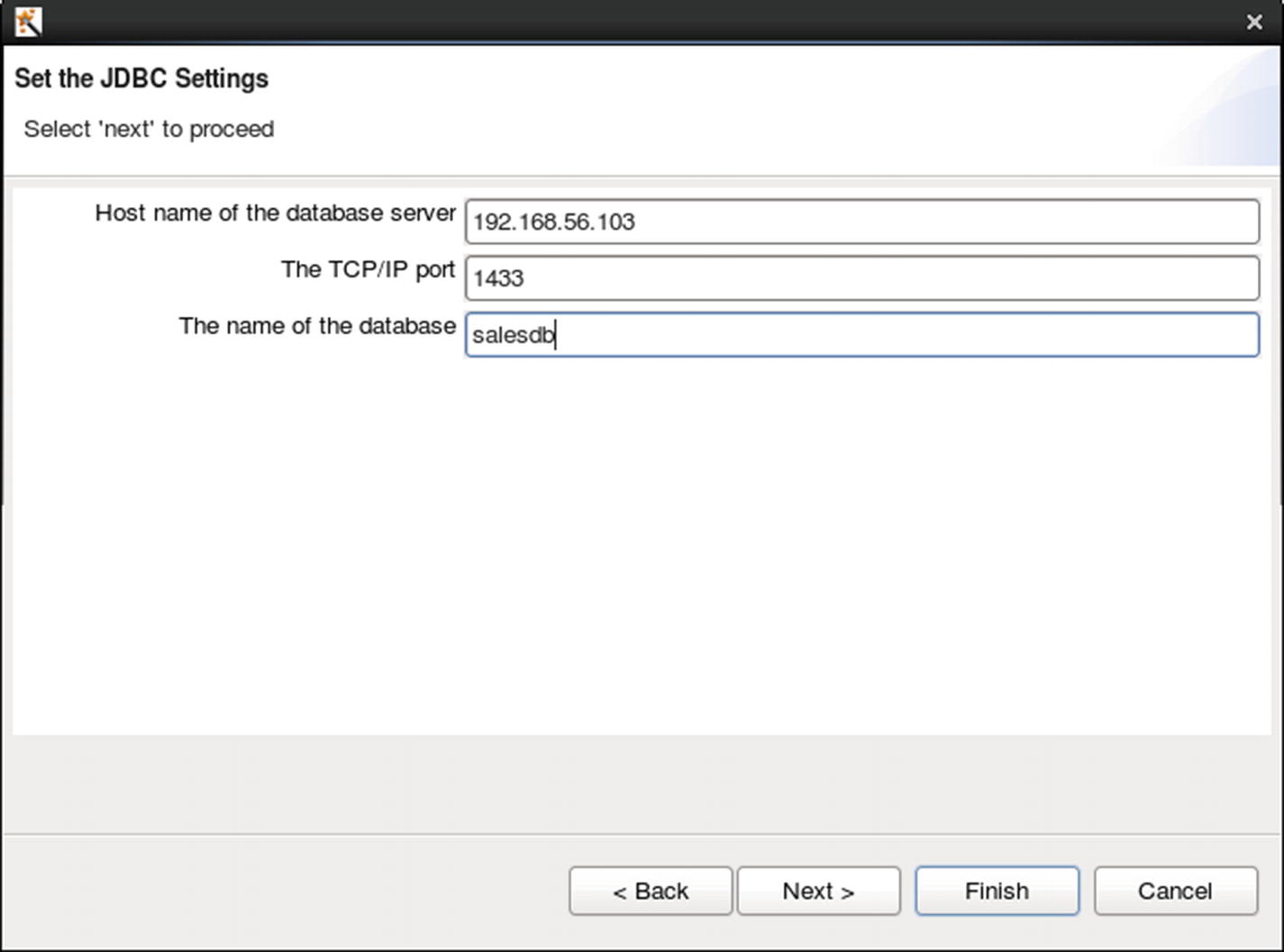
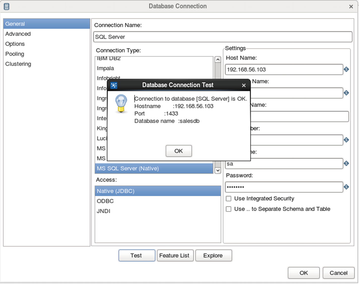
Test database connection
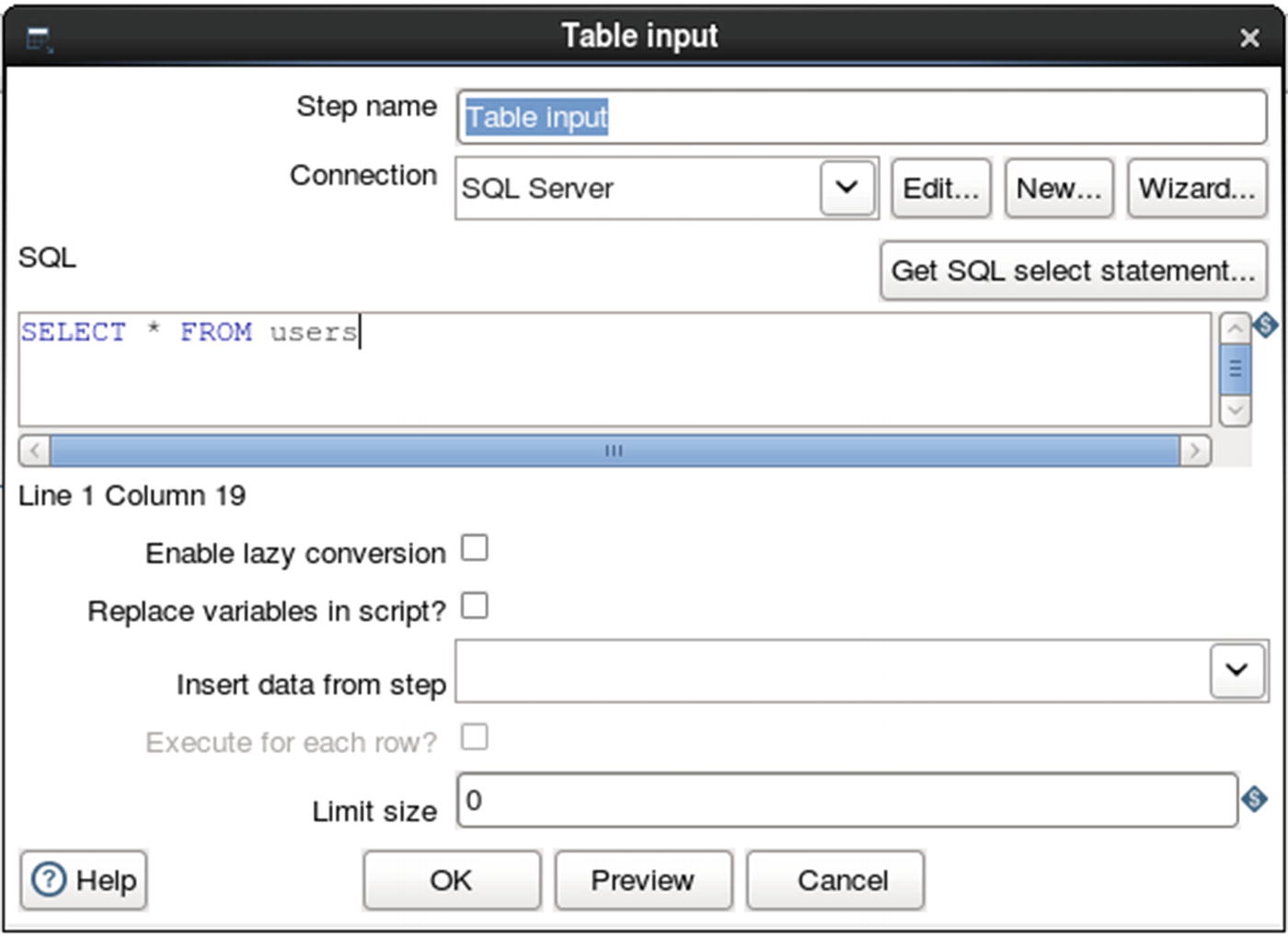
Specify SQL query as data source
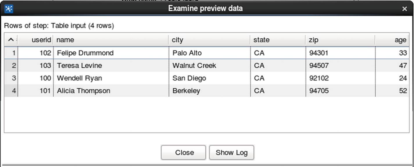
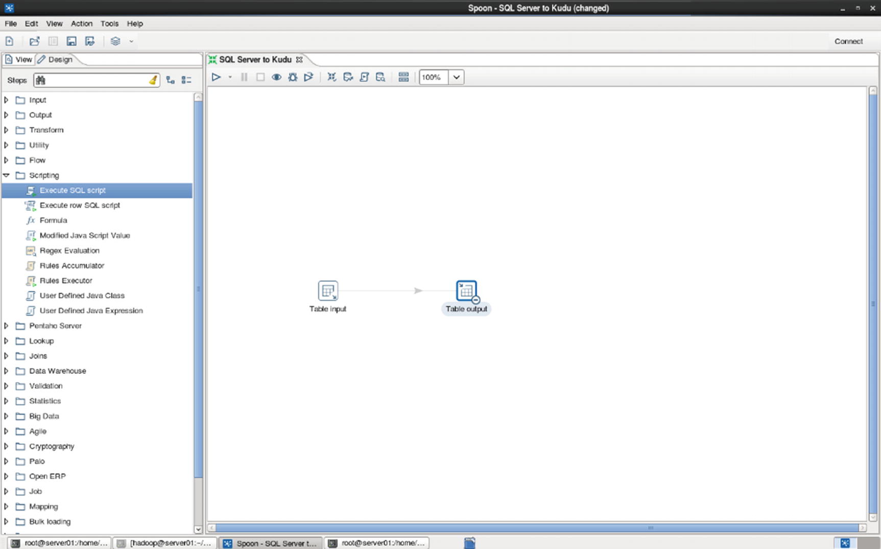
Table output
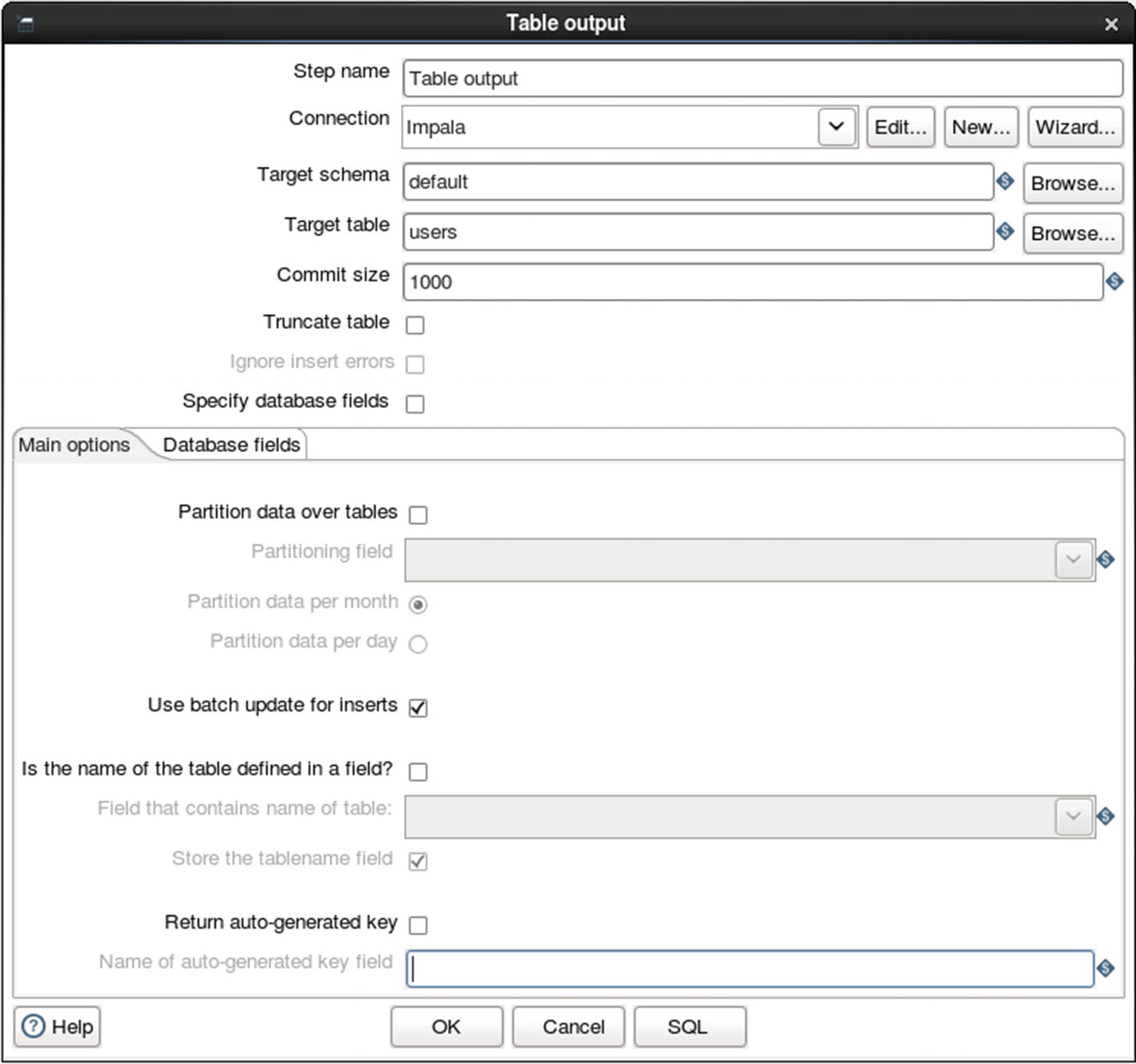
Configure Table output
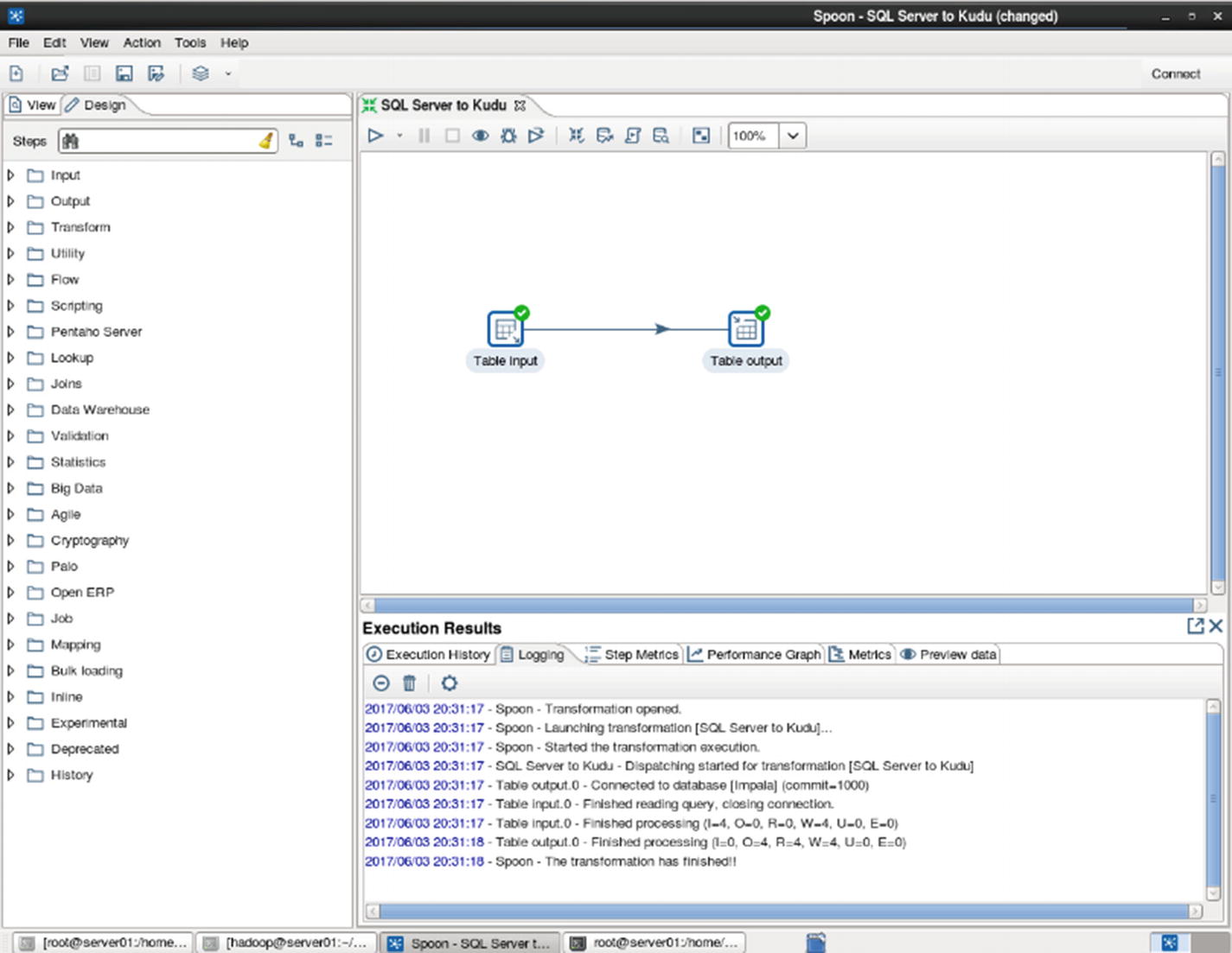
Inspect the logs for errors.
Confirm that the data was successfully inserted to the Kudu table.
Congratulations! You’ve successfully ingested data from SQL Server 2016 to Kudu.
Talend Open Studio
Talend is one of the leading software companies that specializes in big data integration. Talend offers free open source data ingestion tools called Open Studio for Big Data and Open Studio for Data Integration. Both tools provide modern graphical user interface, YARN support, HDFS, HBase, Hive and Kudu support, connectors to Oracle, SQL Server and Teradata, and fully open source under Apache License v2. xx The main difference between Open Studio for Data Integration and Open Studio for Big Data is that Data Integration can only generate native Java code, while Big Data can generate both native Java, Spark and MapReduce code.
The commercial version gives you access to live Talend support, guaranteed response times, upgrades, and product patches. The open source version only provides community support. xxi If you are processing terabytes or petabytes of data, I suggest you use the Big Data edition. For traditional ETL-type workloads such as moving data from an RDBMS to Kudu, with some light data transformation in between, the Data Integration edition is sufficient. We will use Talend Open Studio for Data Integration in this chapter.
Note
Talend Kudu components are provided by a third-party company, One point Ltd. These components are free and downloadable from the Talend Exchange – https://exchange.talend.com/ . The Kudu Output and Input components need to be installed before you can use Talend with Kudu.
Ingesting CSV Files to Kudu
Let’s start with a familiar example of ingesting CSV files to Kudu.
Prepare the test data.
Create the destination Kudu table in Impala.
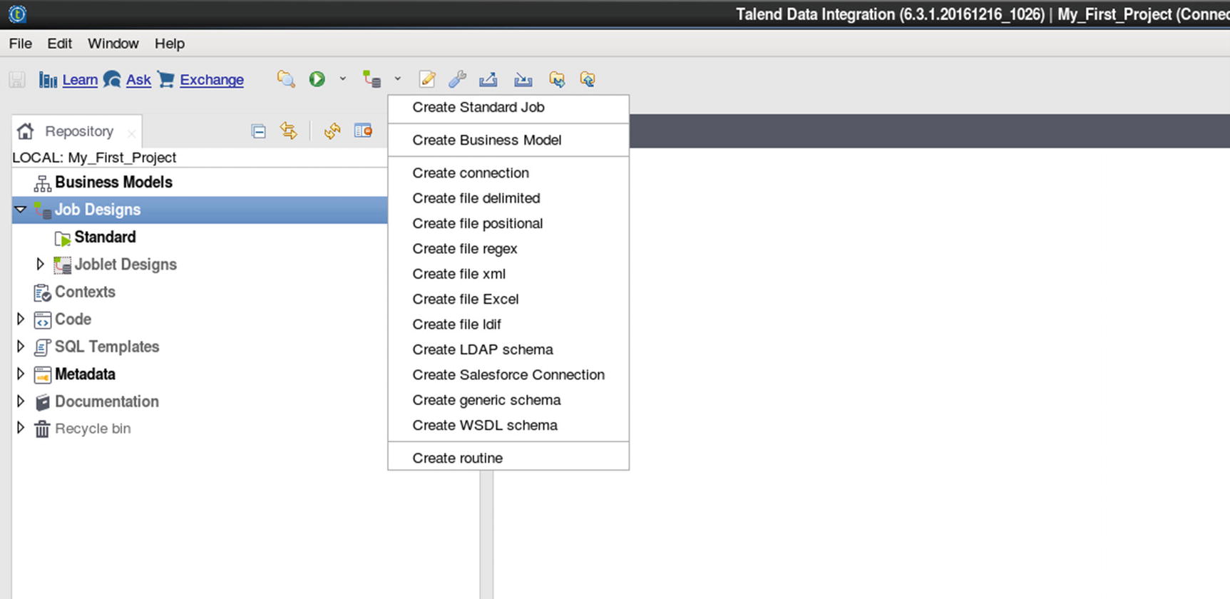
Start Talend Open Studio for Data Integration
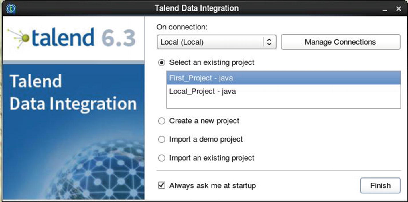
Select an existing project or create a new project
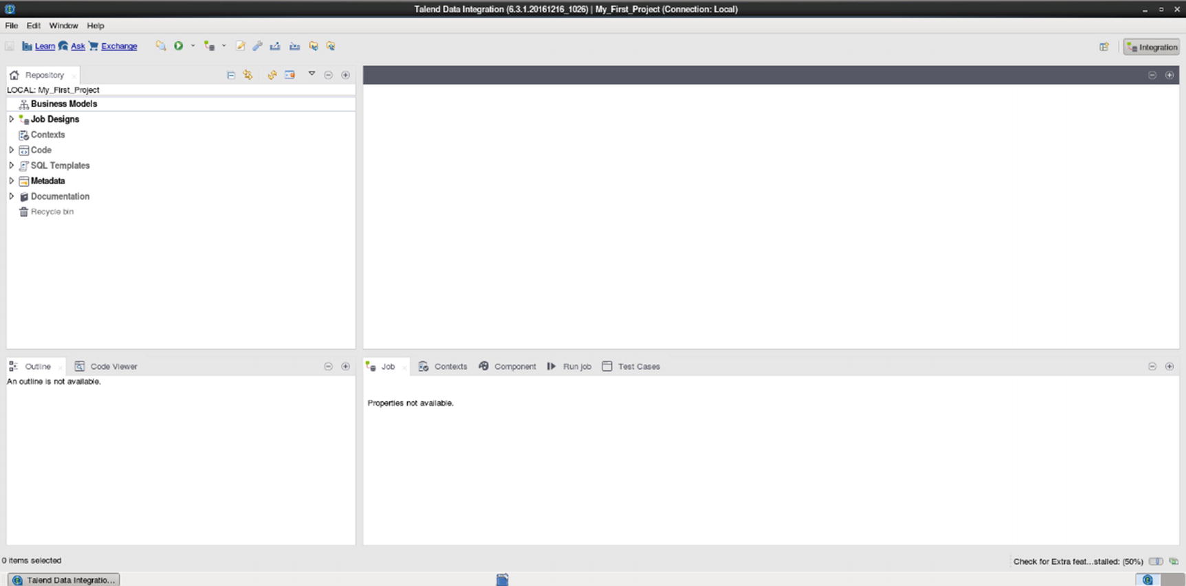
Talend Open Studio Graphical User Interface
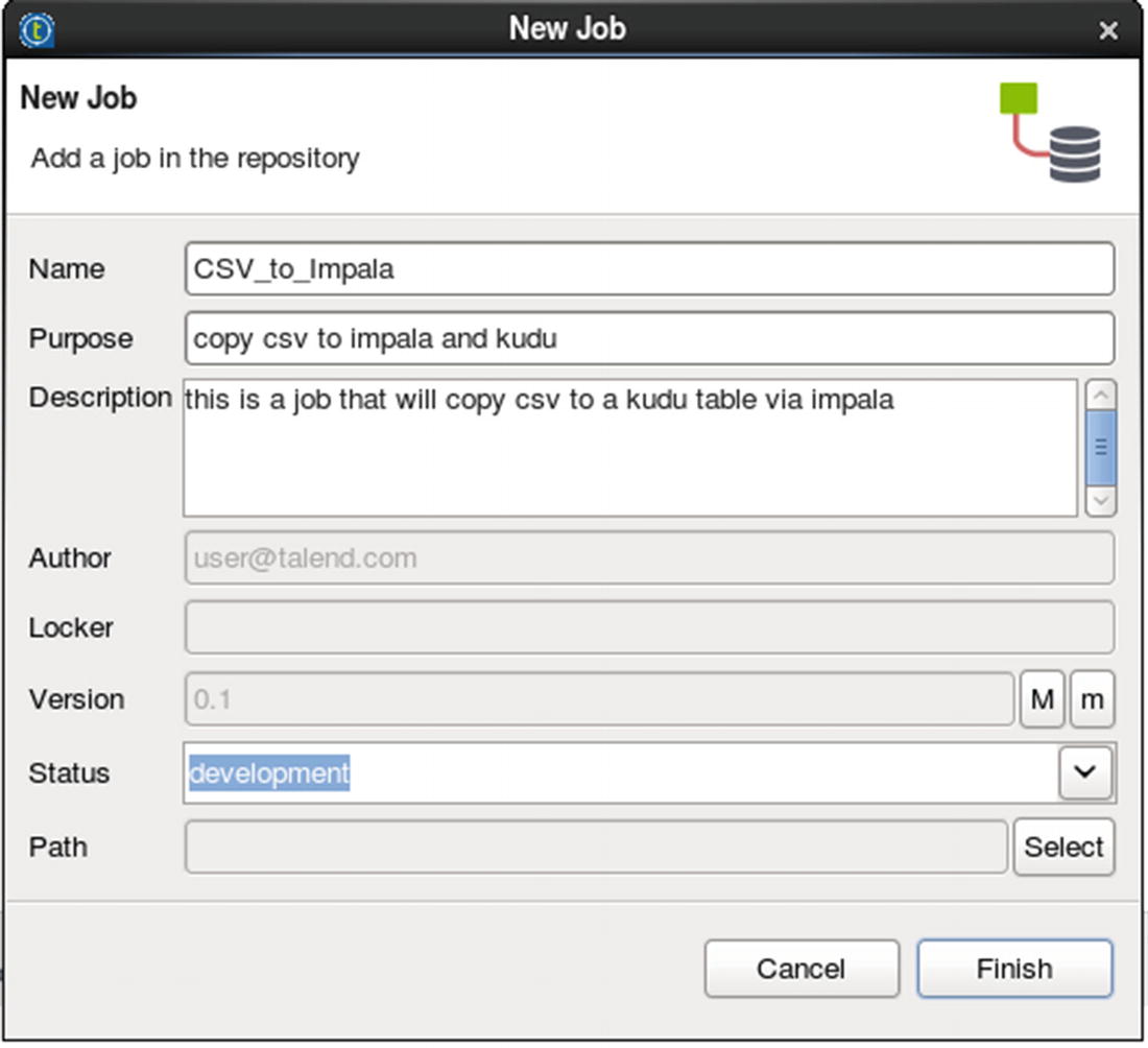
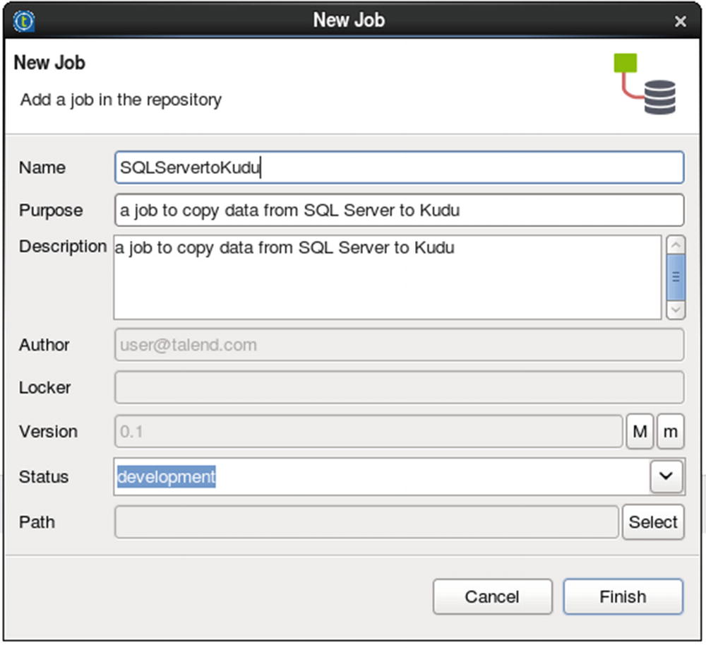
Specify job name and other job properties
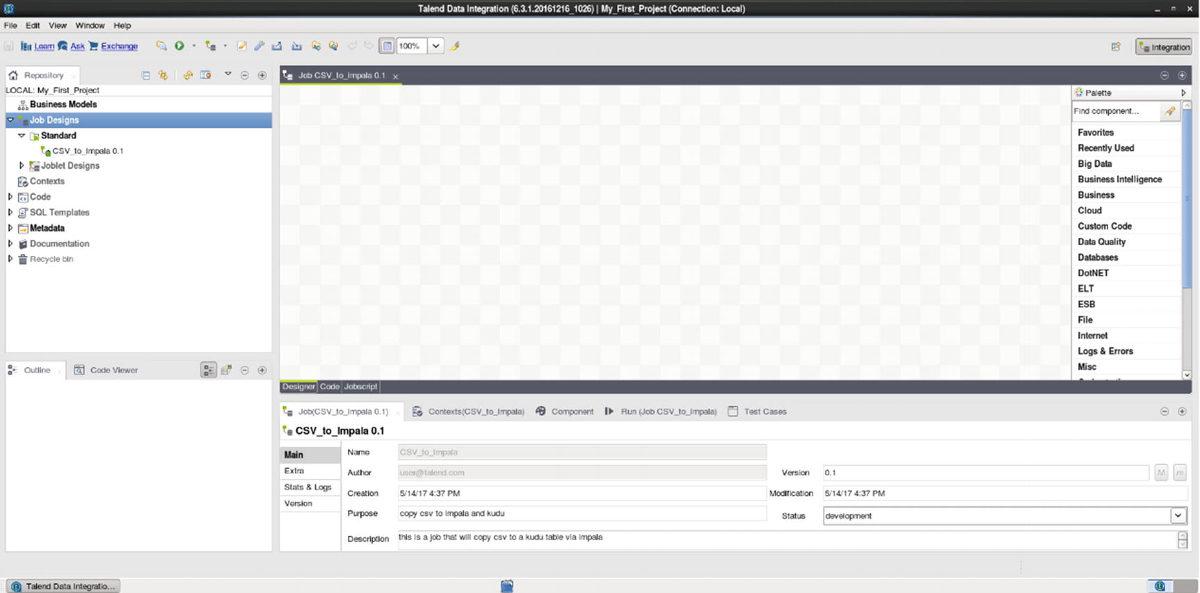
Job canvas
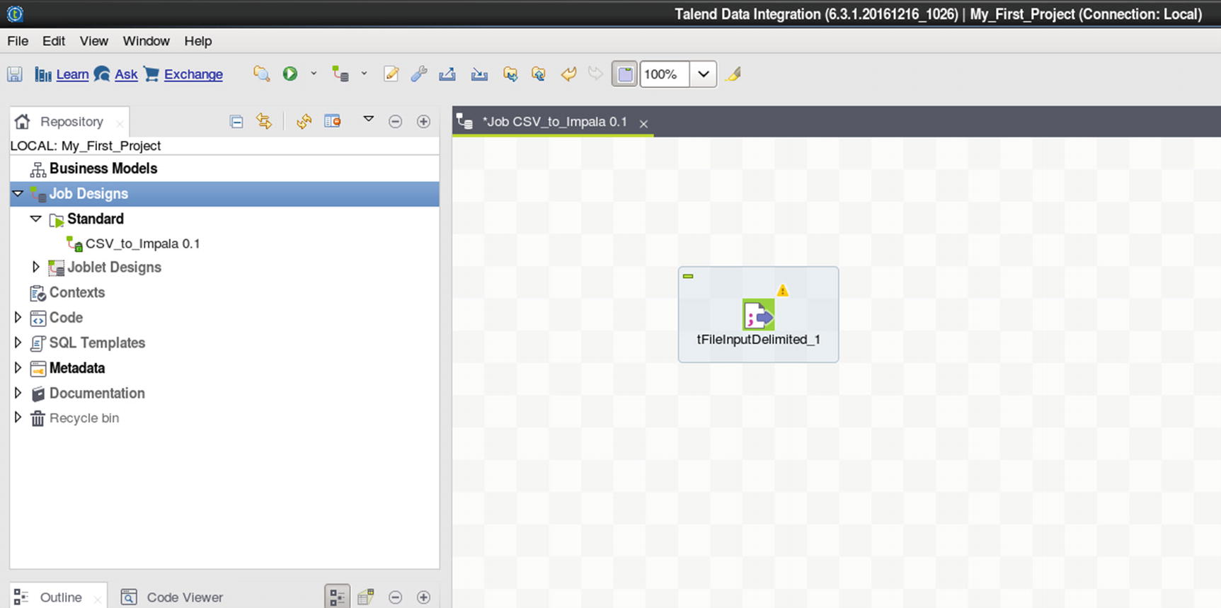
tFileInputDelimited source
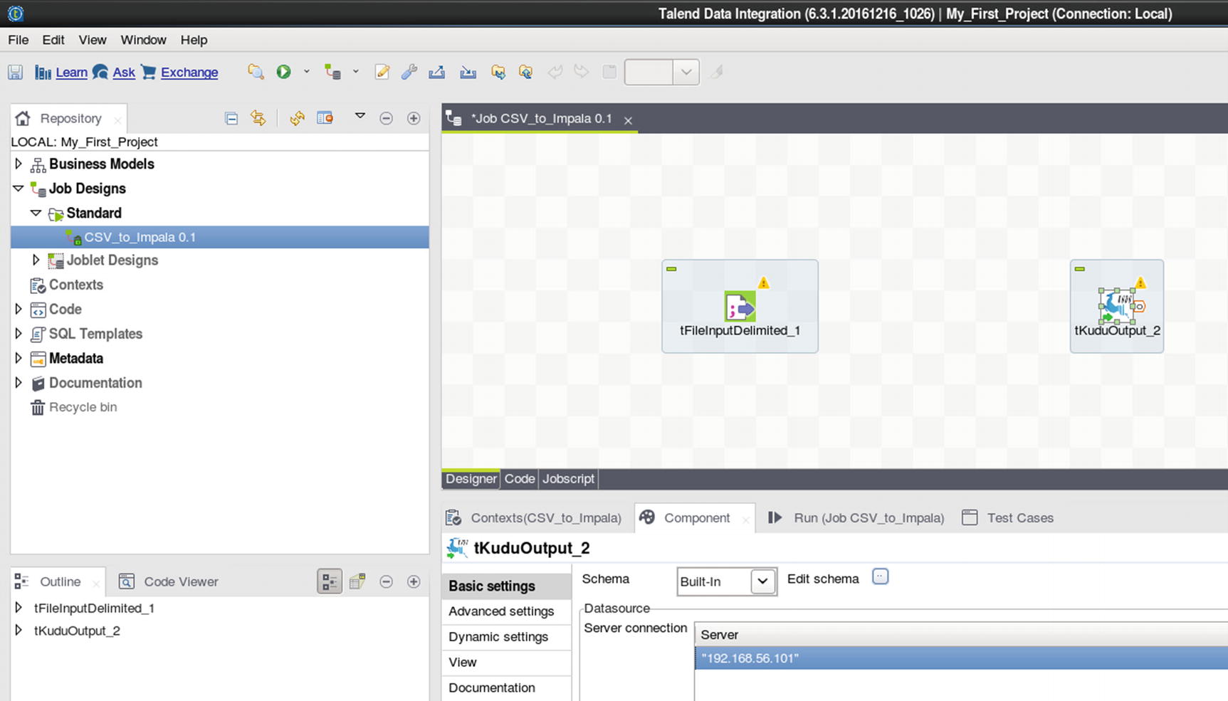
Kudu output
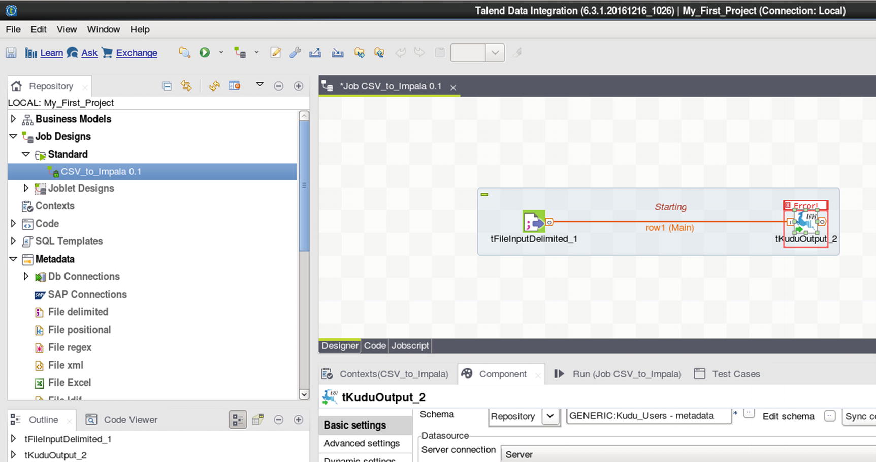
Connect File Input delimited and Kudu output
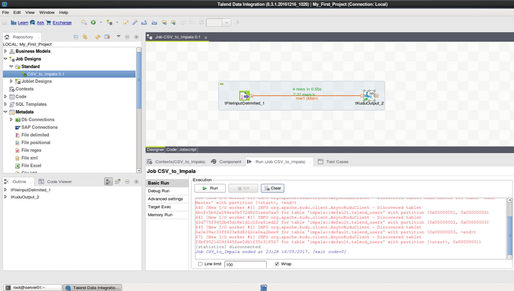
Run the job
The logs will show information about the job while it’s running. You’ll see an exit code when the job completes. An exit code of zero indicates that the job successfully completed.
Confirm that the rows were successfully inserted into the Kudu table.
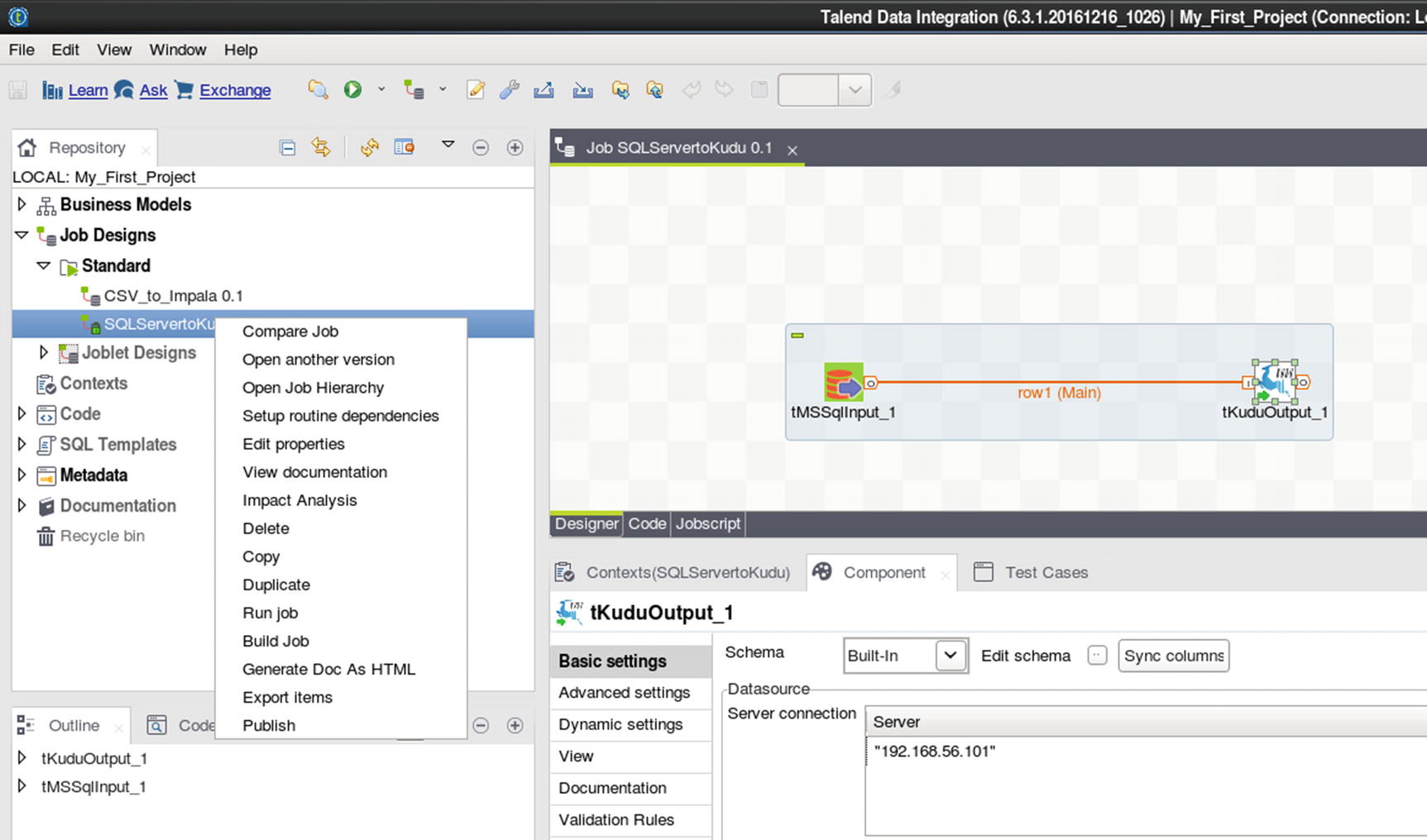
SQL Server to Kudu
For our second example, let’s ingest data from SQL Server to Kudu using Talend Open Studio. Create the Kudu table DimGeography in Impala if you haven’t done it already.
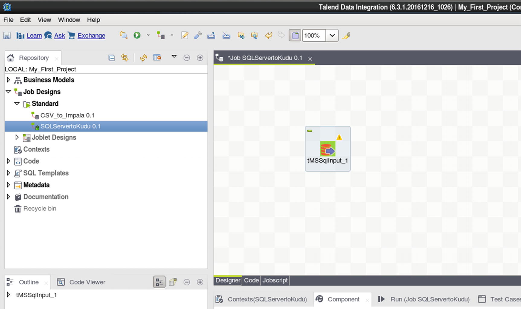
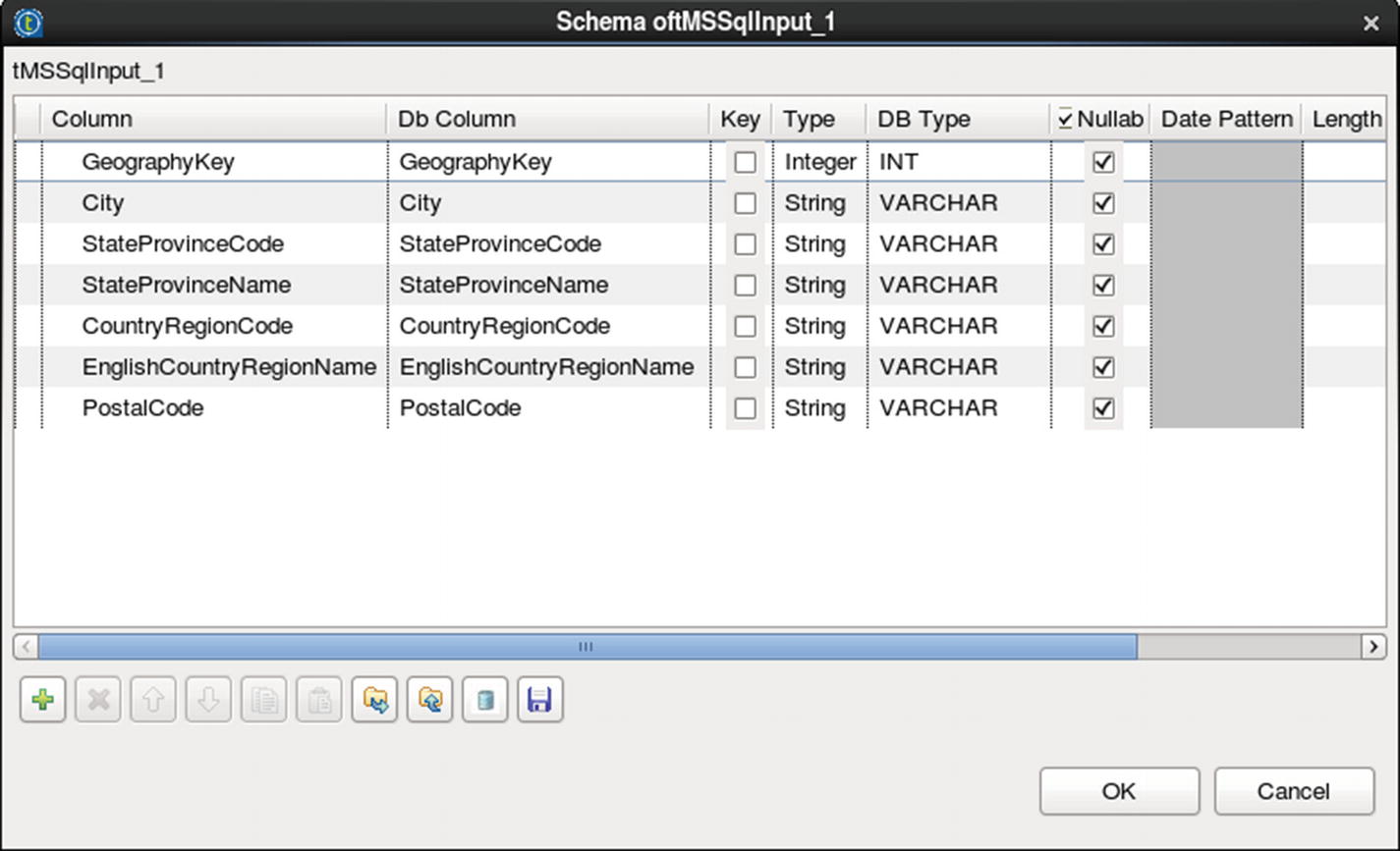
Configure MS SQL input
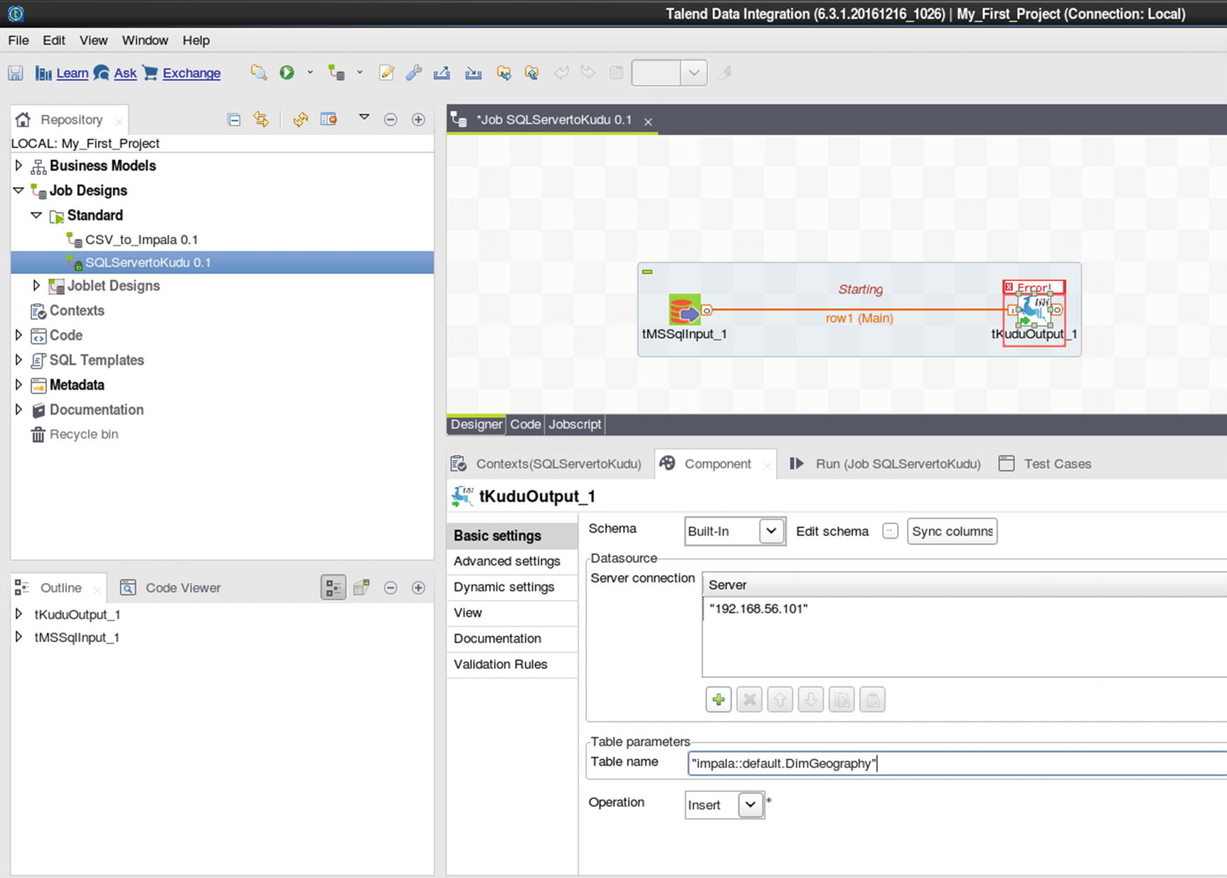
Kudu output
Configure Kudu output
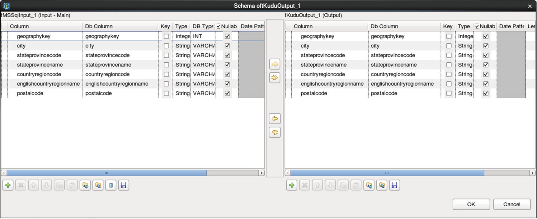
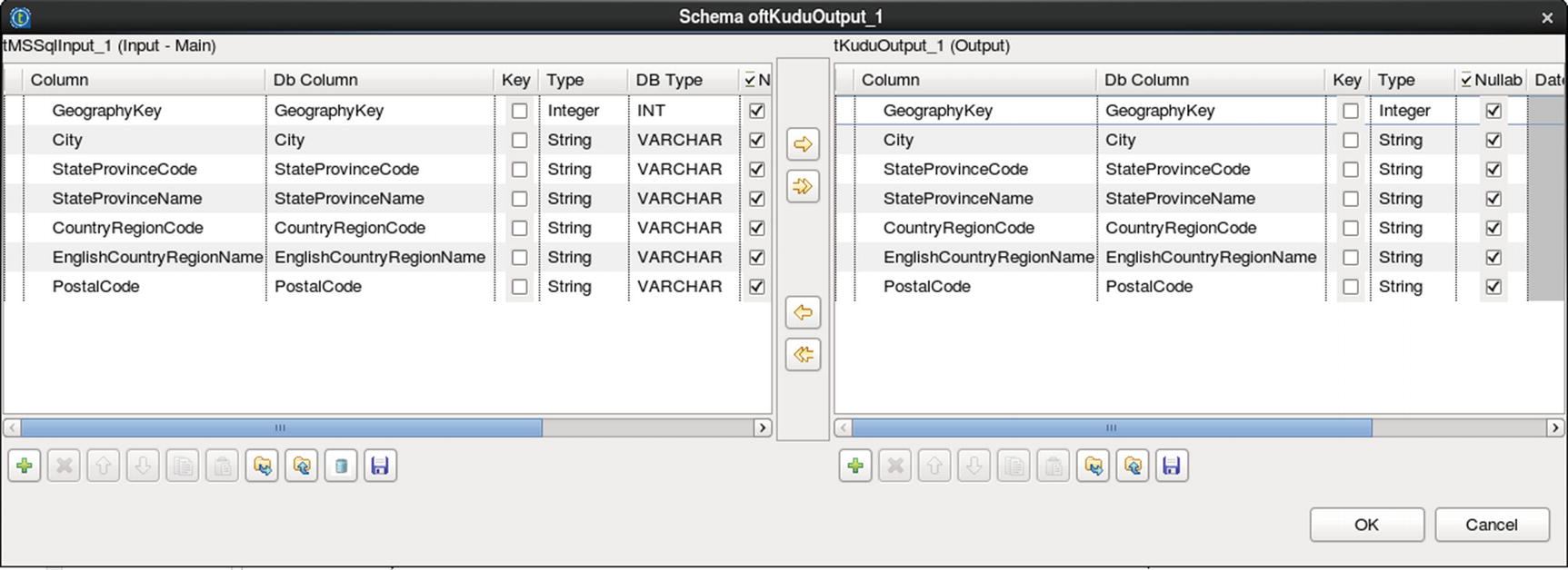
Sync the schema
Run the job
Verify if the job ran successfully
Data Transformation
Let’s now use some of Talend’s built-in features for data transformation. I’ll use the tReplace component to replace a value in the specified input column. We’ll replace the value “United Kingdom” with “UK.” I’ll also use the tFilterRow component to filter results to only include records where city is equal to “London” or “Berkshire.”
Drag and drop the tReplace and tFilterRow components into the canvas, in between the input and the output as shown in Figure 7-136.
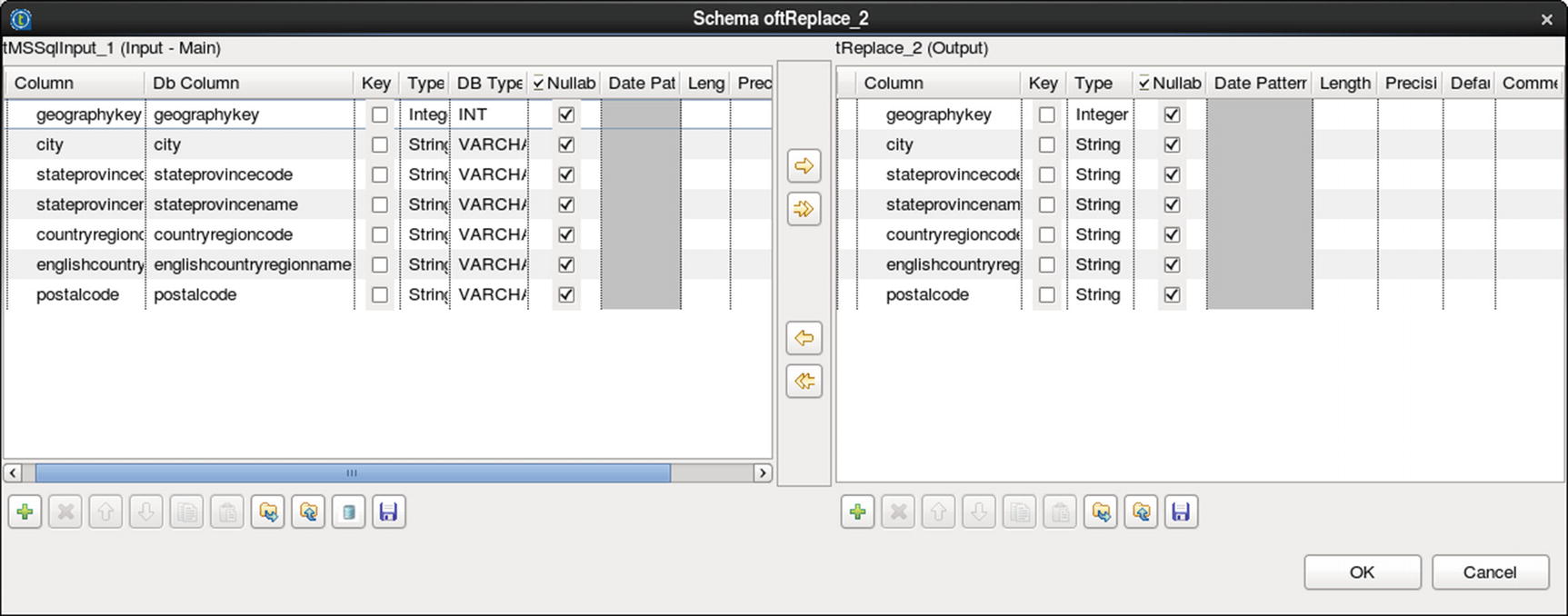
Select field
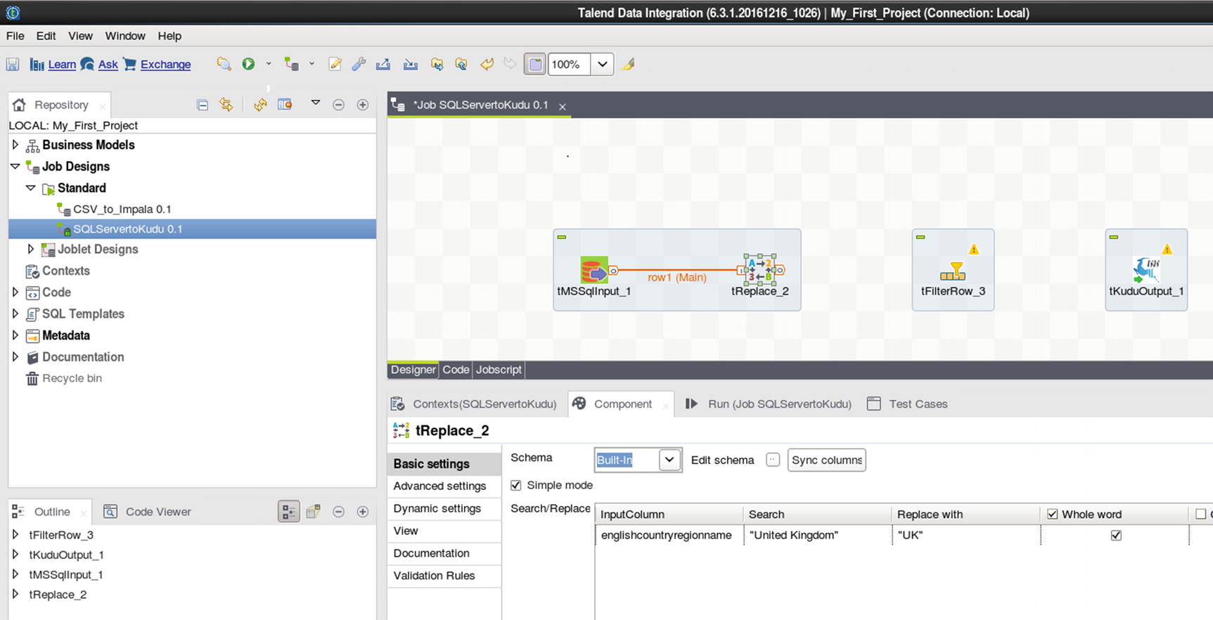
Configure tReplace
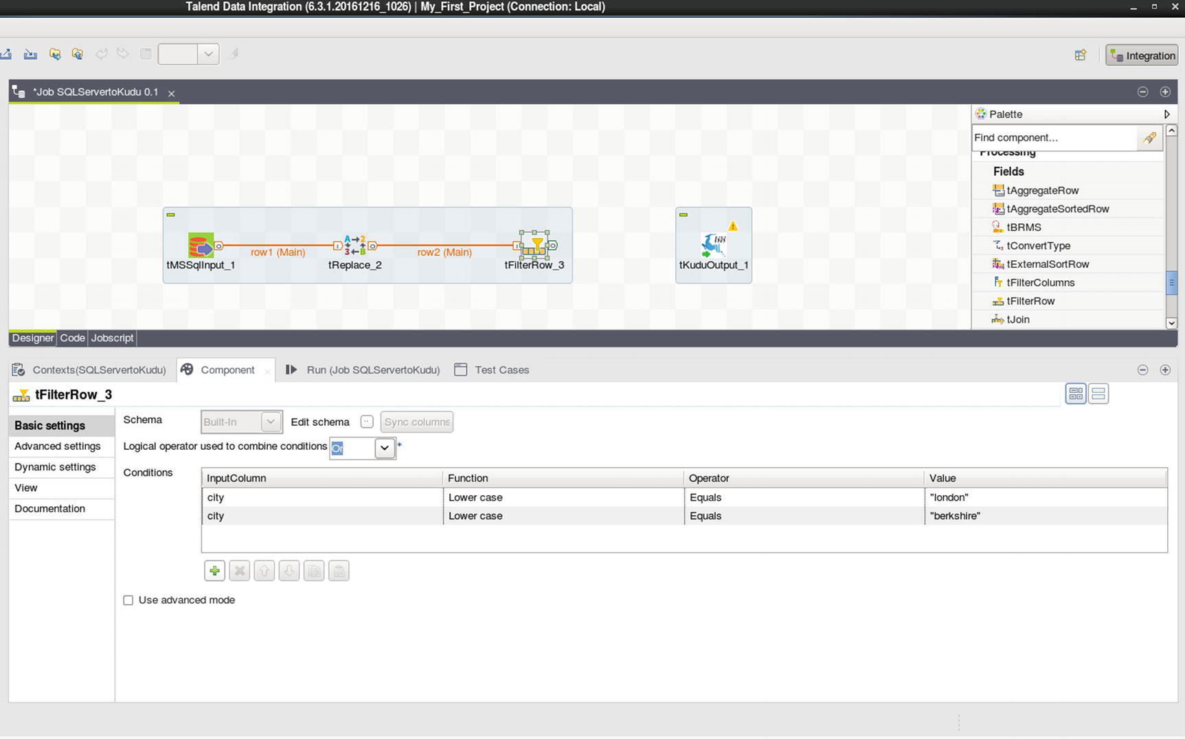
Configure tFilterRow
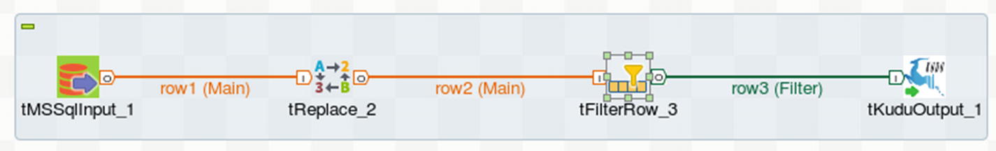
Connect tFilterRow to Kudu output
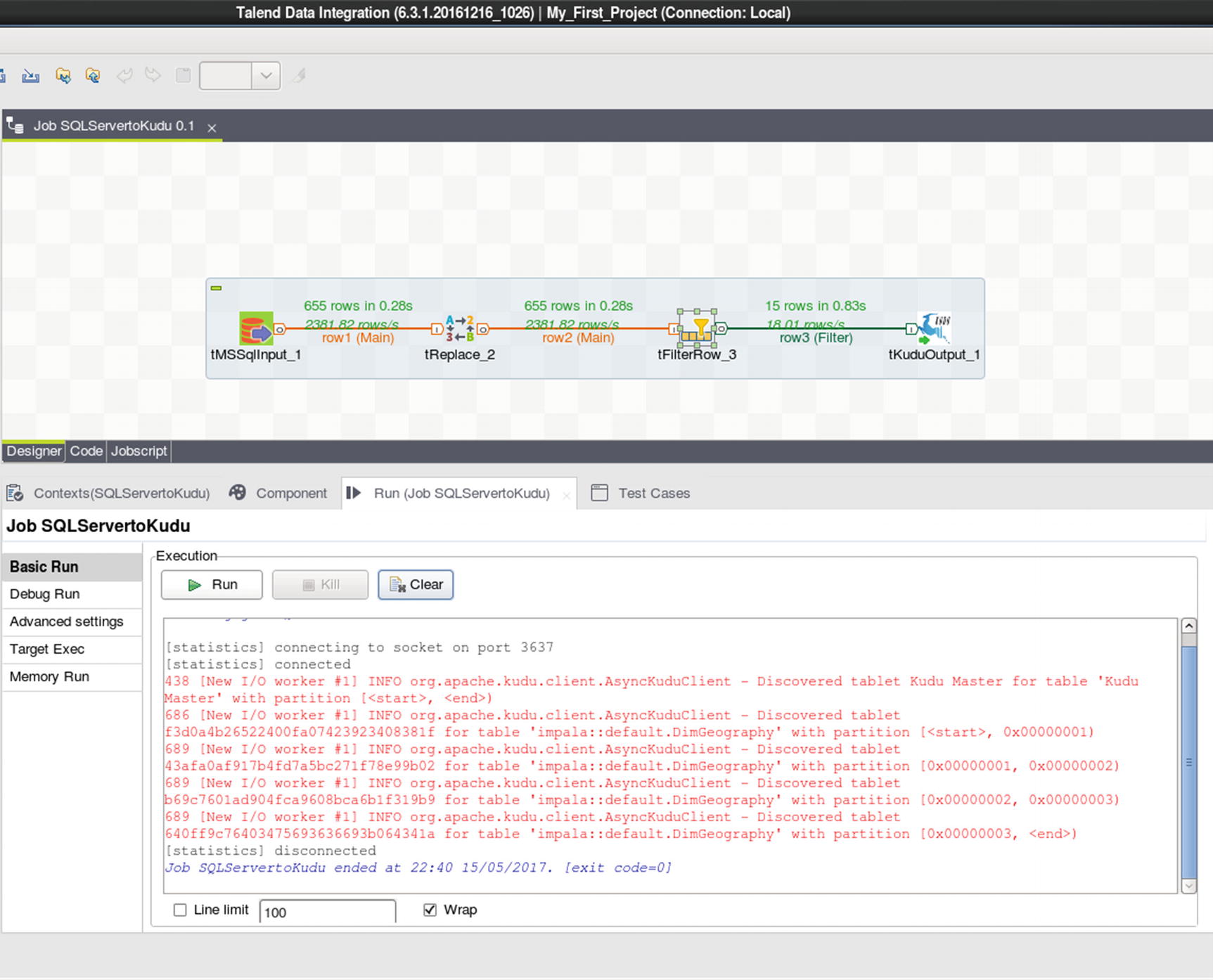
Run the job
Inspect the data in the Kudu table to ensure that the job successfully executed. As you can see from the results, only records where city is equal to London and Berkshire were returned. United Kingdom was also replaced with UK.
Other Big Data Integration Players
This chapter would not be complete if I didn’t mention the traditional ETL players. They’re tools that have been enhanced to include big data integration. Even so, they still lag in terms of native features compared to the newer big data integration tools I just discussed. Most lack native Spark support and connectors to popular big data sources, for example.
Informatica
Informatica is the largest software development company in the world that specializes in data integration. Founded in 1993, the company is based in Redwood City, California. Informatica also develops software for master data management, data quality, b2b data exchange, data virtualization, and more. xxii Informatica PowerCenter Big Data Edition is the company’s flagship product for big data integration. Like the other ETL tools described in this chapter, Informatica PowerCenter Big Data Edition features an easy-to-use visual development environment. Informatica PowerCenter Big Data Edition has tight integration with the leading traditional and big data platforms making it easy for you schedule, manage and monitor processes, and workflows across your enterprise. xxiii As of this writing, Informatica PowerCenter doesn’t have native Kudu support; however you may be able to ingest data into Kudu using Informatica PowerCenter via Impala and JDBC/ODBC.
Microsoft SQL Server Integration Services
This list would not be complete if I didn’t mention the top three largest enterprise software development companies, Microsoft, IBM, and Oracle. SQL Server Integration Services (SSIS) includes features that supports Hadoop and HDFS data integration. SSIS provides the Hadoop Connection Manager and the following Control Flow Tasks: Hadoop File System Task, Hadoop Hive Task, and Hadoop Pig Task. SSIS supports the following data source and destination: HDFS File Source and HDFS File Destination. As with all the ETL tools described in this chapter, SSIS also sports a GUI development environment. xxiv As of this writing, SSIS doesn’t have native Kudu support; however you may be able to ingest data into Kudu via Impala and JDBC/ODBC.
Oracle Data Integrator for Big Data
Oracle Data Integrator for Big Data provides advanced data integration capabilities for big data platforms. It supports a diverse set of workloads, including Spark, Spark Streaming, and Pig transformations and connects to various big data sources such as Kafka and Cassandra. For Orchestration of ODI jobs, users have a choice between using ODI agents or Oozie as orchestration engines. xxv As of this writing, Oracle Data Integrator doesn’t have native Kudu support; however you may be able to ingest data into Kudu using Oracle Data Integrator via Impala and JDBC/ODBC.
IBM InfoSphere DataStage
IBM InfoSphere DataStage is IBM’s data integration tool that comes with IBM InfoSphere Information Server. It supports extract, transform, and load (ETL) and extract, load, and transform (ELT) patterns. xxvi It provides some big data support such as accessing and processing files on HDFS and moving tables from Hive to an RDBMS. xxvii The IBM InfoSphere Information Server operations console can be used to monitor and administer DataStage jobs, including monitoring their job logs and resource usage. The operations console also aids in troubleshooting issues when runtime issues occur. xxviii As of this writing, DataStage doesn’t have native Kudu support; however you may be able to ingest data into Kudu using DataStage via Impala and JDBC/ODBC.
Syncsort
Syncsort is another leading software development company specializing in big data integration. They are well known for their extensive support for mainframes. By 2013, Syncsort had positioned itself as a “Big Iron to Big Data” data integration company. xxix
Syncsort DMX-h, Syncsort’s big data integration platform, has a batch and streaming interfaces that can collect different types of data from multiple sources such as Kafka, HBase, RDBMS, S3, and Mainframes. xxx Like the other ETL solutions described in this chapter, Syncsort features an easy-to-use GUI for ETL development. xxxi As of this writing, DMX-h doesn’t have native Kudu support; however you may be able to ingest data into Kudu using DMX-h via Impala and JDBC/ODBC.
Apache NIFI
Apache NIFI is an open source real-time data ingestion tool mostly used in the Hortonworks environment, although it can be used to ingest data to and from other platforms such as Cloudera and MapR. It’s similar to StreamSets in many aspects. One of the main limitations of NIFI is its lack of YARN support. NIFI runs as an independent JVM process or multiple JVM processes if configured in cluster mode. xxxii NIFI does not have native Kudu support at the time of this writing, although the open source community is working on this. Check out NIFI-3973 for more details. xxxiii
Data Ingestion with Native Tools
Ten years ago, you had to be Java developer in order to ingest and process data with Hadoop. Dozens of lines of code were often required to perform simple data ingestion or processing. Today, thanks to the thousands of committers and contributors to various Apache projects, the Hadoop ecosystem has a whole heap of (and some say too many) native tools for data ingestion and processing. Some of these tools can be used to ingest data into Kudu. I’ll show examples using Flume, Kafka, and Spark. If you want to develop your own data ingestion routines, Kudu provides APIs for Spark, Java, C++, and Python.
Kudu and Spark
Kudu provides a Spark API that you can use to ingest data into Kudu tables. In the following example, we’ll join a table stored in a SQL Server database with another table stored in an Oracle database and insert the joined data into a Kudu table. Chapter 6 provides a more thorough discussion of Kudu and Spark.
Start the spark-shell. Don’t forget to include the necessary drivers and dependencies.
Set up the Oracle connection
Create a dataframe from the Oracle table.
Register the table so we can run SQL against it.
Set up the SQL Server connection.
Create a dataframe from the SQL Server table.
Register the table so that we can join it to the Oracle table.
Join both tables. We'll insert the results to a Kudu table.
You can also join the dataframes using the following method.
Create the destination Kudu table in Impala.
Go back to the spark-shell and set up the Kudu connection.
Insert the data to Kudu.
Confirm that the data was successfully inserted into the Kudu table.
Flume, Kafka, and Spark Streaming
Using Flume, Kafka, and Spark Streaming for real-time data ingestion and event processing is a common architectural pattern.Apache Flume
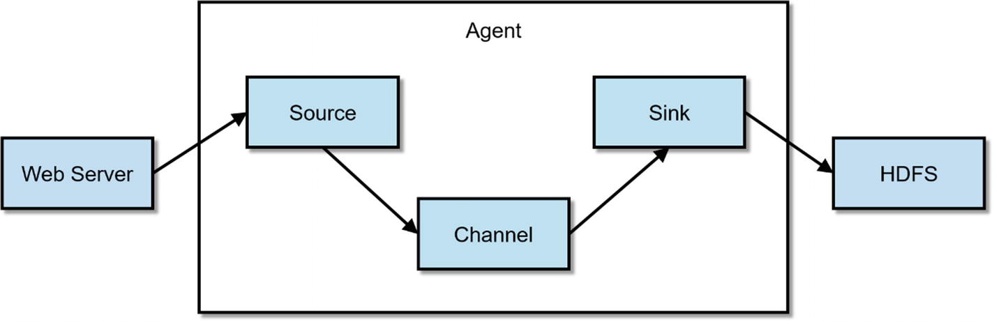
Flume Architecture
Flume is configured using a simple configuration file. The example configuration file lets you generate events from a script and then logs them to the console.
To learn more about Flume, Using Flume (O’Reilly, 2014) by Hari Shreedharan is the definitive guide.
Apache Kafka
Kafka is a fast, scalable, and reliable distributed publish-subscribe messaging system. Kafka is now a standard component of architectures that requires real-time data ingestion and streaming. Although not required, Kafka is frequently used with Apache Flume, Storm, Spark Streaming, and StreamSets.
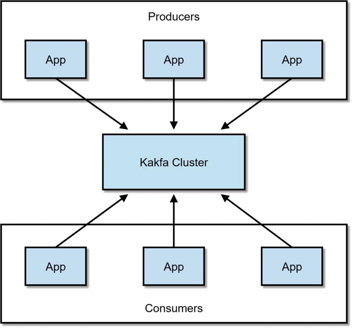
Kafka Producers and Consumers
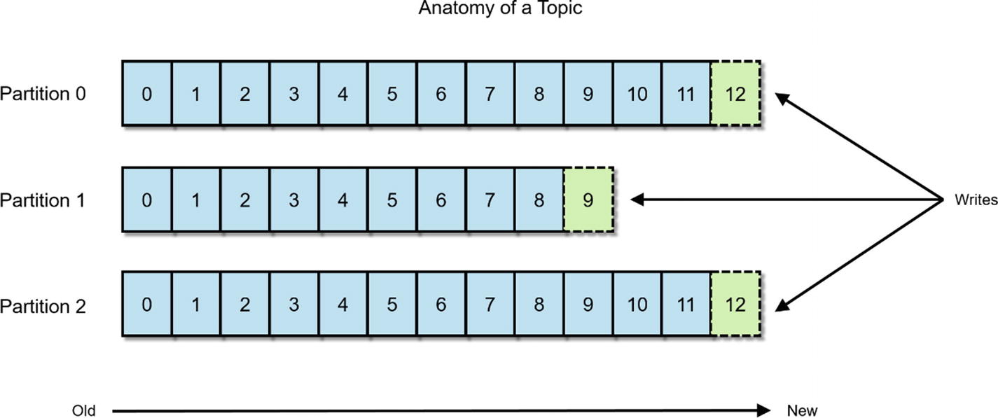
Kafka Topic
To learn more about Kafka, Kafka: The Definitive Guide (O’Reilly, 2017) by Shapiro, Narkhede, and Paling, is the best resource available.
Flafka

A typical Flafka pipeline
The engineers at Cloudera and others in the open source community recognized the benefits of integrating Flume with Kafka, so they developed Flume and Kafka integration frequently referred to as Flafka. Starting in CDH 5.2, Flume can act as consumer and producer for Kafka. With further development included in Flume 1.6 and CDH 5.3, the ability for Kafka to act as a Flume channel has been added. xxxvi
Spark Streaming
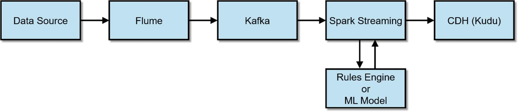
A typical Flafka pipeline with Spark Streaming and Kudu
Sqoop
Sqoop is not technically compatible with Kudu. You cannot use Sqoop to transfer data from an RDBMS to Kudu and vice versa. However, Sqoop may be the only tool some users may have for ingesting data from an RDBMS.
What you can do is to use Sqoop to ingest data from an RDBMS into HDFS and then use Spark or Impala to read the data from HDFS and insert it into Kudu. Here’s a few examples of what you can do with Sqoop. Make sure you install and configure the correct drivers.
Get a list of available databases in SQL Server.
Copy a table from SQL Server to Hadoop.
Copy a table from Hive to SQL Server.
Then you can just simply execute an Impala insert into…select statement:
Kudu Client API
Kudu provides NoSQL-style Java, C++, and Python client APIs. Applications that requires the best performance from Kudu should use the client APIs. In fact, some of the data ingestion tools discussed earlier, such as StreamSets, CDAP, and Talend utilizes the client APIs to ingest data into Kudu. DML changes via the API is available for querying in Impala immediately without the need to execute INVALIDATE METADATA. Refer Chapter 2 for more details on the Kudu client API.
MapReduce and Kudu
If your organization still uses MapReduce , you may be delighted to know that Kudu integrates with MapReduce. Example MapReduce code can be found on Kudu’s official website. xxxvii
Summary
There are several ways to ingest data into Kudu. You can use third-party commercials tools such as StreamSets and Talend. You can create your own applications using native tools such as Apache Spark and Kudu’s client APIs offers. Kudu enables users to ingest data by batch or real time while running analytic queries at the same time, making it the ideal platform for IoT and advanced analytics. Now that you’ve ingested data into Kudu, you need to extract value out of them. In Chapters 8 and 9, I will discuss common ways to analyze data stored in your Kudu tables.
References
- i.
Business Wire; “StreamSets Raises $12.5 Million in Series A Funding Led by Battery Ventures and NEA,” Business Wire, 2015, https://www.businesswire.com/news/home/20150924005143/en/StreamSets-Raises-12.5-Million-Series-Funding-Led
- ii.
StreamSets; “Conquer Dataflow Chaos,” StreamSets, 2018, https://streamsets.com/
- iii.
Apache Kudu; “Example Use Cases,” Apache Kudu, 2018, https://kudu.apache.org/docs/#kudu_use_cases
- iv.
Tom White; “The Small Files Problem,” Cloudera, 2009, https://blog.cloudera.com/blog/2009/02/the-small-files-problem/
- v.
Aaron Fabri; “Introducing S3Guard: S3 Consistency for Apache Hadoop,” Cloudera, 2017, http://blog.cloudera.com/blog/2017/08/introducing-s3guard-s3-consistency-for-apache-hadoop/
- vi.
Eelco Dolstra; “S3BinaryCacheStore is eventually consistent,” Github, 2017, https://github.com/NixOS/nix/issues/1420
- vii.
Sumologic; “10 Things You Might Not Know About Using S3,” Sumologic, 2018, https://www.sumologic.com/aws/s3/10-things-might-not-know-using-s3/
- viii.
SteamSets; “MQTT Subscriber,” StreamSets, 2018, https://streamsets.com/documentation/datacollector/latest/help/index.html#Origins/MQTTSubscriber.html#concept_ukz_3vt_lz
- ix.
StreamSets; “CoAP Client,” StreamSets, 2018, https://streamsets.com/documentation/datacollector/latest/help/index.html#Destinations/CoAPClient.html#concept_hw5_s3n_sz
- x.
StreamSets; “Read Order,” StreamSets, 2018, https://streamsets.com/documentation/datacollector/latest/help/#datacollector/UserGuide/Origins/Directory.html#concept_qcq_54n_jq
- xi.
StreamSets; “Processing XML Data with Custom Delimiters,” StreamSets, 2018, https://streamsets.com/documentation/datacollector/latest/help/#Pipeline_Design/TextCDelim.html#concept_okt_kmg_jx
- xii.
StreamSets; “Processing XML Data with Custom Delimiters,” StreamSets, 2018, https://streamsets.com/documentation/datacollector/latest/help/#Pipeline_Design/TextCDelim.html#concept_okt_kmg_jx
- xiii.
Arvind Prabhakar; “Tame unruly big data flows with StreamSets,” InfoWorld, 2016, http://www.infoworld.com/article/3138005/analytics/tame-unruly-big-data-flows-with-streamsets.html
- xiv.
StreamSets; “Stream Selector,” StreamSets, 2018, https://streamsets.com/documentation/datacollector/latest/help/#Processors/StreamSelector.html#concept_tqv_t5r_wq
- xv.
StreamSets; “Expression,” StreamSets, 2018, https://streamsets.com/documentation/datacollector/latest/help/#Processors/Expression.html#concept_zm2_pp3_wq
- xvi.
StreamSets; “JavaScript Evaluator,” StreamSets, 2018, https://streamsets.com/documentation/datacollector/latest/help/index.html#Processors/JavaScript.html#concept_n2p_jgf_lr
- xvii.
JSFiddle; “generateUUID,” JSFiddle, 2018, https://jsfiddle.net/briguy37/2MVFd/
- xviii.
Pat Patterson; “Retrieving Metrics via the StreamSets Data Collector REST API,” StreamSets, 2016, https://streamsets.com/blog/retrieving-metrics-via-streamsets-data-collector-rest-api/
- xix.
Pentaho; “Product Comparison,” Pentaho, 2017, https://support.pentaho.com/hc/en-us/articles/205788659-PENTAHO-COMMUNITY-COMMERCIAL-PRODUCT-COMPARISON
- xx.
Talend; “Open Source Integration Software,” Talend, 2018, https://www.talend.com/download/talend-open-studio/
- xxi.
Talend; “Why Upgrade?,” Talend, 2018, https://www.talend.com/products/why-upgrade/
- xxii.
Crunchbase; “Informatica,” Crunchbase, 2018, https://www.crunchbase.com/organization/informatica#/entity
- xxiii.
Informatica; "Informatica PowerCenter Big Data Edition,” Informatica, 2018, https://www.informatica.com/content/dam/informatica-com/global/amer/us/collateral/data-sheet/powercenter-big-data-edition_data-sheet_2194.pdf
- xxiv.
Viral Kothari; “Microsoft SSIS WITH Cloudera BIGDATA,” YouTube, 2016, https://www.youtube.com/watch?v=gPLfcL2zDX8
- xxv.
Oracle; “Oracle Data Integrator For Big Data,” Oracle, 2018, http://www.oracle.com/us/products/middleware/data-integration/odieebd-ds-2464372.pdf ;
- xxvi.
IBM; “Overview of InfoSphere DataStage,” IBM, 2018, https://www.ibm.com/support/knowledgecenter/SSZJPZ_11.5.0/com.ibm.swg.im.iis.ds.intro.doc/topics/what_is_ds.html
- xxvii.
IBM; “Big data processing,” IBM, 2018, https://www.ibm.com/support/knowledgecenter/SSZJPZ_11.5.0/com.ibm.swg.im.iis.ds.intro.doc/topics/ds_samples_bigdata.html
- xxviii.
IBM Analytic Skills; “Monitoring DataStage jobs using the IBM InfoSphere Information Server Operations Console,” IBM, 2013, https://www.youtube.com/watch?v=qOl_6HqyVes
- xxix.
SyncSort; “Innovative Software from Big Iron to Big Data,” SyncSort, 2018, http://www.syncsort.com/en/About/Syncsort-History
- xxx.
SyncSort; “Syncsort DMX-h,” SyncSort, 2018, http://www.syncsort.com/en/Products/BigData/DMXh
- xxxi.
SyncSort; “Introduction to Syncsort DMX-h 8,” SyncSort, 2015, https://www.youtube.com/watch?v=7e_8YadLa9E
- xxxii.
Hortonworks; “APACHE NIFI,” Hortonworks, 2018, https://hortonworks.com/apache/nifi/
- xxxiii.
Jira; “Create a new Kudu Processor to ingest data,” Jira, 2017, https://issues.apache.org/jira/browse/NIFI-3973
- xxxiv.
Apache Flume; “Flume 1.8.0 User Guide,” Apache Flume, 2018, https://flume.apache.org/FlumeUserGuide.html
- xxxv.
Apache Kafka; “Introduction,” Apache Kafka, 2018, https://kafka.apache.org/intro
- xxxvi.
Gwen Shapira, Jeff Holoman; “Flafka: Apache Flume Meets Apache Kafka for Event Processing,” Cloudera, 2014, http://blog.cloudera.com/blog/2014/11/flafka-apache-flume-meets-apache-kafka-for-event-processing/
- xxxvii.
Dan Burkert; “ImportCsv.java,” Apache Kudu, 2017, https://github.com/apache/kudu/blob/master/java/kudu-client-tools/src/main/java/org/apache/kudu/mapreduce/tools/ImportCsv.java