
CHAPTER 11: Sorting and Searching Algorithms
Ake13bk/Shutterstock
At many points in this text we have gone to great trouble to keep information in sorted order: famous people sorted by name or year of birth, airline routes sorted by distance, integers sorted from smallest to largest, and words sorted alphabetically. One reason to keep lists sorted is to facilitate searching; given an appropriate implementation structure, a particular list element can be found faster if the list is sorted.
In this chapter we directly examine several strategies for both sorting and searching, contrast and compare them, and discuss sorting/searching concerns in general. Even though sorting and searching are already supported by most modern software development platforms, we believe their study is beneficial for computer science students—for the same reasons you study data structures even though language libraries provide powerful structuring APIs, you should study sorting and searching. Their study provides a good way to learn basic algorithmic and analysis techniques that help form a foundation of problem-solving tools. Studying the fundamentals prepares you for further growth so that eventually you will be able to create your own unique solutions to the unique problems that you are sure to encounter one day.
11.1 Sorting
Putting an unsorted list of data elements into order—sorting—is a very common and useful operation. Entire books have been written about sorting algorithms as well as algorithms for searching a sorted list to find a particular element.
Because sorting a large number of elements can be extremely time consuming, an efficient sorting algorithm is very important. How do we describe efficiency? List element comparison—that is, the operation that compares two list elements to see which is smaller—is an operation central to most sorting algorithms. We use the number of required element comparisons as a measure of the efficiency of each algorithm. For each algorithm we calculate the number of comparisons relative to the size of the list being sorted. We then use order of growth notation, based on the result of our calculation, to succinctly describe the efficiency of the algorithm.
In addition to comparing elements, each of our algorithms includes another basic operation: swapping the locations of two elements on the list. The number of element swaps needed to sort a list is another measure of sorting efficiency. In the exercises we ask you to analyze the sorting algorithms developed in this chapter in terms of that alternative measure.
Another efficiency consideration is the amount of extra memory space required by an algorithm. For most applications memory space is not an important factor when choosing a sorting algorithm. We look at only two sorts in which space would be a consideration. The usual time versus space trade-off applies to sorts—more space often means less time, and vice versa.
A Test Harness
To facilitate our study of sorting we develop a standard test harness, a driver program that we can use to test each of our sorting algorithms. Because we are using this program just to test our implementations and facilitate our study, we keep it simple. It consists of a single class called Sorts. The class defines an array that can hold 50 integers. The array is named values. Several static methods are defined:
initValues. Initializes thevaluesarray with random numbers between 0 and 99; uses theabsmethod (absolute value) from the Java library’sMathclass and thenextIntmethod from theRandomclass.isSorted. Returns abooleanvalue indicating whether thevaluesarray is currently sorted.swap. Swapping data values between two array locations is common in many sorting algorithms—this method swaps the integers betweenvalues[index1]andvalues[index2], whereindex1andindex2are parameters of the method.printValues. Prints the contents of thevaluesarray to theSystem.outstream; the output is arranged evenly in 10 columns.
Here is the code for the test harness:
//---------------------------------------------------------------------------
// Sorts.java               by Dale/Joyce/Weems                    Chapter 11
//
// Test harness used to run sorting algorithms.
//---------------------------------------------------------------------------
package ch11.sorts;

import java.util.*;
import java.text.DecimalFormat;

public class Sorts
{
  static final int SIZE = 50;            // size of array to be sorted
  static int[] values = new int[SIZE];   // values to be sorted

  static void initValues()
  // Initializes the values array with random integers from 0 to 99.
  {
    Random rand = new Random();
    for (int index = 0; index < SIZE; index++)
      values[index] = Math.abs(rand.nextInt()) % 100;
  }

  static public boolean isSorted()

  // Returns true if the array values are sorted and false otherwise.
  {
    for (int index = 0; index < (SIZE - 1); index++)
      if (values[index] > values[index + 1])
        return false;
    return true;
  }

  static public void swap(int index1, int index2)
  // Precondition: index1 and index2 are >= 0 and < SIZE.
  //
  // Swaps the integers at locations index1 and index2 of the values array.
  {
    int temp = values[index1];
    values[index1] = values[index2];
    values[index2] = temp;
  }

  static public void printValues()
  // Prints all the values integers.
  {
    int value;
    DecimalFormat fmt = new DecimalFormat("00");
    System.out.println("The values array is:");
    for (int index = 0; index < SIZE; index++)
    {
      value = values[index];
      if (((index + 1) % 10) == 0)
        System.out.println(fmt.format(value));
      else
        System.out.print(fmt.format(value) + " ");
    }
    System.out.println();
  }

  public static void main(String[] args) throws IOException
  {
    initValues();
    printValues();
    System.out.println("values is sorted: " + isSorted());
    System.out.println();

    swap(0, 1);
    printValues();
    System.out.println("values is sorted: " + isSorted());
    System.out.println();
  }
}
In this version of Sorts the main method initializes the values array, prints the array, prints the value of isSorted, swaps the first two values of the array, and again prints information about the array. The output from this class as currently defined would look something like this:
the values array is:
20 49 07 50 45 69 20 07 88 02
89 87 35 98 23 98 61 03 75 48
25 81 97 79 40 78 47 56 24 07
63 39 52 80 11 63 51 45 25 78
35 62 72 05 98 83 05 14 30 23

values is sorted: false

the values array is:
49 20 07 50 45 69 20 07 88 02
89 87 35 98 23 98 61 03 75 48
25 81 97 79 40 78 47 56 24 07
63 39 52 80 11 63 51 45 25 78
35 62 72 05 98 83 05 14 30 23

values is sorted: false
As we proceed in our study of sorting algorithms, we will add methods that implement the algorithms to the Sorts class and change the main method to invoke those methods. We can use the isSorted and printValues methods to help us check the results.
Because our sorting methods are implemented for use with this test harness, they can directly access the static values array. In the general case, we could modify each sorting method to accept a reference to an array-based list to be sorted as an argument.
11.2 Simple Sorts
In this section we present three “simple” sorts, so called because they use an unsophisticated brute force approach. This means they are not very efficient; but they are easy to understand and to implement. Two of these algorithms were presented earlier in the text—the Selection Sort and the Insertion Sort. Here we revisit those algorithms, plus introduce the Bubble Sort, looking at them more formally than we did in the previous coverage.
Selection Sort
In Section 1.6, "Comparing Algorithms," we introduced the Selection Sort. Here we present this algorithm more formally.
If we were handed a list of names on a sheet of paper and asked to put them in alphabetical order, we might use this general approach:
Select the name that comes first in alphabetical order, and write it on a second sheet of paper.
Cross the name out on the original sheet.
Repeat steps 1 and 2 for the second name, the third name, and so on until all the names on the original sheet have been crossed out and written onto the second sheet, at which point the list on the second sheet is sorted.

This algorithm is simple to translate into a computer program, but it has one drawback: It requires space in memory to store two complete lists. This duplication is clearly wasteful. A slight adjustment to this manual approach does away with the need to duplicate space. Instead of writing the “first” name onto a separate sheet of paper, exchange it with the name in the first location on the original sheet.

Repeating this until finished results in a sorted list on the original sheet of paper.
Within our program the “by-hand list” is represented as an array. Here is a more formal algorithm.
Figure 11.1 shows the steps taken by the algorithm to sort a five-element array. Each section of the figure represents one iteration of the for loop. The first part of a section represents the “find the smallest unsorted array element” step. To do so, we repeatedly examine the unsorted elements, asking if each one is the smallest we have seen so far. The second part of a figure section shows the two array elements to be swapped, and the final part shows the result of the swap.

Figure 11.1 Example of a selection sort (sorted elements are shaded)

Figure 11.2 A snapshot of the selection sort algorithm
During the progression, we can view the array as being divided into a sorted part and an unsorted part. Each time we perform the body of the for loop, the sorted part grows by one element and the unsorted part shrinks by one element. The exception is the very last step, when the sorted part grows by two elements. Do you see why? When all of the array elements except the last one are in their correct locations, the last one is in its correct location by default. This is why our for loop can stop at index SIZE - 2 instead of at the end of the array, index SIZE - 1.
We implement the algorithm with a method selectionSort that becomes part of our Sorts class. This method sorts the values array that is declared in that class. It has access to the SIZE constant that indicates the number of elements in the array. Within the selectionSort method we use a variable, current, to mark the beginning of the unsorted part of the array. Thus the unsorted part of the array goes from index current to index SIZE - 1. We start out by setting current to the index of the first position (0). Figure 11.2 provides a snapshot of the array during the selection sort algorithm.
We use a helper method to find the index of the smallest value in the unsorted part of the array. The minIndex method receives the first and last indices of the unsorted part, and returns the index of the smallest value in this part of the array. We also use the swap method that is part of our test harness.
Here is the code for the minIndex and selectionSort methods. Because they are placed directly in our test harness class, a class with a main method, they are declared as static methods.
static int minIndex(int startIndex, int endIndex)
// Returns the index of the smallest value in
// values[startIndex]to values[endIndex].
{
  int indexOfMin = startIndex;
  for (int index = startIndex + 1; index <= endIndex; index++)

    if (values[index] < values[indexOfMin])
      indexOfMin = index;
  return indexOfMin;
}

static void selectionSort()
// Sorts the values array using the selection sort algorithm.
{
  int endIndex = SIZE - 1;
  for (int current = 0; current < endIndex; current++)
    swap(current, minIndex(current, endIndex));
}
Let us change the main body of the test harness:
initValues();
printValues();
System.out.println("values is sorted: " + isSorted());
System.out.println();
selectionSort();
System.out.println("Selection Sort called
");
printValues();
System.out.println("values is sorted: " + isSorted());
System.out.println();
Now we get an output from the program that looks like this:
The values array is:
92 66 38 17 21 78 10 43 69 19
17 96 29 19 77 24 47 01 97 91
13 33 84 93 49 85 09 54 13 06
21 21 93 49 67 42 25 29 05 74
96 82 26 25 11 74 03 76 29 10

values is sorted: false

Selection Sort called

The values array is:
01 03 05 06 09 10 10 11 13 13
17 17 19 19 21 21 21 24 25 25
26 29 29 29 33 38 42 43 47 49
49 54 66 67 69 74 74 76 77 78
82 84 85 91 92 93 93 96 96 97
values is sorted: true
We can test all of our sorting methods using this same approach.
Analyzing the Selection Sort
Now we try measuring the amount of “work” required by this algorithm. We describe the number of comparisons as a function of the number of elements in the array—that is, SIZE. To be concise, in this discussion we refer to SIZE as N.
The comparison operation is in the minIndex method. We know from the loop condition in the selectionSort method that minIndex is called N – 1 times. Within minIndex, the number of comparisons varies, depending on the values of startIndex and endIndex:
for (int index = startIndex + 1; index <= endIndex; index++)
  if (values[index] < values[indexOfMin])
    indexOfMin = index;
In the first call to minIndex, startIndex is 0 and endIndex is SIZE - 1, so there are N – 1 comparisons; in the next call, there are N – 2 comparisons; and so on; until the last call, when there is only one comparison. The total number of comparisons is
(N – 1) + (N – 2) + (N – 3) + ... + 1 = N (N – 1) / 2
To accomplish our goal of sorting an array of N elements, the selection sort requires N(N – 1)/2 comparisons. The particular arrangement of values in the array does not affect the amount of work required. Even if the array is in sorted order before the call to selectionSort, the method still makes N(N – 1)/2 comparisons. Table 11.1 shows the number of comparisons required for arrays of various sizes.
How do we describe this algorithm in terms of order of growth notation? If we express N(N – 1)/2 as ½N2 – ½N, the complexity is easy to determine. In O notation we consider only the term ½N2, because it increases fastest relative to N. Further, we ignore the constant, ½, making this algorithm O(N2). Thus, for large values of N, the computation time is approximately proportional to N2. Looking at Table 11.1, we see that multiplying the number of elements by 10 increases the number of comparisons by a factor of about 100; that is, the number of comparisons is multiplied by approximately the square of the increase in the number of elements. Looking at this table makes us appreciate why sorting algorithms are the subject of so much attention: Using selectionSort to sort an array of 1,000 elements requires almost a half million comparisons!
Table 11.1 Number of Comparisons Required to Sort Arrays of Different Sizes Using Selection Sort
| Number of Elements | Number of Comparisons |
|---|---|
| 10 | 45 |
| 20 | 190 |
| 100 | 4,950 |
| 1,000 | 499,500 |
| 10,000 | 49,995,000 |
In the selection sort, each iteration finds the smallest unsorted element and puts it into its correct place. If we had made the helper method find the largest value instead of the smallest one, the algorithm would have sorted in descending order. We could also have made the loop go down from SIZE - 1 to 1, putting the elements into the end of the array first. All of these approaches are variations on the selection sort. The variations do not change the basic way that the minimum (or maximum) element is found, nor do they improve the algorithm’s efficiency.
Bubble Sort
The bubble sort uses a different scheme for finding the minimum (or maximum) value. Each iteration puts the smallest unsorted element into its correct place, but it also makes changes in the locations of the other elements in the array. The first iteration puts the smallest element in the array into the first array position. Starting with the last array element, we compare successive pairs of elements, swapping whenever the bottom element of the pair is smaller than the one above it. In this way the smallest element “bubbles up” to the top of the array.
Figure 11.3a shows the result of the first iteration through a five-element array. The next iteration puts the smallest element in the unsorted part of the array into the second array position, using the same technique, as shown in Figure 11.3b. The rest of the sorting process is represented in Figures 11.3c and d. In addition to putting one element into its proper place, each iteration can cause some intermediate changes in the array. Also note that as with selection sort, the last iteration effectively puts two elements into their correct places.
The basic algorithm for the bubble sort:
The overall approach is similar to that followed in the selectionSort. The unsorted part of the array is the area from values[current] to values[SIZE - 1]. The value of current begins at 0, and we loop until current reaches SIZE - 2, with current incremented in each iteration. On entrance to each iteration of the loop body, the first current values are already sorted, and all the elements in the unsorted part of the array are greater than or equal to the sorted elements.
The inside of the loop body is different, however. Each iteration of the loop “bubbles up” the smallest value in the unsorted part of the array to the current position. The algorithm for the bubbling task is

Figure 11.3 Example of a bubble sort (sorted elements are shaded)
A snapshot of the array during this algorithm is shown in Figure 11.4. We use the swap method as before. The code for methods bubbleUp and bubbleSort follows. The code can be tested using our test harness.
static void bubbleUp(int startIndex, int endIndex)
// Switches adjacent pairs that are out of order
// between values[startIndex]to values[endIndex]
// beginning at values[endIndex].

{
  for (int index = endIndex; index > startIndex; index--)
    if (values[index] < values[index - 1])
      swap(index, index - 1);
}

static void bubbleSort()
// Sorts the values array using the bubble sort algorithm.
{
  int current = 0;
  while (current < (SIZE - 1))
  {
    bubbleUp(current, SIZE - 1);
    current++;
  }
}

Figure 11.4 A snapshot of the bubble sort algorithm
Analyzing the Bubble Sort
Analyzing the work required by bubbleSort is easy, because it is the same as for the selection sort algorithm. The comparisons are in bubbleUp, which is called N – 1 times. There are N – 1 comparisons the first time, N – 2 comparisons the second time, and so on. Therefore, both bubbleSort and selectionSort require the same amount of work in terms of the number of comparisons. The bubbleSort code does more than just make comparisons; however, selectionSort has only one data swap per iteration, but bubbleSort may do many additional data swaps.
What is the result of these intermediate data swaps? By reversing out-of-order pairs of data as they are noticed, bubble sort can move several elements closer to their final destination during each pass. It is possible that the method will get the array in sorted order before N – 1 calls to bubbleUp. This version of the bubble sort, however, makes no provision for stopping when the array is completely sorted. Even if the array is already in sorted order when bubbleSort is called, this method continues to call bubbleUp (which changes nothing) N – 1 times.
We could quit before the maximum number of iterations if bubbleUp returns a boolean flag, telling us when the array is sorted. Within bubbleUp, we initially set a variable sorted to true; then in the loop, if any swaps are made, we reset sorted to false. If no elements have been swapped, we know that the array is already in order. Now the bubble sort needs to make only one extra call to bubbleUp when the array is in order. This version of the bubble sort is as follows:
static boolean bubbleUp2(int startIndex, int endIndex)
// Switches adjacent pairs that are out of order between
// values[startIndex]to values[endIndex] beginning at values[endIndex].
//
// Returns false if a swap was made; otherwise, returns true.
{
  boolean sorted = true;
  for (int index = endIndex; index > startIndex; index--)
    if (values[index] < values[index - 1])
    {
      swap(index, index - 1);
      sorted = false;
    }
  return sorted;
}

static void shortBubble()
// Sorts the values array using the bubble sort algorithm.
// The process stops as soon as values is sorted.
{
  int current = 0;
  boolean sorted = false;
  while ((current < (SIZE - 1)) && !sorted)
  {
    sorted = bubbleUp2(current, SIZE - 1);
    current++;
  }
}
The analysis of shortBubble is more difficult. Clearly, if the array is already sorted to begin with, one call to bubbleUp tells us so. In this best-case scenario, shortBubble is O(N); only N – 1 comparisons are required for the sort. But what if the original array was actually sorted in descending order before the call to shortBubble? This is the worst possible case: shortBubble requires as many comparisons as bubbleSort and selectionSort, not to mention the “overhead”—all the extra swaps and setting and resetting the sorted flag. Can we calculate an average case? In the first call to bubbleUp, when current is 0, there are SIZE - 1 comparisons; on the second call, when current is 1, there are SIZE - 2 comparisons. The number of comparisons in any call to bubbleUp is SIZE - current - 1. If we let N indicate SIZE and K indicate the number of calls to bubbleUp executed before shortBubble finishes its work, the total number of comparisons required is

A little algebra changes this to
(2KN – 2K2 – K) / 2
In O notation, the term that is increasing the fastest relative to N is 2KN. We know that K is between 1 and N – 1. On average, over all possible input orders, K is proportional to N. Therefore, 2KN is proportional to N2; that is, the shortBubble algorithm is also O(N2).
Why do we even bother to discuss the bubble sort algorithm if it is O(N2) and requires extra data movements? Due to the extra intermediate swaps performed by the bubble sort, it can quickly sort an array that is “almost” sorted. If the shortBubble variation is used, a bubble sort can be very efficient in this situation.
Insertion Sort
In Section 6.4, “Sorted Array-Based List Implementation,” we described the Insertion Sort algorithm and how it could be used to maintain a list in sorted order. Here we present essentially the same algorithm, although for the present discussion we assume we start with an unsorted array and use Insertion Sort to change it into a sorted array.
The principle of the insertion sort is quite simple: Each successive element in the array to be sorted is inserted into its proper place with respect to the other, already sorted elements. As with the previously mentioned sorting strategies, we divide our array into a sorted part and an unsorted part. (Unlike with the selection and bubble sorts, there may be values in the unsorted part that are less than values in the sorted part.) Initially, the sorted portion contains only one element: the first element in the array. Now we take the second element in the array and insert it into its correct place in the sorted part; that is, values[0] and values[1] are in order with respect to each other. Now the value in values[2] is inserted into its proper place; so values[0]to values[2] are in order with respect to each other. This process continues until all elements have been sorted.
In Chapter 6, our strategy was to search for the insertion point using a binary search and then to shift the elements from the insertion point down one slot to make room for the new element. We can combine the searching and shifting by beginning at the end of the sorted part of the array. We compare the element at values[current] to the one before it. If it is less than its predecessor, we swap the two elements. We then compare the element at values [current - 1] to the one before it, and swap if necessary. The process stops when the comparison shows that the values are in order or we have swapped into the first place in the array.
Figure 11.5 illustrates this process, which is described in the following algorithm, and Figure 11.6 shows a snapshot of the array during the algorithm.

Figure 11.5 Example of an insertion sort

Figure 11.6 A snapshot of the insertion sort algorithm
Here are the coded versions of insertElement and insertionSort:
static void insertElement(int startIndex, int endIndex)
// Upon completion, values[0]to values[endIndex] are sorted.
{
  boolean finished = false; int current = endIndex; boolean moreToSearch = true;
  while (moreToSearch && !finished)
  {
    if (values[current] < values[current - 1])

    {
     swap(current, current - 1);
     current--;
     moreToSearch = (current != startIndex);
    }
    else
      finished = true;
  }
}

static void insertionSort()
// Sorts the values array using the insertion sort algorithm.
{
  for (int count = 1; count < SIZE; count++)
    insertElement(0, count);
}
Analyzing the Insertion Sort
The general case for this algorithm mirrors the selectionSort and the bubbleSort; so the general case is O(N2). But as for shortBubble, insertionSort has a best case: The data are already sorted in ascending order. When the data are in ascending order, insertElement is called N times, but only one comparison is made each time and no swaps are necessary. The maximum number of comparisons is made only when the elements in the array are in reverse order.
The insertion sort takes the “next” element from the unsorted part of the array and inserts it into the sorted part, so that the sorted part is kept sorted. Therefore, it is a good choice for sorting when faced with a situation where elements are presented one at a time—perhaps across a network or by an interactive user. During the lull between element arrivals the insertion sort processing moves forward so that by the time the final element is presented it is a simple matter to finish the sorting.
If we know nothing about the original order of the data to be sorted, selectionSort, shortBubble, and insertionSort are all O(N2) sorts and are very time consuming for sorting large arrays. Several sorting methods that work better when N is large are presented in the next section.
11.3 O(N log2N) Sorts
The sorting algorithms covered in Section 11.2, “Simple Sorts,” are all O(N2). Considering how rapidly N2 grows as the size of the array increases, can we do better? We note that N2 is a lot larger than (½N)2 + (½N)2. If we could cut the array into two pieces, sort each segment, and then merge the two back together, we should end up sorting the entire array with a lot less work. An example of this approach is shown in Figure 11.7.

Figure 11.7 Rationale for divide-and-conquer sorts
The idea of “divide and conquer” has been applied to the sorting problem in different ways, resulting in a number of algorithms that can do the job much more efficiently than O(N2). In fact, there is a category of sorting algorithms that are O(N log2N). We examine three of these algorithms here: mergeSort, quickSort, and heapSort. As you might guess, the efficiency of these algorithms is achieved at the expense of the simplicity seen in the selection, bubble, and insertion sorts.
Merge Sort
The merge sort algorithm is taken directly from the idea presented above.
Merging the two halves together is an O(N) task: We merely go through the sorted halves, comparing successive pairs of values (one in each half) and putting the smaller value into the next slot in the final solution. Even if the sorting algorithm used for each half is O(N2), we should see some improvement over sorting the whole array at once, as indicated in Figure 11.7.
Actually, because mergeSort is itself a sorting algorithm, we might as well use it to sort the two halves. That is right—we can make mergeSort a recursive method and let it call itself to sort each of the two subarrays:
This is the general case. What is the base case, the case that does not involve any recursive calls to mergeSort? If the “half” to be sorted does not hold more than one element, we can consider it already sorted and just return.
Here we summarize mergeSort in the format we used for other recursive algorithms. The initial method call would be mergeSort(0, SIZE - 1).
Cutting the array in half is simply a matter of finding the midpoint between the first and last indices:
middle = (first + last) / 2;
Then, in the smaller-caller tradition, we can make the recursive calls to mergeSort:
mergeSort(first, middle);
mergeSort(middle + 1, last);
So far this is simple enough. Now we just have to merge the two halves and we are done.
Merging the Sorted Halves
For the merge sort all the serious work takes place in the merge step. Look first at the general algorithm for merging two sorted arrays, and then we can look at the specific problem of our subarrays.
To merge two sorted arrays, we compare successive pairs of elements, one from each array, moving the smaller of each pair to the “final” array. We can stop when one array runs out of elements, and then move all of the remaining elements from the other array to the final array. Figure 11.8 illustrates the general algorithm. In our specific problem, the two “arrays” to be merged are actually subarrays of the original array (Figure 11.9). Just as in Figure 11.8, where we merged array1 and array2 into a third array, we need to merge our two subarrays into some auxiliary structure. We need this structure, another array, only temporarily. After the merge step, we can copy the now-sorted elements back into the original array. The entire process is shown in Figure 11.10.

Figure 11.8 Strategy for merging two sorted arrays

Figure 11.9 Two subarrays

Figure 11.10 Merging sorted halves
Here is the algorithm for merge:
In the coding of method merge, we use leftFirst and rightFirst to indicate the “current” position in the left and right halves, respectively. Because these variables are values of the primitive type int and not objects, copies of these parameters are passed to method merge, rather than references to the parameters. These copies are changed in the method; changing the copies does not affect the original values. Both of the “copy any remaining elements” loops are included. During the execution of this method, one of these loops never executes. Can you explain why?
static void merge (int leftFirst, int leftLast, int rightFirst, int rightLast)
// Preconditions: values[leftFirst]to values[leftLast] are sorted.
//     values[rightFirst]to values[rightLast] are sorted.
//
// Sorts values[leftFirst]to values[rightLast] by merging the two subarrays.
{
  int[] tempArray = new int [SIZE];
  int index = leftFirst;
  int saveFirst = leftFirst;       // to remember where to copy back

  while ((leftFirst <= leftLast) && (rightFirst <= rightLast))
  {
    if (values[leftFirst] < values[rightFirst])
    {
      tempArray[index] = values[leftFirst];
      leftFirst++;
    }
    else
    {
      tempArray[index] = values[rightFirst];
      rightFirst++;
    }
    index++;
  }

  while (leftFirst <= leftLast)
  // Copy remaining elements from left half.
  {
    tempArray[index] = values[leftFirst];
    leftFirst++;
    index++;
  }

  while (rightFirst <= rightLast)
  // Copy remaining elements from right half.
  {
    tempArray[index] = values[rightFirst];
    rightFirst++;
    index++;
  }

  for (index = saveFirst; index <= rightLast; index++)
    values[index] = tempArray[index];
}
As we said, most of the work occurs in the merge task. The actual mergeSort method is short and simple:
static void mergeSort(int first, int last)
// Sorts the values array using the merge sort algorithm.
{
  if (first < last)
  {
    int middle = (first + last) / 2;
    mergeSort(first, middle);
    mergeSort(middle + 1,    last);
     merge(first, middle, middle + 1, last);
  }
}
Analyzing mergeSort
The mergeSort method splits the original array into two halves. It first sorts the first half of the array; it then sorts the second half of the array using the same approach; finally, it merges the two halves. To sort the first half of the array, it follows the same approach of splitting and merging. It does likewise for the second half. During the sorting process, the splitting and merging operations all become intermingled. Analysis is simplified if we imagine that all of the splitting occurs first, followed by all of the merging—we can view the process this way without affecting the correctness of the algorithm.
We view the mergeSort algorithm as continually dividing the original array (of size N) in two, until it has created N one-element subarrays. Figure 11.11 shows this point of view for an array with an original size of 16. The total work needed to divide the array in half, over and over again until we reach subarrays of size 1, is O(N). After all, we end up with N subarrays of size 1.
Each subarray of size 1 is obviously a sorted subarray. The real work of the algorithm involves merging the smaller sorted subarrays back into the larger sorted subarrays. To merge two sorted subarrays of size X and size Y into a single sorted subarray using the merge operation requires O(X + Y) steps. We can see this because each time through the while loops of the merge method we advance either the leftFirst index or the rightFirst index by 1. Because we stop processing when these indices become greater than their “last” counterparts, we know that we take a total of (leftLast - leftFirst + 1) + (rightLast - rightFirst + 1) steps. This expression represents the sum of the lengths of the two subarrays being processed.
How many times must we perform the merge operation? And what are the sizes of the subarrays involved? Here we work from the bottom up. The original array of size N is eventually split into N subarrays of size 1. Merging two of those subarrays into a subarray of size 2 requires 1 + 1 = 2 steps, based on the analysis of the preceding paragraph. We must perform this merge operation a total of ½N times (we have N one-element subarrays and we are merging them two at a time). Thus, the total number of steps to create all of the sorted two-element subarrays is O(N) because (2 * ½N = N).

Figure 11.11 Analysis of the merge sort algorithm with N = 16
Now we repeat this process to create four-element subarrays. It takes four steps to merge two two-element subarrays. We must perform this merge operation a total of ½N times (we have ½N two-element subarrays and we are merging them two at a time). Thus, the total number of steps to create all of the sorted four-element subarrays is also O(N) because (4 * ¼N = N). The same reasoning leads us to conclude that each of the other levels of merging requires O(N) steps—at each level the sizes of the subarrays double, but the number of subarrays is cut in half, balancing them out.
We now know that it takes O(N) total steps to perform merging at each “level” of merging. How many levels are there? The number of levels of merging is equal to the number of times we can split the original array in half. If the original array is size N, we have log2N levels. For example, in Figure 11.11 the size of the original array is 16 and the number of levels of merging is 4.
Because we have log2N levels, and we require O(N) steps at each level, the total cost of the merge operation is O(N log2N). Because the splitting phase was only O(N), we conclude that the merge sort algorithm is O(N log2N). Table 11.2 illustrates that, for large values of N, O(N log2N) is a big improvement over O(N2).
A disadvantage of mergeSort is that it requires an auxiliary array that is as large as the original array to be sorted. If the array is large and space is a critical factor, then this sort may not be an appropriate choice. Variations of merge sort exist that do not use an auxiliary array; however, they are more complex and therefore less time efficient. Next we discuss two O(N log2N) sorts that move elements around in the original array and do not need an auxiliary array.
Table 11.2 Comparing N2 and N log2N
| N | log2N | N2 | N log2N |
|---|---|---|---|
| 32 | 5 | 1,024 | 160 |
| 64 | 6 | 4,096 | 384 |
| 128 | 7 | 16,384 | 896 |
| 256 | 8 | 65,536 | 2,048 |
| 512 | 9 | 262,144 | 4,608 |
| 1,024 | 10 | 1,048,576 | 10,240 |
| 2,048 | 11 | 4,194,304 | 22,528 |
| 4,096 | 12 | 16,777,216 | 49,152 |
Quick Sort
Similar to the merge sort, the quick sort is a divide-and-conquer algorithm, which is inherently recursive. Given a large stack of final exams to sort by name, we might use the following approach (see Figure 11.12): Pick a splitting value—say, L—and divide the stack of tests into two piles, A–L and M–Z. (The two piles do not necessarily contain the same number of tests.) Then take the first pile and subdivide it into two piles, A–F and G–L. The A–F pile can be further broken down into A–C and D–F. This division process goes on until the piles are small enough to be easily sorted. The same process is applied to the M–Z pile. Eventually, all the small sorted piles can be collected one on top of the other to produce a sorted set of tests.
This strategy is recursive: On each attempt to sort the pile of tests, the pile is divided, and then the same approach is used to sort each of the smaller piles (a smaller case). This process continues until the small piles do not need to be further divided (the base case). The parameter list of the quickSort method reflects the part of the list that is currently being processed; we pass the first and last indices that define the part of the array to be processed on this call. The initial call to quickSort is

Figure 11.12 Ordering a list using the quick sort algorithm
As you can see, the algorithm depends on the selection of a “split value,” called splitVal, that is used to divide the array into two subarrays. How do we select splitVal? One simple solution is to use the value in values[first] as the splitting value. (We discuss other approaches later.)

We create a helper method split, to rearrange the array elements as planned. After the call to split, all of the elements that are less than or equal to splitVal appear on the left side of the array and all of the elements that are greater than splitVal appear on the right side of the array.

The two subarrays meet at splitPoint, the index of the last element that is less than or equal to splitVal. We do not know the value of splitPoint until the splitting process is complete. Its value is returned by split. We can then swap splitVal with the value at splitPoint.

Our recursive calls to quickSort use this index (splitPoint) to reduce the size of the problem in the general case.
quickSort(first, splitPoint - 1) sorts the left subarray. quickSort (splitPoint + 1, last) sorts the right subarray. splitVal is already in its correct position in the array.
What is the base case? When the segment being examined holds fewer than two elements, we do not need to go on. In other words, we continue processing as long as first < last. We can now code our quickSort method.
static void quickSort(int first, int last)
{
  if (first < last)
  {
    int splitPoint;

    splitPoint = split(first, last);
    // values[first]to values[splitPoint - 1] <= splitVal
    // values[splitPoint] = splitVal
    // values[splitPoint+1]to values[last] > splitVal

    quickSort(first, splitPoint - 1);
    quickSort(splitPoint + 1, last);
  }
}
Now we must develop our splitting algorithm. We must find a way to get all of the elements equal to or less than splitVal on one side of splitVal and the elements greater than splitVal on the other side.
We do so by moving the indices, first and last, toward the middle of the array, looking for elements that are on the wrong side of the split point and swapping them (Figure 11.13). While this operation is proceeding, the splitVal remains in the first position of the subarray being processed. As a final step, we swap it with the value at the splitPoint; therefore, we save the original value of first in a local variable, saveF (Figure 11.13a).
We start out by moving first to the right, toward the middle, comparing values[first] to splitVal. If values[first] is less than or equal to splitVal, we keep incrementing first; otherwise, we leave first where it is and begin moving last toward the middle (Figure 11.13b).
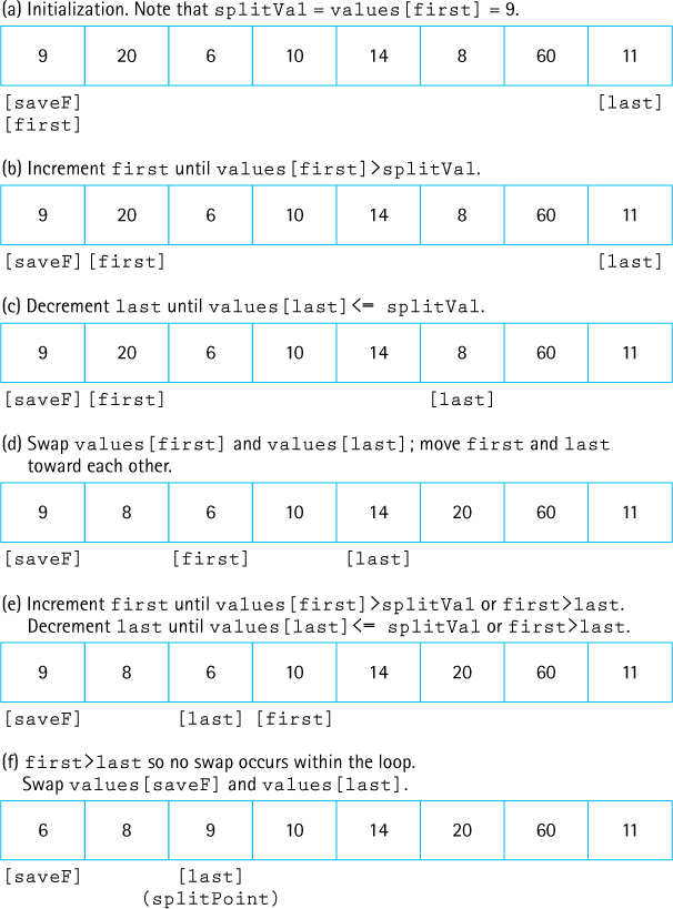
Figure 11.13 The split operation
Now values[last] is compared to splitVal. If it is greater than splitVal, we continue decrementing last; otherwise, we leave last in place (Figure 11.13c). At this point, it is clear that both values[last] and values[first] are on the wrong sides of the array. The elements to the left of values[first] and to the right of values[last] are not necessarily sorted; they are just on the correct side of the array with respect to splitVal. To put values[first] and values[last] into their correct sides, we merely swap them; we then increment first and decrement last (Figure 11.13d).
Now we repeat the whole cycle, incrementing first until we encounter a value that is greater than splitVal, then decrementing last until we encounter a value that is less than or equal to splitVal (Figure 11.13e).
When does the process stop? When first and last meet each other, no further swaps are necessary. Where they meet determines the splitPoint. This is the location where splitVal belongs; so we swap values[saveF], which contains splitVal, with the element at values[last] (Figure 11.13f). The index last is returned from the method, to be used by quickSort as the splitPoint for the next pair of recursive calls.
static int split(int first, int last)
{
  int splitVal = values[first];
  int saveF = first;
  boolean onCorrectSide;

  first++;
  do
  {
    onCorrectSide = true;
    while (onCorrectSide)       // move first toward last
      if (values[first] > splitVal)
        onCorrectSide = false;
      else
      {
        first++;
        onCorrectSide = (first <= last);
      }

    onCorrectSide = (first <= last);
    while (onCorrectSide)       // move last toward first
      if (values[last] <= splitVal)
        onCorrectSide = false;
      else
      {
      last--;
      onCorrectSide = (first <= last);
      }

    if (first < last)
    {
      swap(first, last);
      first++;
      last--;
    }
  } while (first <= last);

  swap(saveF, last);
  return last;
}
What happens if our splitting value is the largest value or the smallest value in the segment? The algorithm still works correctly, but because the split is lopsided, it is not so quick.
Is this situation likely to occur? That depends on how we choose our splitting value and on the original order of the data in the array. If we use values[first] as the splitting value and the array is already sorted, then every split is lopsided. One side contains one element, whereas the other side contains all but one of the elements. Thus our quickSort method is not a “quick” sort. Our splitting algorithm works best for an array in random order.
It is not unusual, however, to want to sort an array that is already in nearly sorted order. If this is the case, a better splitting value would be the middle value:
values[(first + last) / 2]
This value could be swapped with values[first] at the beginning of the method. It is also possible to sample three or more values in the subarray being sorted and to use their median. In some cases this will help prevent lopsided splits.
Analyzing quickSort
The analysis of quickSort is very similar to that of mergeSort. On the first call, every element in the array is compared to the dividing value (the “split value”), so the work done is O(N). The array is divided into two subarrays (not necessarily halves), which are then examined.
Each of these pieces is then divided in two, and so on. If each piece is split approximately in half, there are O(log2N) levels of splits. At each level, we make O(N) comparisons. Thus, the quick sort is also an O(N log2N) algorithm, which is quicker than the O(N2) sorts we discussed at the beginning of this chapter.
But the quick sort is not always quicker. We have log2N levels of splits if each split divides the segment of the array approximately in half. As we have seen, the array division of the quick sort is sensitive to the order of the data—that is, to the choice of the splitting value.
What happens if the array is already sorted when our version of quickSort is called? The splits are very lopsided, and the subsequent recursive calls to quickSort break our data into a segment containing one element and a segment containing all the rest of the array. This situation produces a sort that is not at all quick. In fact, there are N – 1 levels; in this case, the complexity of the quick sort is O(N2).
Such a situation is very unlikely to occur by chance. By way of analogy, consider the odds of shuffling a deck of cards and coming up with a sorted deck. Of course, in some applications we may know that the original array is likely to be sorted or nearly sorted. In such cases we would want to use either a different splitting algorithm or a different sort—maybe even shortBubble!
What about space requirements? A quick sort does not require an extra array, as a merge sort does. Are there any extra space requirements, besides the few local variables? Yes—recall that the quick sort uses a recursive approach. Many levels of recursion may be “saved” on the system stack at any time. On average, the algorithm requires O(log2N) extra space to hold this information and in the worst case requires O(N) extra space, the same as a merge sort.
Heap Sort
In each iteration of the selection sort, we searched the array for the next-smallest element and put it into its correct place in the array. Another way to write a selection sort is to find the maximum value in the array and swap it with the last array element, then find the next-to-largest element and put it into its place, and so on. Most of the work involved in this sorting algorithm comes from searching the remaining part of the array in each iteration, looking for the maximum value.
In Chapter 9, we discussed the heap, a data structure with a very special feature: We always know where to find its largest element. Because of the order property of heaps, the maximum value of a heap is in the root node. We can take advantage of this situation by using a heap to help us sort data. The general approach of the heap sort is as follows:
Take the root (maximum) element off the heap, and put it into its place.
Reheap the remaining elements. (This puts the next-largest element into the root position.)
Repeat until there are no more elements.
The first part of this algorithm sounds a lot like the selection sort. What makes the heap sort rapid is the second step: finding the next-largest element. Because the shape property of heaps guarantees a binary tree of minimum height, we make only O(log2N) comparisons in each iteration, as compared with O(N) comparisons in each iteration of the selection sort.
Building a Heap
By now you are probably protesting that we are dealing with an unsorted array of elements, not a heap. Where does the original heap come from? Before we go on, we have to convert the unsorted array, values, into a heap.
Look at how the heap relates to our array of unsorted elements. In Chapter 9, we saw how heaps can be represented in an array with implicit links. Because of the shape property, we know that the heap elements take up consecutive positions in the array. In fact, the unsorted array of data elements already satisfies the shape property of heaps. Figure 11.14 shows an unsorted array and its equivalent tree.
We also need to make the unsorted array elements satisfy the order property of heaps. First, we need to discover whether any part of the tree already satisfies the order property. All of the leaf nodes (subtrees with only a single node) are heaps. In Figure 11.15a, the subtrees whose roots contain the values 19, 7, 3, 100, and 1 are heaps because they consist solely of root nodes.
Now let us look at the first nonleaf node, the one containing the value 2 (Figure 11.15b). The subtree rooted at this node is not a heap, but it is almost a heap—all of the nodes except the root node of this subtree satisfy the order property. We know how to fix this problem. In Chapter 9, we developed a heap utility method, reheapDown, that we can use to handle this same situation. Given a tree whose elements satisfy the order property of heaps, except that the tree has an empty root, and a value to insert into the heap, reheapDown rearranges the nodes, leaving the (sub)tree containing the new element as a heap. We can just invoke reheapDown on the subtree, passing it the current root value of the subtree as the element to be inserted.

Figure 11.14 An unsorted array and its tree
We apply this method to all the subtrees on this level, and then we move up a level in the tree and continue reheaping until we reach the root node. After reheapDown has been called for the root node, the entire tree should satisfy the order property of heaps. Figure 11.15 illustrates this heap-building process; Figure 11.16 shows the changing contents of the array.
In Chapter 9, we defined reheapDown as a private method of the Heap class. There, the method had only one parameter: the element being inserted into the heap. It always worked on the entire tree; that is, it always started with an empty node at index 0 and assumed that the last tree index of the heap was lastIndex. Here, we use a slight variation: reheapDown is a static method of our Sorts class that takes a second parameter—the index of the node that is the root of the subtree that is to be made into a heap. This is an easy change; if we call the parameter root, we simply add the following statement to the beginning of the reheapDown method:
int hole = root; // Current index of hole
The algorithm for building a heap is summarized here:
We know where the root node is stored in our array representation of heaps: values[0]. Where is the first nonleaf node? From our knowledge of the array-based representation of a complete binary tree we know the first nonleaf node is found at position SIZE/2 - 1.

Figure 11.15 The heap-building process
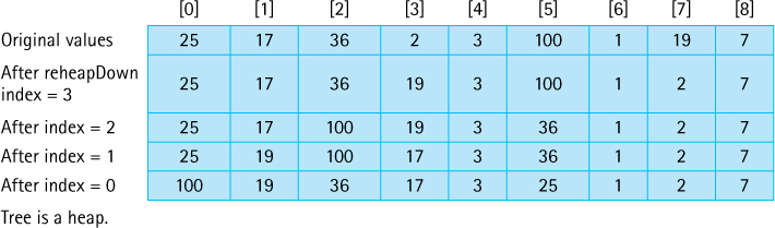
Figure 11.16 Changing contents of the array
During this heap construction the furthest any node moves is equal to its distance from a leaf. The sum of these distances in a complete tree is O(N), so building a heap in this manner is an O(N) operation.
Sorting Using the Heap
Now that we are satisfied that we can turn the unsorted array of elements into a heap, let us take another look at the sorting algorithm.
We can easily access the largest element from the original heap—it is in the root node. In our array representation of heaps, the location of the largest element is values[0]. This value belongs in the last-used array position values[SIZE - 1], so we can just swap the values in these two positions. Because values[SIZE - 1] now contains the largest value in the array (its correct sorted value), we want to leave this position alone. Now we are dealing with a set of elements, from values[0] through values[SIZE - 2], that is almost a heap. We know that all of these elements satisfy the order property of heaps, except (perhaps) the root node. To correct this condition, we call our heap utility, reheapDown. (But our original reheapDown method assumed that the heap’s tree ends at position lastIndex. We must again redefine reheapDown, so that it now accepts three parameters, with the third being the ending index of the heap. Once again the change is easy; the new code for reheapDown is included in the Sorts class.)
After reheapDown returns we know that the next-largest element in the array is in the root node of the heap. To put this element in its correct position, we swap it with the element in values[SIZE - 2]. Now the two largest elements are in their final correct positions, and the elements in values[0] through values[SIZE - 3] are almost a heap. We call reheapDown again, and now the third-largest element is in the root of the heap.
We repeat this process until all of the elements are in their correct positions—that is, until the heap contains only a single element, which must be the smallest element in the array, in values[0]. This is its correct position, so the array is now completely sorted from the smallest to the largest element. At each iteration, the size of the unsorted portion (represented as a heap) gets smaller and the size of the sorted portion gets larger. When the algorithm ends, the size of the sorted portion is the size of the original array.
The heap sort algorithm, as we have described it here, sounds like a recursive process: each time, we swap and reheap a smaller portion of the total array. Because it uses tail recursion, we can code the repetition just as clearly using a simple for loop. The node-sorting algorithm is as follows:
Method heapSort first builds the heap and then sorts the nodes, using the algorithms just discussed.
static void heapSort()
// Post: The elements in the array values are sorted by key
{
  int index;
  // Convert the array of values into a heap
  for (index = SIZE/2 - 1; index >= 0; index--)
    reheapDown(values[index], index, SIZE - 1);

  // Sort the array
  for (index = SIZE - 1; index >=1; index--)
  {
    swap(0, index);
    reheapDown(values[0], 0, index - 1);
  }
}
Figure 11.17 shows how each iteration of the sorting loop (the second for loop) would change the heap created in Figure 11.16. Each line represents the array after one operation. The sorted elements are shaded.

Figure 11.17 Effect of heapSort on the array
We entered the heapSort method with a simple array of unsorted values and returned with an array of the same values sorted in ascending order. Where did the heap go? The heap in heapSort is just a temporary structure, internal to the sorting algorithm. It is created at the beginning of the method to aid in the sorting process, but then is methodically diminished element by element as the sorted part of the array grows. When the method ends, the sorted part fills the array and the heap has completely disappeared. When we used heaps to implement priority queues in Chapter 9, the heap structure stayed around for the duration of the use of the priority queue. The heap in heapSort, by contrast, is not a retained data structure. It exists only temporarily, during the execution of the heapSort method.

Analyzing heapSort
The code for method heapSort is very short—only a few lines of new code plus the helper method reheapDown, which we developed in Chapter 9 (albeit slightly revised). These few lines of code, however, do quite a bit of work. All of the elements in the original array are rearranged to satisfy the order property of heaps, moving the largest element up to the top of the array, only to put it immediately into its place at the bottom. It is hard to believe from a small example such as the one in Figures 11.16 and 11.17 that heapSort is very efficient.
In fact, for small arrays, heapSort is not very efficient because of its “overhead.” For large arrays, however, heapSort is very efficient. Consider the sorting loop. We loop through N – 1 times, swapping elements and reheaping. The comparisons occur in reheapDown (actually in its helper method newHole). A complete binary tree with N nodes has ⌊log2N⌋ levels. In the worst case, if the root element had to be bumped down to a leaf position, the reheapDown method would make O(log2N) comparisons. Thus method reheapDown is O(log2N). Multiplying this activity by the N – 1 iterations shows that the sorting loop is O(N log2N).
Combining the original heap build that is O(N), and the sorting loop, we can see that the heap sort requires O(N log2N) comparisons. Unlike the quick sort, the heap sort’s efficiency is not affected by the initial order of the elements. Even in the worst case it is O(N log2N). A heap sort is just as efficient in terms of space; only one array is used to store the data. The heap sort requires only constant extra space.
The heap sort is an elegant, fast, robust, space-efficient algorithm!
11.4 More Sorting Considerations
This section wraps up our coverage of sorting by revisiting testing and efficiency, considering the “stability” of sorting algorithms, and discussing special concerns involved with sorting objects rather than primitive types.
Testing
All of our sorts are implemented within the test harness presented in Section 11.1, “Sorting.” That test harness program, Sorts, allows us to generate a random array of size 50, sort it with one of our algorithms, and view the sorted array. It is easy to determine whether the sort was successful. If we do not want to verify success by eyeballing the output, we can always use a call to the isSorted method of the Sorts class.
The Sorts program is a useful tool for helping evaluate the correctness of our sorting methods. To thoroughly test them, however, we should vary the size of the array they are sorting. A small revision to Sorts, allowing the user to pass the array size as a command line parameter, would facilitate this process. We should also vary the original order of the array—for example, test an array that is in reverse order, one that is almost sorted, and one that has all identical elements (to make sure we do not generate an “array index out of bounds” error).
Besides validating that our sort methods create a sorted array, we can check their performance. At the start of the sorting phase we can initialize two variables, numSwaps and numCompares, to 0. By carefully placing statements incrementing these variables throughout our code, we can use them to track how many times the code performs swaps and comparisons. Once we output these values, we can compare them to the predicted theoretical values. Inconsistencies would require further review of the code (or maybe the theory!).
Efficiency
When N Is Small
As emphasized throughout this chapter, our analysis of efficiency relies on the number of comparisons made by a sorting algorithm. This number gives us a rough estimate of the computation time involved. The other activities that accompany the comparison (swapping, keeping track of boolean flags, and so forth) contribute to the “constant of proportionality” of the algorithm.
In comparing order of growth evaluations, we ignored constants and smaller-order terms because we want to know how the algorithm performs for large values of N. In general, an O(N2) sort requires few extra activities in addition to the comparisons, so its constant of proportionality is fairly small. Conversely, an O(N log2N) sort may be more complex, with more overhead and thus a larger constant of proportionality. This situation may cause anomalies in the relative performances of the algorithms when the value of N is small. In this case, N2 is not much greater than N log2N, and the constants may dominate instead, causing an O(N2) sort to run faster than an O(N log2N) sort. A programmer can leverage this fact to improve the running time of sort code, by having the code switch between an O(N log2N) sort for large portions of the array and an O(N2) sort for small portions.
We have discussed sorting algorithms that have complexity of either O(N2) or (N log2N). Now we ask an obvious question: Do algorithms that are better than (N log2N) exist? No, it has been proven theoretically that we cannot do better than (N log2N) for sorting algorithms that are based on comparing keys—that is, on pairwise comparison of elements.
Eliminating Calls to Methods
Sometimes it may be desirable, for efficiency reasons, to streamline the code as much as possible, even at the expense of readability. For instance, we have consistently used
swap(index1, index2);
when we wanted to swap two elements in the values array. We would achieve slightly better execution efficiency by dropping the method call and directly coding
tempValue = values[index1];
values[index1] = values[index2];
values[index2] = tempValue;
Coding the swap operation as a method made the code simpler to write and to understand, avoiding a cluttered sort method. However, method calls require extra overhead that we may prefer to avoid during a real sort, where the method is called over and over again within a loop.
The recursive sorting methods, mergeSort and quickSort, bring up a similar situation: They require the extra overhead involved in executing the recursive calls. We may want to avoid this overhead by coding nonrecursive versions of these methods.
In some cases, an optimizing compiler replaces method calls with the inline expansion of the code of the method. In that case, we get the benefits of both readability and efficiency.
Programmer Time
If the recursive calls are less efficient, why would anyone ever decide to use a recursive version of a sort? This decision involves a choice between types of efficiency. Until now, we have been concerned only with minimizing computer time. While computers are becoming faster and cheaper, however, it is not at all clear that computer programmers are following that trend. In fact, programmers are becoming more expensive. Therefore, in some situations, programmer time may be an important consideration in choosing an algorithm and its implementation. In this respect, the recursive version of the quick sort is more desirable than its nonrecursive counterpart, which requires the programmer to simulate recursion.
If a programmer is familiar with a language’s support library, the programmer can use the sort routines provided there. The Arrays class in the Java library’s util package defines a number of sorts for sorting arrays. Likewise, the Java Collections Framework, which was introduced in Section 2.10, “Stack Variations,” provides methods for sorting many of its collection objects.
Space Considerations
Another efficiency consideration is the amount of memory space required. In small applications, memory space is not a very important factor in choosing a sorting algorithm. In large applications, such as a database with many gigabytes of data, space may pose a serious concern. We looked at only two sorts, mergeSort and quickSort, that required more than constant extra space. The usual time versus space trade-off applies to sorts: More space often means less time, and vice versa.
Because processing time is the factor that applies most often to sorting algorithms, we have considered it in detail here. Of course, as in any application, the programmer must determine the program’s goals and requirements before selecting an algorithm and starting to code.
Objects and References
So that we could concentrate on the algorithms, we limited our implementations to sorting arrays of integers. Do the same approaches work for sorting objects? Of course, although a few special considerations apply.
Keep in mind that when we sort an array of objects, we are manipulating references to the objects, not the objects themselves (Figure 11.18). This point does not affect any of our algorithms, but it is still important to understand. For example, if we decide to swap the objects at index 0 and index 1 of an array, it is actually the references to the objects that we swap, not the objects themselves. In one sense, we view objects, and the references to the objects, as identical, because using a reference is the only way we can access an object.

Figure 11.18 Sorting arrays with references
Comparing Objects
When sorting objects, we must have a way to compare two objects and decide which is “larger.” Two basic approaches are used when dealing with Java objects, both of which you are familiar with from previous chapters. If the object class exports a compareTo operation, or something similar, it can be used to provide the needed comparison.
As we have seen, the Java library provides another interface related to comparing objects, a generic interface called Comparator. A programmer can define more than one Comparator for a class, allowing more flexibility.
Any sort implementation must compare elements. Our sorting methods so far have used built-in integer comparison operations such as < or <=. If we sort Comparable objects instead of integers, we could use the compareTo method that is guaranteed to exist by that interface. Alternatively, we could use the versatile approach supported by the Comparator interface. If we pass a Comparator object comp to a sorting method as a parameter, the method can use comp.compare to determine the relative order of two objects and base its sort on that relative order. Passing a different Comparator object results in a different sorting order. Perhaps one Comparator object defines an increasing order, and another defines a decreasing order. Or perhaps the different Comparator objects could define order based on different attributes of the objects. Now, with a single sorting method, we can produce many different sort orders.
Stability
The stability of a sorting algorithm is based on what it does with duplicate values. Of course, the duplicate values all appear consecutively in the final order. For example, if we sort the list A B B A, we get A A B B. But is the relative order of the duplicates the same in the final order as it was in the original order? If that property is guaranteed, we have a stable sort.
In our descriptions of the various sorts, we showed examples of sorting arrays of integers. Stability is not important when sorting primitive types. If we sort objects, however, the stability of a sorting algorithm can become more important. We may want to preserve the original order of unique objects considered identical by the comparison operation.
Suppose the elements in our array are student objects with instance values representing their names, postal codes, and identification numbers. The list may normally be sorted by the unique identification numbers. For some purposes we might want to see a listing in order by name. In this case the comparison would be based on the name variable. To sort by postal code, we would sort on that instance variable.
If the sort is stable, we can get a listing by postal code, with the names in alphabetical order within each postal code, by sorting twice: the first time by name and the second time by postal code. A stable sort preserves the order of the elements when it finds a match. The second sort, by postal code, produces many such matches, but the alphabetical order imposed by the first sort is preserved.
Of the various types of sorts that we have discussed in this text, only heapSort and quickSort are inherently unstable. The stability of the other sorts depends on how the code handles duplicate values. In some cases, stability depends on whether a < or a <= comparison is used in some crucial comparison statement. In the exercises at the end of this chapter, you are asked to examine the code for the various sorts and determine whether they are stable.
If we can directly control the comparison operation used by our sort method, we can allow more than one variable to be used in determining a sort order. Thus another, more efficient approach to sorting our students by ZIP code and name is to define an appropriate compareTo method for determining sort order as follows (for simplicity, this code assumes we can directly compare the name values):
if (postalcode < other.postalcode)
  return -1;
else
if (postalcode > other.postalcode)
  return +1;
else
// Postal codes are equal
if (name < other.name)
  return -1;
else
if (name > other.name)
  return +1;
else
  return 0;
With this approach we need to sort the array only once.
11.5 Searching
This section reviews material scattered throughout the text related to searching. Here we bring these topics together to be considered in relationship to each other to gain an overall perspective. Searching is a crucially important information processing activity. Options are closely related to the way data is structured and organized.
Sometimes access to a needed element stored in a collection can be achieved directly. For example, with both our array-based and link-based stack ADT implementations, we can directly access the top element on the stack; the top method is O(1). Access to our array-based indexed lists, given a position on the list, is also direct; O(1) time is needed. Often, however, direct access is not possible, especially when we want to access an element based on its value. For instance, if a list contains student records, we may want to find the record of the student named Suzy Brown or the record of the student whose ID number is 203557. In such cases, some kind of searching technique is needed to allow retrieval of the desired record.
In this section we look at some of the basic “search by value” techniques for collections. Most of these techniques were encountered previously in the text—sequential search in Section 1.6, binary search in Sections 1.6 and 3.3, and hashing in Section 8.4.
Sequential Searching
We cannot discuss efficient ways to find an element in a collection without considering how the elements were added into the collection. Therefore, our discussion of search algorithms is related to the issue of a collection’s add operation. Suppose that we want to add elements as quickly as possible, and are not overly concerned about how long it takes to find them. We would put the element into the last slot in an array-based collection or the first slot in a linked collection. Both are O(1) insertion algorithms. The resulting collection is sorted according to the time of insertion, not according to key value.
To search this collection for the element with a given key, we must use a simple sequential (or linear) search. For example, we used a sequential search for the find method of our ArrayCollection class in Chapter 5. Beginning with the first element in the collection, we search for the desired element by examining each subsequent element’s key until either the search is successful or the collection is exhausted.
Based on the number of comparisons, this search is O(N), where N represents the number of elements. In the worst case, in which we are looking for the last element in the collection or for a nonexistent element, we will make N key comparisons. On average, assuming that there is an equal probability of searching for any element in the collection, we will make N/2 comparisons for a successful search; that is, on average we must search half of the collection.
High-Probability Ordering
The assumption of equal probability for every element in the collection is not always valid. Sometimes certain collection elements are in much greater demand than others. This observation suggests a way to improve the search: Put the most-often-desired elements at the beginning of the collection.1 Using this scheme, we are more likely to make a hit in the first few tries, and rarely do we have to search the whole collection.
If the elements in the collection are not static or if we cannot predict their relative demand, we need some scheme to keep the most frequently used elements at the front of the collection. One way to accomplish this goal is to move each element accessed to the front of the collection. Of course, there is no guarantee that this element is later frequently used. If the element is not retrieved again, however, it drifts toward the end of the collection as other elements move to the front. This scheme is easy to implement for linked collections, requiring only a few pointer changes. It is less desirable for collections kept sequentially in arrays, because we need to move all the other elements down to make room at the front.
An alternative approach, which causes elements to move toward the front of the collection gradually, is appropriate for either linked or array-based collection representations. As an element is found, it is swapped with the element that precedes it. Over many collection retrievals, the most frequently desired elements tend to be grouped at the front of the collection. To implement this approach, we need to modify only the end of the algorithm to exchange the found element with the one before it in the collection (unless it is the first element). This change should be documented; it is an unexpected side effect of searching the collection.
Keeping the most active elements at the front of the collection does not affect the worst case; if the search value is the last element or is not in the collection, the search still takes N comparisons. It is still an O(N) search. However, the average performance on successful searches should improve. Both of these high-probability ordering algorithms depend on the assumption that some elements in the collection are used much more often than others. If this assumption is erroneous, a different ordering strategy is needed to improve the efficiency of the search technique.
Collections in which the relative positions of the elements are changed in an attempt to improve search efficiency are called self-organizing or self-adjusting collections.
Sorted Collections
As discussed in Section 1.6, “Comparing Algorithms,” if a collection is sorted, we can write more efficient search routines.
First of all, if the collection is sorted, a sequential search no longer needs to search the whole collection to discover that an element does not exist. It just needs to search until it has passed the element’s logical place in the collection—that is, until it encounters an element with a larger key value.
Therefore, one advantage of sequential searching a sorted collection is the ability to stop searching before the collection is exhausted if the element does not exist. Again, the search is O(N)—the worst case, searching for the largest element, still requires N comparisons. The average number of comparisons for an unsuccessful search is now N/2, however, instead of a guaranteed N.
Another advantage of sequential searching is its simplicity. The disadvantage is its performance: In the worst case we have to make N comparisons. If the collection is sorted and stored in an array, we can improve the search time to a worst case of O(log2N) by using a binary search (see Section 1.6, “Comparing Algorithms”). This improvement in efficiency, however, comes at the expense of simplicity.
The binary search is not guaranteed to be faster for searching very small collections. Even though such a search generally requires fewer comparisons, each comparison involves more computation. When N is very small, this extra work (the constants and smaller terms that we ignore in determining the order of growth approximation) may dominate. For instance, in one assembly-language program, the sequential search required 5 time units per comparison, whereas the binary search took 35. For a collection size of 16 elements, therefore, the worst-case sequential search would require 5 * 16 = 80 time units. The worst-case binary search requires only 4 comparisons, but at 35 time units each, the comparisons take 140 time units. In cases where the number of elements in the collection is small, a sequential search is certainly adequate and sometimes faster than a binary search.
As the number of elements increases, the magnitude of the difference between the sequential search and the binary search grows very quickly. Look back at the Vocabulary Density experiment results in Table 5.1 on page 324 for an example of this effect.
The binary search discussed here is appropriate only for collection elements stored in a sequential array-based representation. After all, how can we efficiently find the midpoint of a linked collection? We already know one structure that allows us to perform a binary search on a linked data representation: the binary search tree. The operations used to search a binary tree were discussed in Chapter 7.
Hashing
So far, we have succeeded in paring down our O(N) search to a complexity of O(log2N) by keeping the collection sorted sequentially with respect to the key value. That is, the key in the first element is less than (or equal to) the key in the second element, which is less than (or equal to) the key in the third, and so on. Can we do better than that? Is it possible to design a search of O(1)—that is, one with a constant search time, no matter where the element is in the collection? Yes, the hash table approach to storage presented in Sections 4 through 6 of Chapter 8 allows constant search time in many situations.
If our hash function is efficient, never produces duplicates and the hash table size is large compared to the expected number of entries in the collection, then we have reached our goal—constant search time. In general, this is not the case, although in many practical situations it is possible.
Clearly, as the number of entries in a collection approaches the size of the hash table’s internal array, the efficiency of the hash table deteriorates. This is why the load of the hash table is monitored. If the table needs to be resized and the entries all rehashed there is a one-time heavy cost incurred.
As discussed in Chapter 8, a precise analysis of the complexity of hashing is difficult. It depends on the domain and distribution of keys, the hash function, the size of the table, and the collision resolution policy. In practice it is usually not difficult to achieve close to O(1) efficiency using hashing. For any given application area it is possible to test variations of hashing schemes to see which works best.
Summary
We have not attempted in this chapter to describe every known sorting algorithm. Instead, we presented a few of the popular sorts, of which many variations exist. It should be clear from this discussion that no single sort is best for all applications. The simpler, generally O(N2) sorts work as well as, and sometimes better than, the more complicated sorts for fairly small values of N. Because they are simple, these sorts require relatively little programmer time to write and maintain. As we add features to improve sorts, we also increase the complexity of the algorithms, expanding both the work required by the routines and the programmer time needed to maintain them.
Another consideration in choosing a sort algorithm is the order of the original data. If the data are already sorted (or almost sorted), shortBubble is O(N), whereas some versions of quickSort are O(N2).
As always, the first step in choosing an algorithm is to determine the goals of the particular application. This effort usually narrows the choice of options considerably. After that, knowledge of the strong and weak points of the various algorithms assists us in selecting a sorting method.
Table 11.3 compares the sorts discussed in this chapter in terms of O notation. Searching, similar to sorting, is a topic that is closely tied to the goal of efficiency. We speak of a sequential search of a collection as an O(N) search, because it may require as many as N comparisons to locate an element. (N refers to the number of elements in the collection.) Binary searches are considered to be O(log2N) and are appropriate for array-based collections if they are sorted. A binary search tree may be used to allow binary searches on a linked structure. The goal of hashing is to produce a search that approaches O(1) time efficiency. Because of collisions of hash locations, some searching is usually necessary. A good hash function minimizes collisions and distributes the elements randomly throughout the table.
Table 11.3 Comparison of Sorting Algorithms
| Order of Growth | |||
|---|---|---|---|
| Sort | Best Case | Average Case | Worst Case |
selectionSort |
O(N2) | O(N2) | O(N2) |
bubbleSort |
O(N2) | O(N2) | O(N2) |
shortBubble |
O(N)* | O(N2) | O(N2) |
insertionSort |
O(N)* | O(N2) | O(N2) |
mergeSort |
O(N log2N) | O(N log2N) | O(N log2N) |
quickSort |
O(N log2N) | O(N log2N) | O(N2) (depends on split) |
heapSort |
O(N log2N) | O(N log2N) | O(N log2N) |
* Data almost sorted. |
|||
In the chapter introduction we addressed the fact that modern programming environments usually provide predefined sort and search facilities. Professional programmers usually use these packaged sort and search tools when they need to sort/search data. Nevertheless, as a student of computing, it is good for you to become familiar with basic sorting and searching techniques.
Exercises
11.1 Sorting
-
 A test harness program for testing sorting methods is provided with the program files. It is in the file
 Sorts.javain thech11.sortspackage. The program includes a swap method that is used by all of the sorting methods to swap array elements.Describe an approach to modifying the program so that after calling a sorting method the program prints out the number of swaps needed by the sorting method.
Implement your approach.
Test your new program by running the
selectionSortmethod. Your program should report 49 swaps.
11.2 Simple Sorts
-
Determine the order of growth complexity for the selection sort based on the number of elements moved rather than on the number of comparisons
For the best case.
For the worst case.
-
In what case(s), if any, is the complexity of the selection sort O(log2N)?
-
 Write a version of the bubble sort algorithm that sorts a list of integers in descending order.
 -
In what case(s), if any, is the complexity of the bubble sort O(N)?
-
How many comparisons would be needed to sort an array containing 100 elements using
shortBubblein the worst case?
in the best case?
-
Show the contents of the array

after the fourth iteration of
selectionSort.bubbleSort.insertionSort.
-
For each of the sorting algorithms presented in Section 11.2 (selection sort, bubble sort, short bubble, and insertion sort) how many comparisons would be needed to sort an array containing 100 elements if the original array values
were already sorted?
were sorted in reverse order?
were all identical?
-
Repeat Exercise 8 but report the number of “swaps.”
-
In Exercise 1 you were asked to modify the
Sortsprogram so that it would output the number of swaps used by a sorting method. It is a little more difficult to have the program also output the number of comparisons (compares) needed. You must include one or more statements to increment your counter within the sorting methods themselves. For each of the listed methods, make and test the changes needed, and list both the number of swaps and the number of compares needed by theSortsprogram to sort an array of 50 random integers.selectionSortswaps: ____ compares: ____ bubbleSortswaps: ____ compares: ____ shortBubbleswaps: ____ compares: ____ insertionSortswaps: ____ compares: ____
11.3 O(N log2N) Sorts
-
A merge sort is used to sort an array of 1,000 test scores in descending order. Which one of the following statements is true?
The sort is fastest if the original test scores are sorted from smallest to largest.
The sort is fastest if the original test scores are in completely random order.
The sort is fastest if the original test scores are sorted from largest to smallest.
The sort is the same, no matter what the order of the original elements.
-
Show how the values in the array in Exercise 7 would be arranged immediately before the execution of method
mergein the original (nonrecursive) call tomergeSort. -
Determine the order of growth complexity for
mergeSortbased on the number of elements moved rather than on the number of comparisonsfor the best case.
for the worst case.
-
Use the Three-Question Method to verify
mergeSort. -
In what case(s), if any, is the complexity of the quick sort O(N2)?
-
Which is true about the quick sort?
A recursive version executes faster than a nonrecursive version.
A recursive version has fewer lines of code than a nonrecursive version.
A nonrecursive version takes more space on the run-time stack than a recursive version.
It can be programmed only as a recursive function.
-
Determine the order of growth complexity for
quickSortbased on the number of elements moved rather than on the number of comparisonsfor the best case.
for the worst case.
-
Use the Three-Question Method to verify
quickSort. -
Using the algorithms for creating a heap and sorting an array using a heap-based approach:
Show how the values in the array in Exercise 7 would have to be rearranged to satisfy the heap property.
Show how the array would look with four values in the sorted portion after reheaping.
-
A sorting function is called to sort a list of 100 integers that have been read from a file. If all 100 values are zero, what would the execution costs (in terms of O notation) be if the sort used was
mergeSort?quickSort, with the first element used as the split value?heapSort?
-
Suppose a list is already sorted from smallest to largest when a sort is called.
Which of the following sorts would take the longest time to execute and which would take the shortest time?
quickSort, with the first element used as the split valueshortBubbleselectionSortheapSortinsertionSortmergeSort
-
A very large array of elements is to be sorted. The program will be run on a personal computer with limited memory. Which sort would be a better choice: a heap sort or a merge sort? Why?
-
True or False? Explain your answers.
mergeSortrequires more space to execute thanheapSort.quickSort(using the first element as the split value) is better for nearly sorted data thanheapSort.The efficiency of
heapSortis not affected by the original order of the elements.
-
In Exercise 1 you were asked to modify the
Sortsprogram so that it would output the number of swaps used by a sorting method. It is a little more difficult to have the program also output the number of comparisons needed. You must include one or more statements to increment your counter within the sorting methods themselves. For each of the listed methods, make and test the changes needed, and list the number of comparisons needed bySortsto sort an array of 50 random integers.mergeSortcompares: ____ quicksortcompares: ____ heapSortcompares: ____
11.4 More Sorting Considerations
-
For small values of N, the number of steps required for an O(N2) sort might be less than the number of steps required for a sort of a lower degree. For each of the following pairs of mathematical functions f and g below, determine a value N such that if n > N, g(n) > f(n). This value represents the cutoff point, above which the O(n2) function is always larger than the other function.
f (n) = 4n g(n) = n2 + 1 f (n) = 3n + 20 g(n) = ½ n2 + 2 f (n) = 4 log2n + 10 g(n) = n2 f (n) = 100 log2n g(n) = n2 f (n) = 1000 log2n g(n) = n2
-
Give arguments for and against using methods (such as
swap) to encapsulate frequently used code in a sorting routine. -
What is meant by this statement: “Programmer time is an efficiency consideration.” Give an example of a situation in which programmer time is used to justify the choice of an algorithm, possibly at the expense of other efficiency considerations.
-
Go through the sorting algorithms coded in this chapter and determine which ones are stable as coded. Identify the key statement in the corresponding method that determines the stability.
-
We said that the heap sort algorithm is inherently unstable. Explain why.
-
Which sorting algorithm would you not use under each of the following conditions?
The sort must be stable.
Space is very limited.
11.5 Searching
-
Fill in the following table, showing the number of comparisons needed either to find the value or to determine that the value is not in the indicated structure based on the given approach and given the following values:

-
If you know the index of an element stored in an array of N unsorted elements, which of the following best describes the order of the algorithm to find the element?
O(1)
O(N)
O(log2N)
O(N2)
O(0.5N)
-
The element being searched for is not in an array of 100 elements. What is the average number of comparisons needed in a sequential search to determine that the element is not there
if the elements are completely unsorted?
if the elements are sorted from smallest to largest?
if the elements are sorted from largest to smallest?
-
The element being searched for is not in an array of 100 elements. What is the maximum number of comparisons needed in a sequential search to determine that the element is not there
if the elements are completely unsorted?
if the elements are sorted from smallest to largest?
if the elements are sorted from largest to smallest?
-
The element being searched for is in an array of 100 elements. What is the average number of comparisons needed in a sequential search to determine the position of the element
if the elements are completely unsorted?
if the elements are sorted from smallest to largest?
if the elements are sorted from largest to smallest?
-
Choose the answer that correctly completes the following sentence: The elements in an array may be sorted by highest probability of being requested to reduce
the average number of comparisons needed to find an element in the list.
the maximum number of comparisons needed to detect that an element is not in the list.
the average number of comparisons needed to detect that an element is not in the list.
the maximum number of comparisons needed to find an element that is in the list.
-
True or False? Explain your answers.
A binary search of a sorted set of elements in an array is always faster than a sequential search of the elements.
A binary search is an O(N log2N) algorithm.
A binary search of elements in an array requires that the elements be sorted from smallest to largest.
A high-probability ordering scheme would be a poor choice for arranging an array of elements that are equally likely to be requested.
-
How might you order the elements in a list of Java’s reserved words to use the idea of high-probability ordering?