
CHAPTER 7: The Binary Search Tree ADT
© Ake13bk/Shutterstock
Chapter 5 introduced the Collection ADT with core operations add, remove, get, and contains. Chapter 6 presented the List ADT—a list is a collection that also supports iteration and indexing. In this chapter we present another variation of a collection. The distinguishing features of a binary search tree are that it maintains its elements in increasing order and it provides, in the general case, efficient implementations of all the core operations. How can it do this?
The binary search tree can be understood by comparing a sorted linked list to a sorted array:

Consider the steps needed to add the value 985 to each of these structures. For the linked list we must perform a linear search of the structure in order to find the point of insertion. That is an O(N) operation. However, once the insertion point is discovered, we can add the new value by creating a new node and rearranging a few references, an O(1) operation. On the other hand, the sorted array supports the binary search algorithm (see Sections 1.6 and 3.3, “Comparing Algorithms: Order of Growth Analysis” and “Recursive Processing of Arrays”) allowing us to quickly find the point of insertion, an O(log2N) operation. Even though we quickly find the insertion point we still need to shift all the elements “to the right” of the location one index higher in the array, an O(N) operation. In summation, the linked list exhibits a slow find but a fast insertion, whereas the array is the opposite, a fast find but a slow insertion.
Can we combine the fast search of the array with the fast insertion of the linked list? The answer is yes!—with a binary search tree. A binary search tree is a linked structure that allows for quick insertion (or removal) of elements. But instead of one link per node it uses two links per node as shown below on the right where we display the sorted list 5, 8, 12, 20, and 27 as a binary search tree, along with equivalent array and linked list representations.

As you will see in this chapter, the availability of two links allows us to embed a binary search within the linked structure, thus combining fast binary search with fast node insertion—the best of both worlds. The binary search tree provides us with a data structure that retains the flexibility of a linked list while allowing quicker [O(log2N) in the general case] access to any node in the list.
A binary search tree is a special case of a more general data structure, the tree. Many variations of the tree structure exist. We begin this chapter with an overview of tree terminology and briefly discuss general tree implementation strategies and applications. We then concentrate on the design and use of a binary search tree.
7.1 Trees
Each node in a singly linked list may point to one other node: the one that follows it. Thus, a singly linked list is a linear structure; each node in the list (except the last) has a unique successor. A tree is a nonlinear structure in which each node is capable of having multiple successor nodes, called children. Each of the children, being nodes in a tree, can also have multiple child nodes, and these children can in turn have many children, and so on, giving the tree its branching structure. The “beginning” of the tree is a unique starting node called the root.
Trees are useful for representing lots of varied relationships. Figure 7.1 shows four example trees. The first represents the hierarchical inheritance relationship among a set of Java classes, the second shows a naturally occurring tree—a tree of cellular organisms, the third is a game tree used to analyze choices in a turn-taking game, and the fourth shows how a simply connected maze (no loops) can be represented as a tree.
Trees are recursive structures. We can view any tree node as being the root of its own tree; such a tree is called a subtree of the original tree. For example, in Figure 7.1a the node labeled “Abstract List” is the root of a subtree containing all of the Java list-related classes.
There is one more defining quality of a tree—a tree’s subtrees are disjoint; that is, they do not share any nodes. Another way of expressing this property is to say that there is a unique path from the root of a tree to any other node of the tree. In the structure below these rules are violated. The subtrees of A are not disjoint as they both contain the node D; there are two paths from the root to the node containing D. Therefore, this structure is not a tree.

As you can already see, our tree terminology borrows from both genealogy; for example, we speak of “child” nodes, and from botany, for example, we have the “root” node. Computer scientists tend to switch back and forth between these two terminological models seamlessly. Let us expand our tree vocabulary using the tree of characters in Figure 7.2 as an example.

Figure 7.1 Example trees
The root of the tree is A (from the botany point of view we usually draw our trees upside down!). The children of A are B, F, and X. Since they are A’s children it is only natural to say that A is their parent. We also say that B, F, and X are siblings. Continuing with the genealogical trend, we can speak of a node’s descendants (the children of a node, and their children, and so on recursively) and the ancestors of a node (the parent of the node, and their parent, and so on recursively). In our example, the descendants of X are H, Q, Z, and P, and the ancestors of P are H, X, and A. Obviously, the root of the tree is the ancestor of every other node in the tree, but the root node has no ancestors itself.

Figure 7.2 Sample tree

Figure 7.3 Tree terminology
A node can have many children but only a single parent. In fact, every node (except the root) must have a single parent. This is a consequence of the “all subtrees of a node are disjoint” rule—you can see that in the “not a tree” example on page 423 that D has two parents.
If a node in the tree has no children, it is called a leaf. In our example tree in Figure 7.2 the nodes C, T, F, P, Q, and Z are leaf nodes. Sometimes we refer to the nonleaf nodes as interior nodes. The interior nodes in our example are A, B, X, and H.
The level of a node refers to its distance from the root. In Figure 7.2, the level of the node containing A (the root node) is 0 (zero), the level of the nodes containing B, F, and X is 1, the level of the nodes containing C, T, H, Q, and Z is 2, and the level of the node containing P is 3. The maximum level in a tree determines its height so our example tree has a height of 3. The height is equal to the highest number of links between the root and a leaf.
Tree Traversals
To traverse a linear linked list, we set a temporary reference to the beginning of the list and then follow the list references from one node to the other, until reaching a node whose reference value is null. Similarly, to traverse a tree, we initialize our temporaryreference to the root of the tree. But where do we go from there? There are as many choices as there are children of the node being visited.
Breadth-First Traversal
Let us look at two important related approaches to traversing a general tree structure: breadth-first and depth-first. We think of the breadth of a tree as being from side-to-side and the depth of a tree as being from top-to-bottom. Accordingly, in a breadth-first traversal we first visit the root of the tree.1 Next we visit, in turn, the children of the root (typically from leftmost to rightmost), followed by visiting the children of the children of the root and so on until all of the nodes have been visited. Because we sweep across the breadth of the tree, level by level, this is also sometimes called a level-order traversal.
Figure 7.4a shows that in a breadth-first traversal of our sample tree the order the nodes are visited is A B F X C T H Q Z P. But, how can we implement this traversal? As part of visiting a node of the tree we must store references to its children so that we can visit them later in the traversal. In our example, when visiting node A, we need to store references to nodes B, F, and X. When we next visit node B we need to store references to nodes C and T—but they must be stored “behind” the previously stored F and X nodes so that nodes are visited in the desired order. What ADT supports this first in, first out (FIFO) approach? The Queue ADT. Here is a breadth-first traversal algorithm:

Figure 7.4 Tree Traversals
The Breadth-First Traversal algorithm begins by making sure the tree is not empty—if it is, no processing occurs. It is almost always a good idea to check for the degenerate case of an empty tree like this at the start of tree processing. Once it is determined that the tree is not empty, the algorithm enqueues the root node of the tree. We could just visit the root node at this point, but by enqueuing it, we set up the queue for the processing loop that follows. That loop repeatedly pulls a node off the queue, visits it, and then enqueues its children, until it runs out of nodes to process—that is, until the queue is empty.
Table 7.1 shows a trace of the algorithm on the sample tree of Figure 7.2. Trace the algorithm yourself and verify the contents of the table.
Traversal of our collection structures are needed in case we must visit every node in the structure to perform some processing. Suppose, for example, we had a tree of bank account information and wanted to sum all the amounts of all the accounts. A breadth-first traversal of the tree in order to retrieve all the account information is as good as any other traversal approach in this situation.
Besides allowing us to visit every node, for certain applications the breadth-first approach can provide additional benefits. For example, if our tree represents choices in a game (see Figure 7.1c) a breadth-first approach could provide a fast way to determine our next move. It amounts to looking at all possible next moves, and if desired all possible responses, and so on one level at a time. The point is we can avoid getting stuck traveling deeply down a tree path that represents a never-ending sequence of moves if we use breadth-first search. Using trees to represent sequences of alternatives and their ramifications, such as those found in a game, and traversing such trees using the breadth-first search to make a good choice among the alternatives, is a common artificial intelligence technique.
Table 7.1 Breadth-First Search Algorithm Trace
| After Loop Iteration | Node | Visited So Far | Queue |
|---|---|---|---|
| 0 | A | ||
| 1 | A | A | B F X |
| 2 | B | A B | F X C T |
| 3 | F | A B F | X C T |
| 4 | X | A B F X | C T H Q Z |
| 5 | C | A B F X C | T H Q Z |
| 6 | T | A B F X C T | H Q Z |
| 7 | H | A B F X C T H | Q Z P |
| 8 | Q | A B F X C T H Q | Z P |
| 9 | Z | A B F X C T H Q Z | P |
| 10 | P | A B F X C T H Q Z P | null |
Depth-First Traversal
A depth-first traversal, as might be expected, is the counterpart of the breadth-first traversal. Rather than visiting the tree level by level, expanding gradually away from the root, with a depth-first traversal we move quickly away from the root, traversing as far as possible along the leftmost path, until reaching a leaf, and then “backing up” as little as needed before traversing again down to a leaf. A depth-first traversal of a maze tree (see Figure 7.1d) represents going as far as possible down one corridor of the maze before backing up a little and trying another path—this might be a good approach if we need to escape the maze as soon as possible and are willing to gamble on being lucky, as opposed to a breadth-first approach that is almost guaranteed to take a long time unless we are already very close to an exit.
Figure 7.4b shows the order in which we visit nodes with a depth-first traversal of our sample tree: A B C T F X H P Q Z.
The algorithm is similar to that of the breadth-first traversal. Again, as part of visiting a node of the tree, we must store references to its children so that they can be visited later in the traversal. In our example, when visiting node A, we again need to store references to nodes B, F, and X. Upon visiting node B we need to store references to nodes C and T— but they must be stored “ahead of” the previously stored F and X nodes so that nodes are visited in the desired order. What ADT supports this last in, first out (LIFO) approach? The Stack ADT. When pushing the children of a node onto the stack we will do so from “right to left” so that they are removed from the stack in the desired “left to right” order. Here is a depth-first traversal algorithm:
Tracing the algorithm on our sample tree is left as an exercise.
When we study graphs in Chapter 10 we will again use a queue to support a breadth-first traversal and a stack to support a depth-first traversal.
7.2 Binary Search Trees
As demonstrated in Figure 7.1, trees are very expressive structures, used to represent lots of different kinds of relationships. In this chapter, we concentrate on a particular form of tree: the binary tree. In fact, we concentrate on a particular type of binary tree: the binary search tree. The binary search tree provides an efficient implementation of a sorted collection.
Binary Trees
A binary tree is a tree where each node is capable of having at most two children. Figure 7.5 depicts a binary tree. The root node of this binary tree contains the value A. Each node in the tree may have zero, one, or two children. The node to the left of a node, if it exists, is called its left child. For instance, the left child of the root node of our example tree contains the value B. The node to the right of a node, if it exists, is its right child. The right child of the root node contains the value C.
In Figure 7.5, each of the root node’s children is itself the root of a smaller binary tree, or subtree. The root node’s left child, containing B, is the root of its left subtree, whereas the right child, containing C, is the root of its right subtree. In fact, any node in the tree can be considered the root node of a binary subtree. The subtree whose root node has the value B also includes the nodes with values D, G, H, and E.

Figure 7.5 A binary tree
Our general tree terminology also applies to binary trees. The level of a node refers to its distance from the root. In Figure 7.5, the level of the node containing A (the root node) is 0 (zero), the level of the nodes containing B and C is 1, the level of the nodes containing D, E, and F is 2, and the level of the nodes containing G, H, I, and J is 3. The maximum level in a tree determines its height.
For a binary tree the maximum number of nodes at any level N is 2N. Often, however, levels do not contain the maximum number of nodes. For instance, in Figure 7.5, level 2 could contain four nodes, but because the node containing C in level 1 has only one child, level 2 contains only three nodes. Level 3, which could contain eight nodes, has only four. We could make many differently shaped binary trees out of the 10 nodes in this tree. A few variations are illustrated in Figure 7.6. It is easy to see that the maximum number of levels in a binary tree with N nodes is N (counting level 0 as one of the levels). But what is the minimum number of levels? If we fill the tree by giving every node in each level two children until running out of nodes, the tree has ∟log2N∠ + 1 levels (Figure 7.6a).2 Demonstrate this fact to yourself by drawing “full” trees with 8 and 16 nodes. What if there are 7, 12, or 18 nodes?
The height of a tree is the critical factor in determining the efficiency of searching for elements. Consider the maximum-height tree shown in Figure 7.6c. If we begin searching at the root node and follow the references from one node to the next, accessing the node with the value J (the farthest from the root) is an O(N) operation—no better than searching a linear list! Conversely, given the minimum-height tree depicted in Figure 7.6a, to access the node containing J, we have to look at only three other nodes—the ones containing E, A, and G—before finding J. Thus, if the tree is of minimum height, its structure supports O(log2N) access to any element.

Figure 7.6 Binary trees
The arrangement of the values in the tree pictured in Figure 7.6a, however, does not lend itself to quick searching. Suppose we want to find the value G. We begin searching at the root of the tree. This node contains E, not G, so the search continues. But which of its children should be inspected next, the right or the left? There is no special order to the nodes, so both subtrees must be checked. We could use a breadth-first search, searching the tree level by level, until coming across the value we are searching for. But that is an O(N) search operation, which is no more efficient than searching a linear linked list.
Binary Search Trees
To support O(log2N) searching, we add a special property to our binary tree, the binary search property, based on the relationship among the values of its elements. We put all of the nodes with values smaller than or equal to the value in the root into its left subtree, and all of the nodes with values larger than the value in the root into its right subtree. Figure 7.7 shows the nodes from Figure 7.6a rearranged to satisfy this property. The root node, which contains E, references two subtrees. The left subtree contains all values smaller than or equal to E, and the right subtree contains all values larger than E.

Figure 7.7 A binary search tree
When searching for the value G, we look first in the root node. G is larger than E, so G must be in the root node’s right subtree. The right child of the root node contains H. Now what? Do we go to the right or to the left? This subtree is also arranged according to the binary search property: The nodes with smaller or equal values are to the left and the nodes with larger values are to the right. The value of this node, H, is greater than G, so we search to its left. The left child of this node contains the value F, which is smaller than G, so we reapply the rule and move to the right. The node to the right contains G—success.
A binary tree with the binary search property is called a binary search tree. As with any binary tree, it gets its branching structure by allowing each node to have a maximum of two child nodes. It gets its easy-to-search structure by maintaining the binary search property: The left child of any node (if one exists) is the root of a subtree that contains only values smaller than or equal to the node. The right child of any node (if one exists) is the root of a subtree that contains only values that are larger than the node.
Four comparisons instead of a maximum of ten does not sound like such a big deal, but as the number of elements in the structure increases, the difference becomes impressive. In the worst case—searching for the last node in a linear linked list—we must look at every node in the list; on average, we must search half of the list. If the list contains 1,000 nodes, it takes 1,000 comparisons to find the last node. If the 1,000 nodes were arranged in a binary search tree of minimum height, it takes no more than 10 comparisons— └log21000┘ + 1 = 10—no matter which node we were seeking.
Binary Tree Traversals
We discussed two well-known traversal approaches for the general tree structure, the breadth-first and depth-first traversals. Due to the special structure of binary trees, where each node has a left subtree and a right subtree, there are additional traversal orders available for binary trees. Three common ones are defined in this subsection.
Our traversal definitions depend on the relative order in which we visit a root and its subtrees. Here are three possibilities:
Preorder traversal. Visit the root, visit the left subtree, visit the right subtree
Inorder traversal. Visit the left subtree, visit the root, visit the right subtree
Postorder traversal. Visit the left subtree, visit the right subtree, visit the root
The name given to each traversal specifies where the root itself is processed in relation to its subtrees. You might note that these definitions are recursive—we define traversing a tree in terms of traversing subtrees.
We can visualize each of these traversal orders by drawing a “loop” around a binary tree as shown in Figure 7.8. Before drawing the loop, extend the nodes of the tree that have fewer than two children with short lines so that every node has two “edges.” Then draw the loop from the root of the tree, down the left subtree, and back up again, hugging the shape of the tree as you go. Each node of the tree is “touched” three times by the loop (the touches are numbered in Figure 7.8): once on the way down before the left subtree is reached; once after finishing the left subtree but before starting the right subtree; and once on the way up, after finishing the right subtree. To generate a preorder traversal, follow the loop and visit each node the first time it is touched (before visiting the left subtree). To generate an inorder traversal, follow the loop and visit each node the second time it is touched (in between visiting the two subtrees). To generate a postorder traversal, follow the loop and visit each node the third time it is touched (after visiting the right subtree). Use this method on the example tree in Figure 7.9 and see whether you agree with the listed traversal orders.
You may have noticed that an inorder traversal of a binary search tree visits the nodes in order from the smallest to the largest. Obviously, this type of traversal would be useful when we need to access the elements in ascending key order—for example, to print a sorted list of the elements. There are also useful applications of the other traversal orders. For example, the preorder traversal (which is identical to depth-first order) can be used to duplicate the search tree—traversing a binary search tree in preorder and adding the visited elements to a new binary search tree as you go, will recreate the tree in the same exact shape. Since postorder traversal starts at the leaves and works backwards toward the root, it can be used to delete the tree, node by node, without losing access to the rest of the tree while doing so—this is analogous to the way a tree surgeon brings down a tree branch by branch, starting way out at the leaves and working backwards toward the ground, and is especially important when using a language without automatic garbage collection. As another example, preorder and postorder traversals can be used to translate infix arithmetic expressions into their prefix and postfix counterparts.

Figure 7.8 Visualizing binary tree traversals

Figure 7.9 Three binary tree traversals
We mentioned that the preorder traversal results in visiting the nodes of the binary tree in a depth-first order. What about breadth-first (also known as level) order? We do not implement a breadth-first search for our binary search trees. However, an exercise asks you to explore and implement that option.
7.3 The Binary Search Tree Interface
In this section, we specify our Binary Search Tree ADT. As for stacks, queues, collections, and lists, we use the Java interface construct to formalize the specification.
Our binary search trees are defined to be similar to the lists of Chapter 6. Like the lists, our binary search trees will implement this text’s CollectionInterface and the Java Library’s Iterable interface. We make the same basic assumptions for our binary search trees as we did for our lists—they are unbounded, allow duplicate elements, and disallow null elements. In fact, our binary search trees act very much like sorted lists because the default iteration returns elements in increasing natural order. They can be used by some applications that require a sorted list.
So, what are the differences between the sorted list and the binary search tree? First, our binary search tree does not support the indexed operations defined for our lists. Second, we add two required operations (min and max) to the binary search tree interface that return respectively the smallest element in the tree and the largest element in the tree. Finally, as we have seen, binary search trees allow for multiple traversal orders so a getIterator method, that is passed an argument indicating which kind of iterator is desired—preorder, inorder, or postorder—and returns a corresponding Iterator object, is also required.
The Interface
Here is the interface. Some discussion follows.
//---------------------------------------------------------------------------
// BSTInterface.java           by Dale/Joyce/Weems                  Chapter 7
//
// Interface for a class that implements a binary search tree (BST).
//
// The trees are unbounded and allow duplicate elements, but do not allow
// null elements. As a general precondition, null elements are not passed as
// arguments to any of the methods.
//---------------------------------------------------------------------------
package ch07.trees;

import ch05.collections.CollectionInterface;
import java.util.Iterator;

public interface BSTInterface<T> extends CollectionInterface<T>, Iterable<T>
{
  // Used to specify traversal order.
  public enum Traversal {Inorder, Preorder, Postorder};

  T min();
  // If this BST is empty, returns null;
  // otherwise returns the smallest element of the tree.

  T max();
  // If this BST is empty, returns null;
  // otherwise returns the largest element of the tree.

  public Iterator<T> getIterator(Traversal orderType);
  // Creates and returns an Iterator providing a traversal of a "snapshot"
  // of the current tree in the order indicated by the argument.
}
The BSTInterface extends both the CollectionInterface from the ch05.collections package and the Iterable interface from the Java library. Due to the former, classes that implement BSTInterface must provide add, get, contains, remove, isFull, isEmpty, and size methods. Due to the latter, they must provide an iterator method that returns an Iterator object that allows a client to iterate through the binary search tree.
The min and max methods are self-explanatory. We include them in the interface because they are useful operations and should be reasonably easy to implement in an efficient manner for a binary search tree.
The BSTInterface makes public an enum class Traversal that enumerates the three kinds of supported binary search tree traversals. The getIterator method accepts an argument from the client of type Traversal that indicates which tree traversal is desired. The method should return an appropriate Iterator object. For example, if a client wants to print the contents of a binary search tree named mySearchTree, which contains strings, using an inorder traversal the code could be:
Iterator<String> iter;
iter = mySearchTree.getIterator(BSTInterface.Traversal.Inorder);
while (iter.hasNext())
  System.out.println(iter.next());
In addition to the getIterator method, a class that implements the BSTInterface must provide a separate iterator method, because BSTInterface extends Iterable. This method should return an Iterator that provides iteration in the “natural” order of the tree elements. For most applications this would be an inorder traversal, and we make that assumption in our implementation. Therefore, for the above example, an alternate way to print the contents of the tree using an inorder traversal is to use the for-each loop, available to Iterable classes:
for (String s: mySearchTree)
  System.out.println(s);
We intend the iterators created and returned by getIterator and iterator to provide a snapshot of the tree as it exists at the time the iterator is requested. They represent the state of the tree at that time and subsequent changes to the tree should not affect the results returned by the iterator’s hasNext and next methods. Because the iterators are using a snapshot of the tree it does not make sense for them to support the standard iterator remove method. Our iterators will throw an UnsupportedOperationException if remove is invoked.
To demonstrate the use of iterators with our binary search tree we provide an example application that first generates the tree shown in Figure 7.9 and then outputs the contents of the tree using each of the traversal orders. Next, the application demonstrates how to use the for-each loop, resulting in a repeat of the inorder traversal. Finally, it shows that adding elements to a tree after obtaining an iterator does not affect the results of the iteration. This example uses the binary search tree implementation developed in the upcoming chapter sections. Here is the code, and the example output follows:
//--------------------------------------------------------------------------
// BSTExample.java          by Dale/Joyce/Weems                    Chapter 7
//
// Creates a BST to match Figure 7.9 and demonstrates use of iteration.
//--------------------------------------------------------------------------
package ch07.apps;

import ch07.trees.*;
import java.util.Iterator;

public class BSTExample
{
  public static void main(String[] args)
  {
    BinarySearchTree<Character> example = new BinarySearchTree<Character>();
    Iterator<Character> iter;

    example.add('P'); example.add('F'); example.add('S'); example.add('B');
    example.add('H'); example.add('R'); example.add('Y'); example.add('G');
    example.add('T'); example.add('Z'); example.add('W');

    // Inorder
    System.out.print("Inorder:    ");
    iter = example.getIterator(BSTInterface.Traversal.Inorder);
    while (iter.hasNext())
      System.out.print(iter.next());

    // Preorder
    System.out.print("
Preorder:  ");
    iter = example.getIterator(BSTInterface.Traversal.Preorder);
    while (iter.hasNext())
      System.out.print(iter.next());

    // Postorder
    System.out.print("
Postorder: ");
    iter = example.getIterator(BSTInterface.Traversal.Postorder);
    while (iter.hasNext())
      System.out.print(iter.next());

    // Inorder again
    System.out.print("
Inorder:    ");
    for (Character ch: example)
       System.out.print(ch);

    // Inorder again
    System.out.print("
Inorder:    ");
    iter = example.getIterator(BSTInterface.Traversal.Inorder);
    example.add('A'); example.add('A'); example.add('A');
    while (iter.hasNext())
      System.out.print(iter.next());

    // Inorder again
    System.out.print("
Inorder:    ");
    iter = example.getIterator(BSTInterface.Traversal.Inorder);

    while (iter.hasNext())
      System.out.print(iter.next());
  }
}
Note that we recreate the tree in the figure within the application by adding the elements in “level order.” The implementation details, presented in the next several sections, should clarify that this approach will indeed create a model of the tree shown in the figure. Here is the output from the BSTExample application:
Inorder:   BFGHPRSTWYZ
Preorder:  PFBHGSRYTWZ
Postorder: BGHFRWTZYSP
Inorder:   BFGHPRSTWYZ
Inorder:   BFGHPRSTWYZ
Inorder:   AAABFGHPRSTWYZ
7.4 The Implementation Level: Basics
We represent a tree as a linked structure whose nodes are allocated dynamically. Before continuing, we need to decide exactly what a node of the tree is. In our earlier discussion of binary trees, we talked about left and right children. These children are the structural references in the tree; they hold the tree together. We also need a place to store the client’s data in the node and will continue to call it info. Figure 7.10 shows how to visualize a node.
Here is the definition of a BSTNode class that corresponds to the picture in Figure 7.10.
//---------------------------------------------------------------------------
// BSTNode.java               by Dale/Joyce/Weems                   Chapter 7
//
// Implements nodes holding info of class <T> for a binary search tree.
//---------------------------------------------------------------------------
package support;

public class BSTNode<T>
{
  private T info;                // The node info
  private BSTNode<T> left;       // A link to the left child node
  private BSTNode<T> right;      // A link to the right child node

  public BSTNode(T info)
  {
    this.info = info; left = null; right = null;
  }
  public void setInfo(T info){this.info = info;}
  public T getInfo(){return info;}

  public void setLeft(BSTNode<T> link){left = link;}
  public void setRight(BSTNode<T> link){right = link;}

  public BSTNode<T> getLeft(){return left;}
  public BSTNode<T> getRight(){return right;}
}

Figure 7.10 Binary tree nodes
The careful reader may notice that the above class is similar to the DLLNode class introduced in the Variations section of Chapter 4. In fact, the two classes are essentially equivalent, with the left/right references of the BSTNode class corresponding to the back/forward references of the DLLNode class. Instead of creating a new node class for our Binary Search Tree ADT we could reuse the DLLNode class. Although reuse is good to take advantage of when possible, in this case we create an entirely new class. Our intent when creating the DLLNode class was to support doubly linked lists that are linear structures and not the same as binary search trees. Our intent when creating the BSTNode class is to support binary search trees. Furthermore, creating a new node class allows us to use appropriate method names for each structure, for example, getBack and setForward for a doubly linked list and getLeft and setRight for the binary search tree.
Now that the node class is defined, we turn our attention to the implementation. We will call our implementation class BinarySearchTree. It implements the BST-Interface and uses BSTNode. The relationships among our binary search tree classes and interfaces are depicted in Figure 7.24 in this chapter’s “Summary” section.
The instance variable root references the root node of the tree. It is set to null by the constructor. The beginning of the class definition follows:
//---------------------------------------------------------------------------
// BinarySearchTree.java          by Dale/Joyce/Weems               Chapter 7
//
// Defines all constructs for a reference-based BST.
// Supports three traversal orders Preorder, Postorder, & Inorder ("natural")
//---------------------------------------------------------------------------

package ch07.trees;

import java.util.*;   // Iterator, Comparator

import ch04.queues.*;
import ch02.stacks.*;
import support.BSTNode;

public class BinarySearchTree<T> implements BSTInterface<T>
{
  protected BSTNode<T> root;      // reference to the root of this BST
  protected Comparator<T> comp;   // used for all comparisons

  protected boolean found;   // used by remove

  public BinarySearchTree()
  // Precondition: T implements Comparable
  // Creates an empty BST object - uses the natural order of elements.
  {
    root = null;
    comp = new Comparator<T>()
    {
       public int compare(T element1, T element2)
       {
           return ((Comparable)element1).compareTo(element2);
       }
    };
  }

  public BinarySearchTree(Comparator<T> comp)
  // Creates an empty BST object - uses Comparator comp for order
  // of elements.
  {
   root = null;
   this.comp = comp;
  }
The class is part of the ch07.trees package. The reason for importing queues and stacks will become apparent as the rest of the class is developed. We call the variable that references the tree structure root, because it is a link to the root of the tree.
As we did with the sorted list implementation in Section 6.4, “Sorted Array-Based List Implementation,” we allow the client to pass a Comparator to one of the two constructors. In that case the argument Comparator is used when determining relative order of the tree elements. This provides a versatile binary search tree class that can be used at different times with different keys for any given object class. For example, name, student number, age, or test score average could be used as the key when storing/retrieving objects that represent a student. The other constructor has no parameter. Instantiating a tree with this constructor indicates the client wishes to use the “natural” order of the elements, that is, the order defined by their compareTo method. A precondition on this constructor requires that type T implements Comparable, ensuring the existence of the compareTo method.
Next we look at the observer methods isFull, isEmpty, min, and max:
public boolean isFull()
// Returns false; this link-based BST is never full.
{
  return false;
}

public boolean isEmpty()
// Returns true if this BST is empty; otherwise, returns false.
{
  return (root == null);
}

public T min()
// If this BST is empty, returns null;
// otherwise returns the smallest element of the tree.
{
  if (isEmpty())
     return null;
  else
  {
    BSTNode<T> node = root;
    while (node.getLeft() != null)
      node = node.getLeft();
    return node.getInfo();
  }
}

public T max()
// If this BST is empty, returns null;
// otherwise returns the largest element of the tree.
{
  if (isEmpty())
    return null;
  else

  {
     BSTNode<T> node = root;
     while (node.getRight() != null)
       node = node.getRight();
     return node.getInfo();
  }
}
The isFull method is trivial—as we have seen before, a link-based structure need never be full. The isEmpty method is almost as easy. One approach is to use the size method: If it returns 0, isEmpty returns true; otherwise, it returns false. But the size method will count the nodes on the tree each time it is called. This task takes at least O(N) steps, where N is the number of nodes (as we see in Section 7.5, “Iterative Versus Recursive Method Implementations”). Is there a more efficient way to determine whether the list is empty? Yes, just see whether the root of the tree is currently null. This approach takes only O(1) steps.
Now consider the min method. Examine any of the binary search trees seen so far and ask yourself, where is the minimum element? It is the leftmost element in the tree. In any binary search tree, if you start at the root and move downward left as far as possible you arrive at the minimum element. This is a result of the binary search property—elements to the left are less than or equal to their ancestors. To find the smallest element one must move left down the tree as far as possible. This is equivalent to traversing a linked list (the linked list that starts at root and continues through the left links) until reaching the end. The code shows the linked list traversal pattern we have seen many times before— while not at the end of the list, move to the next node. The code for the max method is equivalent, although movement is to the right through the tree levels instead of left.
7.5 Iterative Versus Recursive Method Implementations
Binary search trees provide us with a good opportunity to compare iterative and recursive approaches to a problem. You may have noticed that trees are inherently recursive: Trees are composed of subtrees, which are themselves trees. We even use recursive definitions when talking about properties of trees—for example, “A node is the ancestor of another node if it is the parent of the node, or the parent of some other ancestor of that node.” Of course, the formal definition of a binary tree node, embodied in the class BSTNode, is itself recursive. Thus, recursive solutions will likely work well when dealing with trees. This section addresses that hypothesis.
First, we develop recursive and iterative implementations of the size method. The size method could be implemented by maintaining a running count of tree nodes (incrementing it for every add operation and decrementing it for every remove operation). In fact, that approach was used for our collections and lists. The alternative approach of traversing the tree and counting the nodes each time the number is needed is also viable, and we use it here.
After looking at the two implementations of the size method, we discuss the benefits of recursion versus iteration for this problem.
Recursive Approach to the size Method
As we have done in previous cases when implementing an ADT operation using recursion, we must use a public method to access the size operation and a private recursive method to do all the work.
The public method, size, calls the private recursive method, recSize, and passes it a reference to the root of the tree. We design the recursive method to return the number of nodes in the subtree referenced by the argument passed to it. Because size passes it the root of the tree, recSize returns the number of nodes in the entire tree to size, which in turn returns it to the client program. The code for size is very simple:
public int size()
// Returns the number of elements in this BST.
{
  return recSize(root);
}
In the introduction to recursion in Chapter 3 it states that the factorial of N can be computed if the factorial of N – 1 is known. The analogous statement here is that the number of nodes in a tree can be computed if the number of nodes in its left subtree and the number of nodes in its right subtree are known. That is, the number of nodes in a nonempty tree is
1 + number of nodes in left subtree + number of nodes in right subtree
This is easy. Given a method recSize and a reference to a tree node, we know how to calculate the number of nodes in the subtree indicated by the node: call recSize recursively with the reference to the subtree node as the argument. That takes care of the general case. What about the base case? A leaf node has no children, so the number of nodes in a subtree consisting of a leaf is 1. How do we determine that a node is a leaf? The references to its children are null. Let us summarize these observations into an algorithm, where node is a reference to a tree node.
Let us try this algorithm on a couple of examples to be sure that it works (see Figure 7.11).

Figure 7.11 Two binary search trees
We call recSize with the tree in Figure 7.11a, using a reference to the node with element M as an argument. We evaluate the boolean expression and because the left and right children of the root node (M) are not null it evaluates to false. So we execute the else statement, returning
1 + recSize(reference to A) + recSize(reference to Q)
The result of the call to recSize(reference to A) is 1—when the boolean expression is evaluated using a reference to node A, both its left and right children are null, activating the return 1 statement. By the same reasoning, recSize(reference to Q) returns 1 and therefore the original call to recSize(reference to M) returns 1 + 1 + 1 = 3. Perfect.
One test is not enough. Let us try again using the tree in Figure 7.11b. The left subtree of its root is empty; we need to see if this condition proves to be a problem. It is not true that both children of the root (L) are null, so the else statement is executed again, this time returning
1 + recSize(null reference) + recSize(reference to P)
The result of the call to recSize(null reference) is . . . Oops! We do have a problem. If recSize is invoked with a null argument, a “null reference exception” is thrown when the method attempts to use the null reference to access an object. The method crashes when trying to access node.getLeft() with node equals null.
We need to check if the argument is null before doing anything else. As pointed out earlier, it is almost always a good idea to check for the degenerate case of an empty tree at the start of tree processing. If the argument is null then there are no elements so 0 is returned. Here is a new version of our algorithm:
Version 2 works correctly. It breaks the problem down into three cases:
The argument represents an empty tree—return 0.
The argument references a leaf—return 1.
The argument references an interior node—return 1 + the number of nodes in its subtrees.
Version 2 of the algorithm is good. It is clear, efficient, and correct. It is also a little bit redundant. Do you see why? The section of the algorithm that handles the case of a leaf node is now superfluous. If we drop that case (the first else clause) and let the code fall through to the third case when processing a leaf node, it will return “1 + the number of nodes in its subtrees,” which is 1 + 0 + 0 = 1. This is correct! The first else clause is unnecessary. This leads to a third and final version of the algorithm:
We have taken the time to work through the versions containing errors and unnecessary complications because they illustrate two important points about recursion with trees: (1) Always check for the empty tree first, and (2) leaf nodes do not need to be treated as separate cases. Here is the code:
private int recSize(BSTNode<T> node)
// Returns the number of elements in subtree rooted at node.
{
  if (node == null)
    return 0;
  else
    return 1 + recSize(node.getLeft()) + recSize(node.getRight());
}
Iterative Approach to the size Method
An iterative method to count the nodes on a linked list is simple to write:
count = 0;
while (list != null)
{
  count++;
  list = list.getLink();
}
return count;
However, taking a similar approach to develop an iterative method to count the nodes in a binary tree quickly runs into trouble. We start at the root and increment the count. Now what? Should we count the nodes in the left subtree or the right subtree? Suppose we decide to count the nodes in the left subtree. We must remember to come back later and count the nodes in the right subtree. In fact, every time we make a decision on which subtree to count, we must remember to return to that node and count the nodes of its other subtree. How can we remember all of this?
In the recursive version, we did not have to record explicitly which subtrees still needed to process. The trail of unfinished business was maintained on the system stack for us automatically. For the iterative version, that information must be maintained explicitly, on our own stack. Whenever processing a subtree is postponed, we push a reference to the root node of that subtree on a stack of references. Then, when we are finished with our current processing, we remove the reference that is on the top of the stack and continue our processing with it. This is the depth-first traversal algorithm discussed in Section 7.1, “Trees,” for general trees. Visiting a node during the traversal amounts to incrementing a count of the nodes.
Each node in the tree should be processed exactly once. To ensure this we follow these rules:
Process a node immediately after removing it from the stack.
Do not process nodes at any other time.
Once a node is removed from the stack, do not push it back onto the stack.
To initiate processing the tree root is pushed onto the stack (unless the tree is empty in which case we just return 0). We could just count the tree root node and push its children onto the stack, but pushing it primes the stack for processing. It is best to attempt to eliminate special cases if possible, and pushing the tree root node onto the stack allows us to treat it like any other node. Once the stack is initialized with the root, we repeatedly remove a node from the stack, add 1 to our count, and push the children of the node onto the stack. This guarantees that all descendants of the root are eventually pushed onto the stack—in other words, it guarantees that all nodes are processed.
Finally, we push only references to actual tree nodes; we do not push any null references. This way, when removing a reference from the stack, we can increment the count of nodes and access the left and right links of the referenced node without worrying about null reference errors. Here is the code:
public int size()
// Returns the number of elements in this BST.
{
  int count = 0;
  if (root != null)
  {
    LinkedStack<BSTNode<T>> nodeStack = new LinkedStack<BSTNode<T>>;
    BSTNode<T> currNode;
    nodeStack.push(root);
    while (!nodeStack.isEmpty())

    {
      currNode = nodeStack.top();
      nodeStack.pop();
      count++;
      if (currNode.getLeft() != null)
        nodeStack.push(currNode.getLeft());
      if (currNode.getRight() != null)
        nodeStack.push(currNode.getRight());
    }
  }
  return count;
}
Recursion or Iteration?
After examining both the recursive and the iterative versions of counting nodes, can we determine which is a better choice? Section 3.8, “When to Use a Recursive Solution,” discussed some guidelines for determining when recursion is appropriate. Let us apply these guidelines to the use of recursion for counting nodes.
Is the depth of recursion relatively shallow?
Yes. The depth of recursion depends on the height of the tree. If the tree is well balanced (relatively short and bushy, not tall and stringy), the depth of recursion is closer to O(log2N) than to O(N).
Is the recursive solution shorter or clearer than the nonrecursive version?
Yes. The recursive solution is shorter than the iterative method, especially if we count the code for implementing the stack against the iterative approach. Is the recursive solution clearer? In our opinion, yes. The recursive version is intuitively obvious. It is very easy to see that the number of nodes in a binary tree that has a root is 1 plus the number of nodes in its two subtrees. The iterative version is not as clear. Compare the code for the two approaches and see what you think.
Is the recursive version much less efficient than the nonrecursive version?
No. Both the recursive and the nonrecursive versions of
sizeare O(N) operations. Both have to count every node.
We give the recursive version of the method an “A”; it is a good use of recursion.
7.6 The Implementation Level: Remaining Observers
We still need to implement observer operations: contains, get, and the traversal-related iterator and getIterator, plus transformer operations add and remove. Note that nonrecursive approaches to most of these operations are also viable and, for some programmers, may even be easier to understand. These are left as exercises. We choose to use the recursive approach here because it does work well and many students need practice with recursion.
The contains and get Operations
At the beginning of this chapter, we discussed how to search for an element in a binary search tree. First check whether the target element searched for is in the root. If it is not, compare the target element with the root element and based on the results of the comparison search either the left or the right subtree.
This is a recursive algorithm since the left and right subtrees are also binary search trees. Our search terminates upon finding the desired element or attempting to search an empty subtree. Thus for the recursive contains algorithm there are two base cases, one returning true and one returning false. There are also two recursive cases, one with the search continuing in the left subtree and the other with it continuing in the right subtree.
We implement contains using a private recursive method called recContains. This method is passed the element being searched for and a reference to a subtree in which to search. It follows the algorithm described above in a straightforward manner.
public boolean contains (T target)
// Returns true if this BST contains a node with info i such that
// comp.compare(target, i) == 0; otherwise, returns false.
{
  return recContains(target, root);
}

private boolean recContains(T target, BSTNode<T> node)
// Returns true if the subtree rooted at node contains info i such that
// comp.compare(target, i) == 0; otherwise, returns false.
{
  if (node == null)
    return false;       // target is not found
  else if (comp.compare(target, node.getInfo()) < 0)
    return recContains(target, node.getLeft());   // Search left subtree
  else if (comp.compare(target, node.getInfo()) > 0)
    return recContains(target, node.getRight());  // Search right subtree
  else
    return true;        // target is found
}
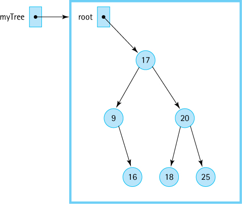
Figure 7.12 Tracing the contains operation
Here we trace this operation using the tree in Figure 7.12. In our trace we substitute actual arguments for the method parameters. It is assumed we can work with integers and are using their natural order. We want to search for the element with the key 18 in a tree myTree, so the call to the public method is
myTree.contains(18);
The contains method, in turn, immediately calls the recursive method:
return recContains(18, root);
Because root is not null and 18 > node.getInfo()—that is, 18 is greater than 17— the third if clause is executed and the method issues the recursive call:
return recContains(18, node.getRight());
Now node references the node whose key is 20, so because 18 < node.getInfo() the next recursive call is
return recContains(18, node.getLeft());
Now node references the node with the key 18, so processing falls through to the last else statement:
return true;
This halts the recursive descent, and the value true is passed back up the line of recursive calls until it is returned to the original contains method and then to the client program.
Next, we look at an example where the key is not found in the tree. We want to find the element with the key 7. The public method call is
myTree.contains(7);
followed immediately by
recContains(7, root)
Because node is not null and 7 < node.getInfo(), the first recursive call is
recContains(7, node.getLeft())
Now node is pointing to the node that contains 9. The second recursive call is issued
recContains(7, node.getLeft())
Now node is null, and the return value of false makes its way back to the original caller.
The get method is very similar to the contains operation. For both contains and get the tree is searched recursively to locate the tree element that matches the target element. However, there is one difference. Instead of returning a boolean value, a reference to the tree element that matches target is returned. Recall that the actual tree element is the info of the tree node; thus, a reference to the info object is returned. If the target is not in the tree null is returned.
public T get(T target)
// Returns info i from node of this BST where comp.compare(target, i) == 0;
// if no such node exists, returns null.
{
  return recGet(target, root);
}

private T recGet(T target, BSTNode<T> node)
// Returns info i from the subtree rooted at node such that
// comp.compare(target, i) == 0; if no such info exists, returns null.
{
  if (node == null)
    return null;             // target is not found
  else if (comp.compare(target, node.getInfo()) < 0)
    return recGet(target, node.getLeft());         // get from left subtree
  else
  if (comp.compare(target, node.getInfo()) > 0)
    return recGet(target, node.getRight());        // get from right subtree
  else
    return node.getInfo();  // target is found
}
The Traversals
The BSTExample.java application at the end of Section 7.3, “The Binary Search Tree Interface,” demonstrated our Binary Search Tree ADTs support for tree traversal. You may want to review that code and its output before continuing here.
Let us review our traversal definitions:
Preorder traversal. Visit the root, visit the left subtree, visit the right subtree.
Inorder traversal. Visit the left subtree, visit the root, visit the right subtree.
Postorder traversal. Visit the left subtree, visit the right subtree, visit the root.
Recall that the name given to each traversal specifies where the root itself is processed in relation to its subtrees.
Our Binary Search Tree ADT supports all three traversal orders through its getIterator method. As we saw in the BSTExample.java application, the client program passes getIterator an argument indicating which of the three traversal orders it wants. The getIterator method then creates the appropriate iterator and returns it. The returned iterator represents a snapshot of the tree at the time getIterator is invoked. The getIterator method accomplishes this by traversing the tree in the desired order, and as it visits each node it enqueues a reference to the node’s information in a queue of T. It then creates an iterator using the anonymous inner class approach we used before for our list iterators. The instantiated iterator has access to the queue of T and uses that queue to provide its hasNext and next methods.
The generated queue is called infoQueue. It must be declared final in order to be used by the anonymous inner class—anonymous inner classes work with copies of the local variables of their surrounding methods and therefore must be assured that the original variables will not be changed. As a result, the returned iterator cannot support the remove method. Because we are creating a snapshot of the tree for iteration, the removal of nodes during a traversal is not appropriate anyway. Here is the code for getIterator:
public Iterator<T> getIterator(BSTInterface.Traversal orderType)
// Creates and returns an Iterator providing a traversal of a "snapshot"
// of the current tree in the order indicated by the argument.
// Supports Preorder, Postorder, and Inorder traversal.
{
  final LinkedQueue<T> infoQueue = new LinkedQueue<T>();
  if (orderType == BSTInterface.Traversal.Preorder)
    preOrder(root, infoQueue);
  else
  if (orderType == BSTInterface.Traversal.Inorder)
    inOrder(root, infoQueue);

  else
  if (orderType == BSTInterface.Traversal.Postorder)
    postOrder(root, infoQueue);

  return new Iterator<T>()
  {
    public boolean hasNext()
    // Returns true if iteration has more elements; otherwise returns false.
    {
      return !infoQueue.isEmpty();
    }

    public T next()
    // Returns the next element in the iteration.
    // Throws NoSuchElementException - if the iteration has no more elements
    {
      if (!hasNext())
        throw new IndexOutOfBoundsException("illegal invocation of next "
                                     + " in BinarySearchTree iterator.
");
      return infoQueue.dequeue();
    }

    public void remove()
    // Throws UnsupportedOperationException.
    // Not supported. Removal from snapshot iteration is meaningless.
    {
      throw new UnsupportedOperationException("Unsupported remove attempted "
                                        + "on BinarySearchTree iterator.
");
    }
  };
}
As you can see, the queue holding the information for the iteration is initialized by passing it, along with a reference to the root of the tree, to a private method—a separate method for each traversal type. All that is left to do is to define the three traversal methods to store the required information from the tree into the queue in the correct order.
We start with the inorder traversal. We first need to visit the root’s left subtree, which contains all the values in the tree that are smaller than or equal to the value in the root node. Then the root node is visited by enqueuing its information in our infoQueue. Finally, we visit the root’s right subtree, which contains all the values in the tree that are larger than the value in the root node (see Figure 7.13).

Figure 7.13 Visiting all the nodes in order
Let us describe this problem again, developing our algorithm as we proceed. Our method is named inOrder and is passed arguments root and infoQueue. The goal is to visit the elements in the binary search tree rooted at root inorder; that is, first visit the left subtree inorder, then visit the root, and finally visit the right subtree inorder. As we visit a tree node we want to enqueue its information into infoQueue. Visiting the subtrees inorder is accomplished with a recursive call to inOrder, passing it the root of the appropriate subtree. This works because the subtrees are also binary search trees. When inOrder finishes visiting the left subtree, we enqueue the information of the root node and then call method inOrder to visit the right subtree. What happens if a subtree is empty? In this case the incoming argument is null and the method is exited—clearly there’s no point to visiting an empty subtree. That is our base case.
private void inOrder(BSTNode<T> node, LinkedQueue<T> q)
// Enqueues the elements from the subtree rooted at node into q in inOrder.
{
  if (node != null)
  {
    inOrder(node.getLeft(), q);
    q.enqueue(node.getInfo());
    inOrder(node.getRight(), q);
  }
}
The remaining two traversals are approached in exactly the same way, except that the relative order in which they visit the root and the subtrees is changed. Recursion certainly allows for an elegant solution to the binary tree traversal problem.
private void preOrder(BSTNode<T> node, LinkedQueue<T> q)
// Enqueues the elements from the subtree rooted at node into q in preOrder.
{
  if (node != null)
  {
    q.enqueue(node.getInfo());
    preOrder(node.getLeft(), q);
    preOrder(node.getRight(), q);
  }
}

private void postOrder(BSTNode<T> node, LinkedQueue<T> q)
// Enqueues the elements from the subtree rooted at node into q in postOrder.
{
  if (node != null)
  {
    postOrder(node.getLeft(), q);
    postOrder(node.getRight(), q);
    q.enqueue(node.getInfo());
  }
}
7.7 The Implementation Level: Transformers
To complete our implementation of the Binary Search Tree ADT we need to create the transformer methods add and remove. These are the most complex operations. The reader might benefit from a review of the subsection “Transforming a Linked List” in Section 3.4, “Recursive Processing of Linked Lists,” because a similar approach is used here as was introduced in that subsection.
The add Operation
To create and maintain the information stored in a binary search tree, we must have an operation that inserts new nodes into the tree. A new node is always inserted into its appropriate position in the tree as a leaf. Figure 7.14 shows a series of insertions into a binary tree.
For the implementation we use the same pattern that we used for contains and get. A public method, add, is passed the element for insertion. The add method invokes the recursive method, recAdd, and passes it the element plus a reference to the root of the tree. The CollectionInterface requires that our add method return a boolean indicating success or failure. Given that our tree is unbounded the add method simply returns true—it is always successful.

Figure 7.14 Insertions into a binary search tree
public boolean add (T element)
// Adds element to this BST. The tree retains its BST property.
{
  root = recAdd(element, root);
  return true;
}
The call to recAdd returns a BSTNode. It returns a reference to the new tree—that is, to the tree that now includes element. The statement
root = recAdd(element, root);
can be interpreted as “Set the reference of the root of this tree to the root of the tree that is generated when the element is added to this tree.” At first glance this might seem inefficient or redundant. We always perform insertions as leaves, so why do we have to change the root of the tree? Look again at the sequence of insertions in Figure 7.14. Do any of the insertions affect the value of the root of the tree? Yes, the original insertion into the empty tree changes the value held in the root. In the case of all the other insertions, the statement in the add method just copies the current value of the root onto itself; however, we still need the assignment statement to handle the special case of insertion into an empty tree. When does the assignment statement occur? After all the recursive calls to recAdd have been processed and have returned.
Before beginning the development of recAdd, we reiterate that every node in a binary search tree is the root node of a binary search tree. In Figure 7.15a we want to insert a node with the key value 13 into our tree whose root is the node containing 7. Because 13 is greater than 7, the new node belongs in the root node’s right subtree. We have defined a smaller version of our original problem—insert a node with the key value 13 into the tree whose root is root.right. Note that to make this example easier to follow, in both the figure and the discussion here, we use the actual arguments rather than the formal parameters, so we use “13” rather than “element” and “root.right” rather than “node.getRight()“—”root.right” is a shorthand way of writing “the right attribute of the BSTNode object referenced by the root variable.”
We have a method to insert elements into a binary search tree: recAdd. The recAdd method is called recursively:
root.right = recAdd(13, root.right);
Of course, recAdd still returns a reference to a BSTNode; it is the same recAdd method that was originally called from add, so it must behave in the same way. The above statement says “Set the reference of the right subtree of the tree to the root of the tree that is generated when 13 is inserted into the right subtree of the tree.” See Figure 7.15b. Once again, the actual assignment statement does not occur until after the remaining recursive calls to recAdd have finished processing and have returned.
The latest invocation of the recAdd method begins its execution, looking for the place to insert 13 in the tree whose root is the node with the key value 15. The method compares 13 to the key of the root node; 13 is less than 15, so the new element belongs in the tree’s left subtree. Again, we have obtained a smaller version of the problem—insert a node with the key value 13 into the tree whose root is root.right.left; that is, the subtree rooted at 10 (Figure 7.15c). Again recAdd is invoked to perform this task.

Figure 7.15 The recursive add operation
Where does it all end? There must be a base case, in which space for the new element is allocated and 13 copied into it. This case occurs when the subtree being searched is null—that is, when the subtree we wish to insert into is empty. (Remember, 13 will be added as a leaf node.) Figure 7.15d illustrates the base case. We create the new node and return a reference to it to the most recent invocation of recAdd, where the reference is assigned to the right link of the node containing 10 (see Figure 7.15e). That invocation of recAdd is then finished; it returns a reference to its subtree to the previous invocation (see Figure 7.15f), where the reference is assigned to the left link of the node containing 15. This process continues until a reference to the entire tree is returned to the original add method, which assigns it to root, as shown in Figure 7.15g and h.
While backing out of the recursive calls, the only assignment statement that actually changes a value is the one at the deepest nested level; it changes the right subtree of the node containing 10 from null to a reference to the new node containing 13. All of the other assignment statements simply assign a reference to the variable that held that reference previously. This is a typical recursive approach. We do not know ahead of time at which level the crucial assignment takes place, so we perform the assignment at every level.
The recursive method for insertion into a binary search tree is summarized as follows:
Here is the code that implements this recursive algorithm:
private BSTNode<T> recAdd(T element, BSTNode<T> node)
// Adds element to tree rooted at node; tree retains its BST property.
{
  if (node == null)
    // Addition place found
    node = new BSTNode<T>(element);
  else if (comp.compare(element, node.getInfo()) <= 0)
    node.setLeft(recAdd(element, node.getLeft()));   // Add in left subtree

  else
    node.setRight(recAdd(element, node.getRight())); // Add in right subtree
  return node;
}
The remove Operation
The remove operation is the most complicated of the binary search tree operations and one of the most complex operations considered in this text. We must ensure that when we remove an element from the tree, the binary search tree property is maintained.
The setup of the remove operation is the same as that of the add operation. The private recRemove method is invoked by the public remove method with arguments equal to the target element to be removed and the subtree to remove it from. The recursive method returns a reference to the revised tree, just as it did for add. Here is the code for remove:
public boolean remove (T target)
// Removes a node with info i from tree such that comp.compare(target,i) == 0
// and returns true; if no such node exists, returns false.
{
  root = recRemove(target, root);
  return found;
}
As with our recursive add approach, in most cases the root of the tree is not affected by the recRemove call, in which case the assignment statement is somewhat superfluous, as it is reassigning the current value of root to itself. If the node being removed happens to be the root node, however, then this assignment statement is crucial. The remove method returns the boolean value stored in found, indicating the result of the removal. The recRemove method sets the value of found to indicate whether the element was found in the tree. Obviously, if the element is not originally in the tree, then it cannot be removed.
The recRemove method receives a target and a reference to a tree node (essentially a reference to a subtree), finds and removes a node matching the target’s key from the subtree if possible, and returns a reference to the newly created subtree. We know how to determine whether the target is in the subtree; we did it for get. As with that operation, the recursive calls to recRemove progressively decrease the size of the subtree where the target node could be, until the node is located or it is determined that the node is not in the tree.
If located, we must remove the node and return a reference to the new subtree—this is somewhat complicated. This task varies according to the position of the target node in the tree. Obviously, it is simpler to remove a leaf node than to remove a nonleaf node. In fact, we can break down the removal operation into three cases, depending on the number of children linked to the node being removed:
Removing a leaf (no children). As shown in Figure 7.16, removing a leaf is simply a matter of setting the appropriate link of its parent to null.

Figure 7.16 Removing a leaf node

Figure 7.17 Removing a node with one child
Removing a node with only one child. The simple solution for removing a leaf does not suffice for removing a node with a child, because we do not want to lose all of its descendants in the tree. We want to make the reference from the parent skip over the removed node and point instead to the child of the node being removed (see Figure 7.17).
Removing a node with two children. This case is the most complicated because we cannot make the parent of the removed node point to both of the removed node’s children. The tree must remain a binary tree and the search property must remain intact. There are several ways to accomplish this removal. The method we use does not remove the node but rather replaces its
infowith theinfofrom another node in the tree so that the search property is retained. Then this other node is removed. Hmmm. That also sounds like a candidate for recursion. Let us see how this turns out.
Which tree element can be used to replace target so that the search property is retained? There are two choices: the elements whose keys immediately precede or follow the key of target—that is, the logical predecessor or successor of target. We elect to replace the info of the node being removed with the info of its logical predecessor—the node whose key is closest in value to, but less than or equal to, the key of the node to be removed.
Look back at Figure 7.14j and locate the logical predecessor of the interior nodes 5, 9, and 7. Do you see the pattern? The logical predecessor of the root node 5 is the leaf node 5, the largest value in the root’s left subtree. The logical predecessor of 9 is 8, the largest value in 9’s left subtree. The logical predecessor of 7 is 6, the largest value in 7’s left subtree. The replacement value is always in a node with either zero or one child. After copying the replacement value, it is easy to remove the node that the replacement value was in by changing one of its parent’s references (see Figure 7.18).
Examples of all three types of removals are shown in Figure 7.19.
It is clear that the removal task involves changing the reference from the parent node to the node to be removed. That explains why the recRemove method must return a reference to a BSTNode. Here we look at each of the three cases in terms of our implementation.

Figure 7.18 Removing a node with two children

Figure 7.19 Removals from a binary search tree
If both child references of the node to be removed are null, the node is a leaf and we just return null. The previous reference to this leaf node is replaced by null in the calling method, effectively removing the leaf node from the tree.
If one child reference is null, we return the other child reference. The previous reference to this node is replaced by a reference to the node’s only child, effectively jumping over the node and removing it from the tree (similar to the way we removed a node from a singly linked list).
If neither child reference is null, we replace the info of the node with the info of the node’s logical predecessor and remove the node containing the predecessor. The node containing the predecessor came from the left subtree of the current node, so we remove it from that subtree. We then return the original reference to the node (we have not created a new node with a new reference; we have just changed the node’s info reference).
Let us summarize all of this in algorithmic form as removeNode. Within the algorithm and the code, the reference to the node to be removed is node.
Now we can write the recursive definition and code for recRemove.
private BSTNode<T> recRemove(T target, BSTNode<T> node)
// Removes element with info i from tree rooted at node such that
// comp.compare(target, i) == 0 and returns true;
// if no such node exists, returns false.
{
  if (node == null)
    found = false;
  else if (comp.compare(target, node.getInfo()) < 0)
    node.setLeft(recRemove(target, node.getLeft()));
  else if (comp.compare(target, node.getInfo()) > 0)
    node.setRight(recRemove(target, node.getRight()));
  else

  {
    node = removeNode(node);
    found = true;
  }
  return node;
}
Before we code removeNode, we look at its algorithm again. We can eliminate one of the tests by noticing that the action taken when the left child reference is null also takes care of the case in which both child references are null. When the left child reference is null, the right child reference is returned. If the right child reference is also null, then null is returned, which is what we want if both nodes are null.
Here we write the code for removeNode using getPredecessor as the name of an operation that returns the info reference of the predecessor of the node with two children.
private BSTNode<T> removeNode(BSTNode<T> node)
// Removes the information at node from the tree.
{
  T data;
  if (node.getLeft() == null)
    return node.getRight();
  else if (node.getRight() == null)
    return node.getLeft();
  else
  {
    data = getPredecessor(node.getLeft());
    node.setInfo(data);
    node.setLeft(recRemove(data, node.getLeft()));
    return node;
  }
}
Now we must look at the operation for finding the logical predecessor. The logical predecessor is the maximum value in node’s left subtree. Where is this value? The maximum value in a binary search tree is in its rightmost node. Therefore, starting from the root of node’s left subtree, just keep moving right until the right child is null. When this occurs, return the info reference of that node. There is no reason to look for the predecessor recursively in this case. A simple iteration moving as far rightward down the tree as possible suffices.
private T getPredecessor(BSTNode<T> subtree)
// Returns the information held in the rightmost node of subtree
{
  BSTNode<T> temp = subtree;

  while (temp.getRight() != null)
    temp = temp.getRight();
  return temp.getInfo();
}
That is it. We used four methods to implement the binary search tree’s remove operation! Note that we use both types of recursion in our solution: direct recursion (recRemove invokes itself) and indirect recursion (recRemove invokes removeNode, which in turn may invoke recRemove). Due to the nature of our approach, we are guaranteed to never go deeper than one level of recursion in this latter case. Whenever removeNode invokes recRemove, it passes a target element and a reference to a subtree such that the target matches the largest element in the subtree. Therefore, the element matches the rightmost element of the subtree, which does not have a right child. This situation is one of the base cases for the recRemove method, so the recursion stops there.
If duplicate copies of the largest element in the subtree are present, the code will stop at the first one it finds—the one closest to the root of the tree. The remaining duplicates must be in that element’s left subtree, based on the way we defined binary search trees and the way we implemented the add method. Thus, even in this case, the indirect recursion does not proceed deeper than one level of recursion.
7.8 Binary Search Tree Performance
A binary search tree is an appropriate structure for many of the same applications discussed previously in conjunction with other collection structures, especially those providing sorted lists. The special advantage of using a binary search tree is that it facilitates searching while conferring the benefits of linking the elements. It provides the best features of both the sorted array-based list and the linked list. Similar to a sorted array-based list, it can be searched quickly, using a binary search. Similar to a linked list, it allows insertions and removals without having to move large amounts of data. Thus, a binary search tree is particularly well suited for applications in which processing time must be minimized.
As usual, there is a trade-off. The binary search tree, with its extra reference in each node, takes up more memory space than a singly linked list. In addition, the algorithms for manipulating the tree are somewhat more complicated. If all of a list’s uses involve sequential rather than random processing of the elements, a tree may not be the best choice.
Text Analysis Experiment Revisited
Let us return to the text analysis project introduced in Chapter 5, the Vocabulary Density project, and see how our binary search tree compares to the array-based and sorted array-based list approaches presented previously. Because the text analysis statistics remain unchanged we do not repeat them here—see Table 5.1 for that information. Here we concentrate solely on the execution time using three structures: an array. a sorted array, and a binary search tree. Results of the updated experiment are shown in Table 7.2.
Table 7.2 Results of Vocabulary Density Experiment
| Source | File Size | Array | Sorted Array | Binary Search Tree |
|---|---|---|---|---|
| Shakespeare’s18th Sonnet | 1 KB | 20 msecs | 23 msecs | 22 msecs |
| Shakespeare’s Hamlet | 177 KB | 236 msecs | 128 msecs | 127 msecs |
| Linux Word File | 400 KB | 9,100 msecs | 182 msecs | Stack overflow error, 33,760 msecs with revision |
| Melville’s Moby-Dick | 1,227 KB | 2,278 msecs or 2.3 seconds | 382 msecs | 334 msecs |
| Complete Works of William Shakespeare | 5,542 KB | 9.7 seconds | 1.2 seconds | 0.9 seconds |
| Webster's Unabridged Dictionary | 28,278 KB | 4.7 minutes | 9.5 seconds | 4.2 seconds |
| 11th Edition of the Encyclopaedia Britannica | 291,644 KB | 56.4 minutes | 2.5 minutes | 41.8 seconds |
| Mashup | 608,274 KB | 10 hours | 7.2 minutes | 1.7 minutes |
As you can see, the binary search tree outperforms the other two approaches in most cases, especially as the size of the files increase. In the case of the largest file, the Mashup file, analysis using the binary search tree requires only 24% of the time needed by the sorted array approach and only 0.3% of the time needed by the unsorted array approach. This is a good result and shows that when dealing with large amounts of data that need to be stored and retrieved, the binary search tree approach is a good option.
A study of the table reveals that the performance gains from the binary search tree are only clearly evident as the size of the file increases. This is because the extra overhead associated with this approach, creating nodes, managing multiple references, and the like, counterbalance the benefits of the approach when applied to smaller data sets.
The table also reveals a serious issue when the binary search tree structure is used for the Linux Word file. The application bombs—it stops executing (about 70% of the way through the data on the author’s computer) and reports a “Stack overflow error.” The error is generated because the height of the underlying tree becomes so large that the system cannot support the recursive operations add and size. The author recoded these methods to be nonrecursive so that the experiment could be concluded. Now the application completes successfully, but the amount of time required, 34 seconds, is much longer than either of the other two approaches. The problem, as you may have surmised, is that the underlying tree is completely skewed.
Insertion Order and Tree Shape
Due to the way binary search trees are constructed, the order in which nodes are inserted determines the shape of the tree. Figure 7.20 illustrates how the same data, inserted in different orders, produces very differently shaped trees.
If the values are inserted in order (or in reverse order), the tree is completely skewed (a long, “narrow” tree shape). This was the case with the Linux Word file—it is an alphabetically ordered list of words. The resulting tree has a depth of more than 45,000 nodes and is essentially a linked list of right child connections. No wonder the space allocated by the system for the method call-return stack is consumed when a recursive implementation is used.

Figure 7.20 The insertion order determines the shape of the tree
Insertion of a random mix of the elements produces a shorter, bushy tree. Because the height of the tree determines the maximum number of comparisons during a search, the tree’s shape is very important. Obviously, minimizing the height of the tree maximizes the efficiency of the search. Algorithms have been developed that adjust a tree to make its shape more desirable; some of these are discussed below; others in Section 7.10, “Tree Variations.”
Balancing a Binary Search Tree
A beneficial enhancement to our Binary Search Tree ADT operations is a balance operation that balances the tree. When a binary search tree is balanced it provides O(log2N) search, addition, and removal. The specification of the operation is
public balance();
// Restructures this BST to be optimally balanced
There are several ways to restructure a binary search tree. Our approach is simple: traverse the tree, saving the information in an array,3 and then traverse the array, saving the information back into the tree. The structure of the new tree depends on the order in which we save the information into the array and the order in which we access the array to insert the information back into the tree.
First traverse the tree inorder and insert the elements into the array. We end up with a sorted array. Next, to ensure a balanced tree we even out, as much as possible, the number of descendants in each node’s left and right subtrees. Insert elements “root first,” which means first insert the “middle” element. (If we list the elements from smallest to largest, the “middle” element is the one in the middle of the list—it has as many elements less than or equal to it as it has greater than it, or at least as close as possible.) The middle element becomes the root of the tree. It has about the same number of descendants in its left subtree as it has in its right subtree. Good. Which element do we insert next? We will work on the left subtree. Its root should be the “middle” element of all the elements that are less than or equal to the root. That element is inserted next. Now, when the remaining elements that are less than or equal to the root are inserted, about half of them will be in the left subtree of the element, and about half will be in its right subtree. Sounds recursive, does it not?
Here is an algorithm for balancing a tree based on the approach described above. The algorithm consists of two parts: one iterative and one recursive. The iterative part, Balance, creates the array and invokes the recursive part, InsertTree, which then rebuilds the tree.
As planned we first store the nodes of the tree into our array using an inorder traversal (the default traversal), so they are stored, in order, from smallest to largest. The algorithm continues by invoking the recursive algorithm InsertTree, passing it the bounds of the array. The InsertTree algorithm checks the array bounds it is passed. If the low and high bounds are the same (base case 1), it inserts the corresponding array element into the tree. If the bounds differ by only one location (base case 2), the algorithm inserts both elements into the tree. Otherwise, it computes the “middle” element of the subarray, inserts it into the tree, and then makes two recursive calls to itself: one to process the elements less than the middle element and one to process the elements greater than the middle element.
Trace the InsertTree algorithm using sorted arrays of both even and odd length to convince yourself that it works. The code for balance and a helper method insertTree follows directly from the algorithm; writing it is left for you as an exercise. Figure 7.21 shows the results of using this approach on a sample tree.
It is up to the client program to use the balance method appropriately. It should not be invoked too often, as it also has an execution cost associated with it. It is possible to provide a method that returns an indication of how balanced, or imbalanced, a tree is—which can then be used by a client to determine when to invoke balance. But testing for how balanced a tree is also has a cost. We ask you to investigate these ideas in Exercises 48 and 49.

Figure 7.21 An optimal transformation
Another, and perhaps better, approach to the issue of imbalance is to implement a more complex add operation, one that maintains a balanced tree as elements are being included. Imbalance can also be created by repeated removal of nodes so a corresponding remove method, that also maintains balance, would also need to be created. Search trees using this approach are discussed in Section 7.10, “Tree Variations.”
7.9 Application: Word Frequency Counter
We have already established that our binary search tree is a good structure to use when analyzing text files, at least normal text files—that is, files representing novels, technical manuals, and news stories—we just do not want to use it without some sort of balancing strategy with files like the Linux Word file. In this section we develop a word frequency counter that uses our binary search tree. The application is to read a text file and generate an alphabetical listing of the unique words that the file contains, along with a count of how many times each word occurs.
To allow users to control the amount of useful output from the generator, based on the particular problem they are studying, the generator must allow users to specify a minimum word size and a minimum frequency count. The generator should skip over words smaller than the minimum word size; it should not include a word on its output list if the word occurs fewer times than the minimum frequency count. Finally, the generator should present a few summary statistics: the total number of words, the number of words whose length is at least the minimum word size, and the number of unique words of at least the specified size whose frequency is at least the minimum frequency count.
The WordFreq Class
To associate a count with each unique word from the file we create a class called WordFreq to hold a word frequency pair. A quick analysis tells us that we have to be able to initialize objects of the class, increment the frequency, and observe both the word and the frequency values.
The code for the WordFreq class is very straightforward. It is placed in the support package. A few observations are appropriate:
The constructor initializes the
freqvariable to 0. As a consequence, the main program must increment aWordFreqobject before placing it on the tree for the first time. We could have coded the constructor to set the original frequency to 1, but it is more natural to begin a frequency count at 0. There may be other applications that can useWordFreqwhere this feature would be important.In the
toStringmethod, we use Java’sDecimalFormatclass to force the string generated from the frequency count to be at least five characters wide. This helps line up output information for applications such as our word frequency generator.
//---------------------------------------------------------------------------
// WordFreq.java              by Dale/Joyce/Weems                   Chapter 7
//
// Defines word-frequency pairs
//---------------------------------------------------------------------------
package support;

import java.text.DecimalFormat;

public class WordFreq implements Comparable<WordFreq>
{
  private String word;
  private int freq;

  DecimalFormat fmt = new DecimalFormat("00000");

  public WordFreq(String newWord)
  {
    word = newWord;
    freq = 0;
   }

  public String getWordIs(){return word;}
  public int getFreq(){return freq;}

  public void inc()
  {
    freq++;
  }

  public int compareTo(WordFreq other)
  {
    return this.word.compareTo(other.word);
  }

  public String toString()
  {
    return(fmt.format(freq) + " " + word);
  }
}
The Application
Our approach for this application borrows quite a bit from the VocabularyDensity application developed in Chapter 5 and revisited in the previous section. The application scans the input file for words, and after reading a word, it checks to see if a match is already in the tree, and if not it insets the word. What is actually inserted is a WordFreq object that holds the word and a frequency count of 1.
Unlike the VocabularyDensity application, however, there is processing to attend to even if the word is already in the tree. In that case the application must increment the frequency associated with the word. It needs to get the corresponding WordFreq object from the tree, increment its count, and then add it back into the tree. But wait—if the application gets the object from the tree and then adds it back, there will be two copies of it in the tree. So it also needs to remove the object from the tree before processing it. If the word is not already in the tree it needs to insert it with a corresponding count of 1. The following algorithm summarizes this discussion. Assume that wordFromTree and wordToTry are WordFreq objects and that the latter contains the next word from the input file that is at least the minimum word size in length.
The first thing we notice is the repeated access to the tree required for each word. Potentially the application may have to check the tree to see whether the word is already there, get the word from the tree, remove the word from the tree, and save the word back into the tree. This is not good. Our input files could have tens of thousands of words, so even though the binary search tree provides an efficient structuring mechanism, it is not a good idea to access it so many times for each word. Can we do better?
Recall that our tree stores objects “by reference.” When a WordFreq object is retrieved from the tree, it is actually a reference to the object that is retrieved. If that reference is used to access the object and increment its frequency count, the frequency count of the object in the tree is incremented. It is not necessary to remove the word from the tree and then add it back.
In our discussion of the perils of “store by reference” in the feature “Implementing ADTs ‘by Copy’ or ‘by Reference’” found in Section 5.5, “Sorted Array-Based Collection Implementation,” we stated that it is dangerous for the client to use a reference to reach into a data structure hidden by an ADT and change a data element. But as we also noted, this practice is dangerous only if the change affects the parts of the element used to determine the underlying organization of the structure. In this case, the structure is based on the word information of a WordFreq object; the application is changing the frequency information. It can reach into the tree and increment the frequency count of one of the tree’s elements without affecting the tree’s structure. We change the name of our variable to reflect the fact that the object is still in the tree. We can reduce our algorithm to:
That is a significant improvement, but we can still do better. Do you see how? Instead of using contains to determine if the word is already in the tree we can use get. If get returns a null, then the word is not in the tree. If get returns a non-null, then the word is in the tree. Using this approach we reduce the number of accesses of the tree as we no longer need to execute both contains and get:
Overall, we have reduced the maximum number of times the tree is “searched” to handle a matched word from 4 to 1. Much better.
Figure 7.22 displays a trace of this algorithm, showing the changes that occur to the variables when “aardvark” is the next “word to try” and assuming that “aardvark” has already been processed five times, as well as “fox” (three times) and “zebra” (seven times). Part (a) of the figure shows the status before processing. Note that wordInTree is null at this point. Part (b) shows the status after the step
wordInTree = tree.get(wordToTry)
As you can see, wordInTree now holds a reference into the tree. Because the boolean expression (wordInTree != null) evaluates to true, the next statement executed is
wordInTree.inc()
that increments the frequency of the WordFreq object within the tree (as shown in part (c) of the figure).
The remainder of the application is straightforward. Based on the user input we do need to filter the words under consideration by word size and filter the output by word count. These requirements are both handled easily with simple if statements. The application is below.
//---------------------------------------------------------------------------
// WordFreqCounter.java         by Dale/Joyce/Weems                 Chapter 7
//
// Displays a word frequency list of the words listed in the input file.
// Prompts user for minSize and minFreq.
// Does not process words less than minSize in length.
// Does not output words unless their frequency is at least minFreq.
//---------------------------------------------------------------------------
package ch07.apps;

Figure 7.22 Trace of “Handle the Next Word 3” algorithm
import java.io.*;
import java.util.Scanner;
import ch07.trees.*;
import support.WordFreq;

public class WordFreqCounter
{
  public static void main(String[] args) throws IOException
  {
    String word;
    WordFreq wordToTry;
    WordFreq wordInTree;

    BinarySearchTree<WordFreq> tree = new BinarySearchTree<WordFreq>();

    int numWords = 0;
    int numValidWords = 0;

    int numValidFreqs = 0;
    int minSize;
    int minFreq;
    int treeSize;

    // Set up command line reading
    Scanner scan = new Scanner(System.in);

    // Set up file reading
    String fn;
    System.out.print("File name > ");
    fn = scan.next();
    Scanner wordsIn = new Scanner(new FileReader(fn));
    wordsIn.useDelimiter("[^a-zA-Z']");  // delimiters are nonletters,'

    // Get word and frequency limits from user
    System.out.print("Minimum word size> ");
    minSize = scan.nextInt();
    System.out.print("Minimum word frequency> ");
    minFreq = scan.nextInt();

    // Process file
    while (wordsIn.hasNext())      // while more words to process
    {
      word = wordsIn.next();
      numWords++;
      if (word.length() >= minSize)
      {
        numValidWords++;
        word = word.toLowerCase();
        wordToTry = new WordFreq(word);
        wordInTree = tree.get(wordToTry);
        if (wordInTree != null)
        {
          // word already in tree, just increment frequency
          wordInTree.inc();
        }
        else
        {
          // insert new word into tree
          wordToTry.inc();               // set frequency to 1
          tree.add(wordToTry);
        }
      }
    }

    // Display results
    System.out.println("The words of length " + minSize + " and above,");
    System.out.println("with frequency counts " + minFreq + " and above:");
    System.out.println();
    System.out.println("Freq  Word");
    System.out.println("----- -----------------");
    for (WordFreq wordFromTree: tree)
    {
      if (wordFromTree.getFreq() >= minFreq)
      {
        numValidFreqs++;
        System.out.println(wordFromTree);
      }
    }
    System.out.println();
    System.out.println(numWords + " words in the input file.  ");
    System.out.println(numValidWords + " of them are at least " + minSize
                       + " characters.");
    System.out.println(numValidFreqs + " of these occur at least "
                       + minFreq + " times.");
    System.out.println("Program completed.");
  }
}
Here we show the results of running the program on a text file containing the complete works of William Shakespeare. The minimum word size was set to 10 and the minimum frequency count was set to 100. Ten words meeting those criteria were found. This application is a useful text analysis tool—and it is fun, too. What is a “bolingbroke”?4
File name > input/literature/shakespeare.txt
Minimum word size> 10
Minimum word frequency> 100
The words of length 10 and above,
with frequency counts of 100 and above:

Freq  Word
----- -----------------
00219 antipholus
00141 attendants

00175 bolingbroke
00254 buckingham
00120 conscience
00213 coriolanus
00572 gloucester
00102 honourable
00148 northumberland
00159 themselves

1726174 words in the input file.
15828 of them are at least 10 characters.
10 of these occur at least 100 times.
Program completed.
7.10 Tree Variations
Our goal in the Variations sections of this text is to instruct the reader about alternate definitions and implementation approaches for each of the ADTs studied. We also hope to arouse the reader’s curiosity about the variety of data structures that exist and show that the possibilities are “unbounded” when it comes to defining new ways to structure our data. Nowhere is this more evident than with the Tree ADT, for which more variations may exist than for all the other ADTs considered together. Trees can be binary, trinary (up to three children per node), n-ary (up to n children per node), alternatingary, balanced, not balanced, partially balanced, self-adjusting, and store information in their nodes or their edges or both. With trees, even the variations have variations!
Application-Specific Variations
Given the wide variety of trees it is difficult (but not impossible) to define a general tree ADT. The Java Library does not include a general tree structure and neither do most textbooks. Often with trees we let the specific target application dictate the definition, assumptions, rules, and operations associated with a specific implementation. Here we review some of the popular specific uses for trees.
Decision Trees
What to do today? The answer to this question might depend on the sequence of answers to a host of other questions: is my schoolwork up-to-date, how is the weather, what is my bank account balance? When we work through a series of questions and our answers lead to other questions, yet ultimately to a solution, we are traversing a decision tree.

Support for creating and using such trees is often included in business management tools. These trees can consist of separate types of nodes such as boolean question nodes, multiple choice question nodes, chance nodes, and answer nodes. Static decision trees can be implemented using nested if-else and switch statements, whereas dynamic ones would require implementations similar to those we presented in this chapter.
Expression/Parse Trees

Arithmetic expressions can be ambiguous. For example, the expression 5 + 3 × 2 might evaluate to 16 or 11 depending on the order in which you perform the operations. We resolve this ambiguity by creating rules for order of evaluation or by using grouping symbols, such as parenthesis. Another way to solve the problem is to store the expression in a tree. A tree node that holds an operation indicates that the operation is to be performed on its children. There is no ambiguity. Specially designed tree traversals are used to evaluate the expression.
In addition to storing and helping us evaluate an expression in an unambiguous manner, expression trees can be used to translate expressions from one form to another. Looking at the tree on the right above we “see” the infix expression (5 + 3) × 2. But consider the result of a postorder traversal: 5 3 + 2 }. You might recognize that as the postfix expression that corresponds to the given infix expression. Similarly, we can generate “prefix” expressions using a preorder traversal.
Expressions trees can be binary or n-ary. Arithmetic expression trees are a specific form of a more general type of tree, a parse tree. Formal language definition relies on a sequence of expressions describing how strings may be combined into legal sentences. These expressions follow the same rules as arithmetic expressions and can, therefore, also be stored as trees. So expression trees, or parse trees as they are usually called, can be used to store a legal sentence of a formal grammar. Since programming languages are formal languages, a parse tree can be used to store an entire computer program!
R-Trees

R-Trees (Rectangle Trees) and their variants deal with storing hierarchical spatial data and can be used in search and navigational systems. Desks sit within a classroom, classrooms line a hallway, hallways are on floors, floors are in wings, wings are in buildings, buildings are on campuses, and so on. R-trees can be used to store the relative locations of all of these things in a manner that supports efficient retrieval. Inner nodes represent bounding rectangles which contain, literally, all of their descendants. Leaf nodes represent specific objects.
R-Trees are a good example of a tree structure that was created to address a specific problem, in this case support for geo-data related applications (identify all the lakes within 40 miles of point X). Given the constraints of a particular problem, computer scientists design efficient structures to support problem solution.
Tries/Prefix Trees
A Trie is an interesting structure because the information it stores is associated with its edges. Tries are used as collections, with a goal toward making the contains operation as quick as possible. Trie is pronounced as “tree” as the name derives from the “trie” in “retrieval”.

In particular, tries are useful for storing strings, or any other information that can be broken into a sequence of atomized parts, such as binary numbers. Let us look at how a trie stores strings of characters. In the example trie shown here the root represents the empty string. As we traverse from the root to a leaf we build a string, adding the character associated with each link as we go. When we arrive at a leaf we have built one of the strings that is contained in the trie. Contained strings can also be associated with inner nodes. The shaded nodes in our sample tree all indicate strings contained in the trie.
To determine if a given string is stored in our tree we simply access the string character by character, traversing the trie as we go. If we reach a point where no traversal path is possible before we reach the end of the string then the answer is “no, the string is not stored in the trie”. If we reach the end of the string and are left in a “shaded” node within the trie then the answer is “Yes!”.
Tries are useful for word game applications, spell checkers, and hyphenators. They are especially appropriate for autocompletion of text, such as the apps that suggest what word you are typing when you are texting. Do you see why?
Balanced Search Trees
The Binary Search Tree ADT presented in this chapter is an excellent collection structure for holding “random” data, but suffers from one major weakness—it can become unbalanced. In the extreme case (see Figure 7.20c) an unbalanced binary search tree acts no differently than a linked list—essentially it is a linked list. Many search tree variations have been invented to address this weakness, each in turn with their own strengths and weaknesses. Different variations have different definitions of what it means to be balanced.
B-Trees

A B-Tree (B for “Balanced”) is a search tree that allows internal nodes to hold multiple values and have multiple children. Within a node the values and child links are stored in order, and a form of the binary search tree property is maintained in terms of the relationship between the information in child nodes and their parents.
Since a B-Tree node can contain a great deal of information, processing that information during a search or change to the tree requires more effort than processing a node of a binary search tree. B-trees were originally designed to support retrieval of information from disk storage systems and they are often used with large scale database systems. In these systems the time required to read information is the most costly part of processing. Since B-Trees store a lot of information in a “flat” tree they are perfect for such systems. A minimal number of time consuming “read from disk” operations are required to find information in the B-Tree and the extra time required for processing a node, once it has been read, is not important in the overall scheme of things.
A 2-3-4 tree can be implemented using a binary tree structure called a red-black tree. In this structure nodes are “colored” either red or black (each node must hold an extra boolean value that indicates this information). The color of a node indicates how its value fits into the corresponding 2-3-4 tree. For example, a 4-node holding the information [B, D, F] is modeled by a “black” node containing [D], with a left child “red” node containing [B] and a right child “red” node containing [F]. The rules for what constitutes a red-black tree are somewhat complicated but suffice it to say it provides all the benefits of a 2-3-4 tree plus the added benefit of only requiring a single node type, a binary tree node, to support its implementation. Although the defining rules are more complex, implementation is simpler.
Note that the Java Library does not provide a Tree ADT—but it does include two important classes that use tree implementations. The Java TreeMap class supports maps (see Chapter 8) and the Java TreeSet class supports sets (see Section 5.7, “Collection Variations”). In both cases the internal representation is a red-black tree.
AVL Trees
AVL trees were defined in a paper in 1962 written by Adeleson-Velsky and Landis. They define balance from the local perspective of a single node—in an AVL tree the difference in height between a node’s two subtrees can be at most 1. Let us call the difference in height between two subtrees of a node its “balance factor”. Returning again to Figure 7.20, the tree in part (a) of the figure is an AVL tree since the balance factor of each of its nodes is 0. The tree in part (b) of the figure is not an AVL tree because, for example, the balance factor of its root node is 3. Obviously the tree in part (c) of the figure is also not an AVL tree.
Having each node in a tree exhibit a balance factor ≤ 1 results in a relatively well-balanced tree. Searching for information in an AVL tree is an O(log2N) operation, even in the worst case. But what about addition and removal of information? During addition and removal of nodes extra work is required to ensure the tree remains balanced. Let us consider addition of a node. Figure 7.23a shows an AVL tree containing five nodes. The balance factor of its nodes, top to bottom, left to right are 1, 0, 0, 0, 0. Figure 7.23b shows the result of adding 5 to the tree. The new tree is no longer an AVL tree, since the balance factor of its nodes, top to bottom, left to right are 2, 1, 0, 1, 0, 0. Any imbalance created in an AVL tree by an addition will be along the path of nodes that were visited to determine the addition location, and in this case the imbalance is exhibited at the root node.
Temporary imbalance in an AVL tree is handled by performing one of four potential rotations. In our example the rotation known as a “right rotation” or more simply the “R rotation” is performed on the root. The tree is “rotated” with the root moving down to the right and its left child moving up to become the new root. The result of the rotation, which is accomplished with three reference assignment statements, is shown in Figure 7.23c. Depending on the nature of the imbalance other rotations might be required (L, LR, and RL rotations). All needed rotations are accomplished with a few reference assignment statements. Although in some cases multiple rotations are required to rebalance a tree, the overall cost of additions and removals is never more than O(log2N).
Research shows that AVL trees perform especially well in situations where an original tree construction includes insertions of sequences of elements “in order”, and is followed by long sequences of search operations.

Figure 7.23 Adding a node to an AVL tree
Summary
In this chapter we learned about trees and their many uses. The binary search tree may be used to structure sorted information to reduce the search time for any particular element while at the same time allowing relatively fast addition and removal of information. For applications in which direct access to the elements in a sorted structure is needed, the binary search tree is a very useful data structure. If the tree is balanced, access to any node in the tree is an O(log2N) operation. The binary search tree combines the advantages of quick random access (like a binary search on a sorted linear list) with the flexibility of a linked structure.
We also saw that the binary search tree operations could be implemented very elegantly and concisely using recursion. This makes sense, because a binary tree is itself a “recursive” structure: Any node in the tree is the root of another binary tree. Each time we moved down a level in the tree, taking either the right or left path from a node, the size of the (current) tree is reduced, a clear case of the smaller-caller. For comparison we implemented the size operation both recursively and iteratively—the iterative version made use of our Stack ADT.
The benefits of a binary search tree diminish if the tree is skewed. We discussed a tree-balancing approach that can be used to keep a binary search tree balanced, and in the Variations section we introduced the concept of self-balancing trees.
Figure 7.24 is a UML diagram showing the relationships among the classes and interfaces involved in our Binary Search Tree ADT. It shows that the BSTInterface extends both this text’s CollectionInterface and the library’s Iterable interface.

Figure 7.24 Classes and interfaces related to the Binary Search Tree ADT
Thus in addition to the min, max, and getIterator operations our binary search trees must implement all of the abstract methods found in those interfaces. Our BinarySearchTree class is the most complex class we have developed so far.
Exercises
7.1 Trees
-
For each of the following application areas state whether or not the tree data structure appears to be a good fit for use as a storage structure, and explain your answer:
chess game moves
public transportation paths
relationship among computer files and folders
genealogical information
parts of a book (chapters, sections, etc.)
programming language history
mathematical expression
-
Java classes are related in a hierarchical manner defined by inheritance; in fact we sometimes speak of the “Java Inheritance Tree.” The hierarchy within the
Java.langpackage is described here:https://docs.oracle.com/javase/8/docs/api/java/lang/package- tree.html.
Answer the following questions about that hierarchy viewed as a tree.
What is the root?
What is the height of the tree?
Which node has the most children?
How many leaves are there?
-
Following the example in Figure 7.1d, draw a tree that represents this maze:

-
Answer the questions below about the following tree, using the letters that label the nodes:

Which node is the root?
Which node is the parent of F?
Which node(s) are the children of H?
Which node(s) are the ancestors of M?
Which node(s) are the descendants of T?
Which node(s) are the siblings of S? of H?
What is the height of the tree?
In what order are the nodes visited by a breadth-first traversal?
In what order are the nodes visited by a depth-first traversal?
-
Create a table similar to Table 7.1 that shows a trace of a
Depth-First Traversal for the sample tree in Figure 7.2.
Breadth-First Traversal for the sample tree in Exercise 4.
Depth-First Traversal for the sample tree in Exercise 4.
-
Draw a tree (multiple answers might be possible) that
Has four nodes and is height 1.
Has four nodes and is height 3.
Has more nodes at level 2 than at level 1.
Has five nodes and three are leaves.
Has six nodes and two are leaves.
Has four interior nodes.
Has a breadth-first traversal of A B C D E F.
Has a depth-first traversal of A B C D E F.
Has a breadth-first traversal of A B C D E F and a depth-first traversal of A B C E F D.
-
Brainstorm: Describe two different approaches to implementing a general tree data structure.
7.2 Binary Search Trees
-
True/False. Explain your answer.
Every binary tree is a binary search tree.
Every binary search tree is a tree.
Every binary search tree is a binary tree.
A node in a binary tree must have two children.
A node in a binary tree can have more than one parent.
Each node of a binary search tree has a parent.
In a binary search tree the info in all of the nodes in the left subtree of a node are less than the info in all of the nodes in the right subtree of the node.
In a binary search tree the info in all of the nodes in the left subtree of a node are less than the info in the node.
A preorder traversal of a binary search tree processes the nodes in the tree in the exact reverse order that a postorder traversal processes them.
-
Draw a single binary tree that has both inorder traversal E B A F D G and preorder traversal A B E D F G.
-
Draw a single binary tree which has inorder traversal T M Z Q A W V and postorder traversal Z M T A W V Q.
-
Draw three binary search trees of height 2 containing the nodes A, B, C, D, and E.
-
What is the
maximum number of levels that a binary search tree with 100 nodes can have?
minimum number of levels that a binary search tree with 100 nodes can have?
maximum total number of nodes in a binary tree that has N levels? (Remember that the root is level 0.)
maximum number of nodes in the Nth level of a binary tree?
number of ancestors of a node in the Nth level of a binary search tree?
number of different binary trees that can be made from three nodes that contain the key values 1, 2, and 3?
number of different binary search trees that can be made from three nodes that contain the key values 1, 2, and 3?
-
Answer the following questions about the binary search tree with root referenced by
rootA(see below).What is the height of the tree?
Which nodes are on level 3?
Which levels have the maximum number of nodes that they could contain?
What is the maximum height of a binary search tree containing these nodes?
What is the minimum height of a binary search tree containing these nodes?
What is the order in which nodes are visited by a preorder traversal?
What is the order in which nodes are visited by an inorder traversal?
What is the order in which nodes are visited by a postorder traversal?
What is the order in which nodes are visited by a depth-first traversal?
What is the order in which nodes are visited by a breadth-first traversal?
-
Repeat the previous question but use binary search tree with root referenced by
rootB.
7.3 The Binary Search Tree Interface
-
List all the methods required by the
BSTInterfaceand classify each as observer, transformer, or both. -
In addition to the operations required by the
BSTInterface, define at least three more operations that might be useful for a Binary Search Tree ADT to provide. -
Explain the concept of a “snapshot” of a structure. Explain why it does not make sense for our binary search tree iterators to support a
removeoperation. -
For this question assume that binary search tree
treeA(with root referenced byrootAas shown above) has been declared and instantiated as an object of a class that correctly implementsBSTInterface. What is the output of each of the following code sections (these sections are independent; that is, you start over again with the tree as shown in the figure above for each section):System.out.println(treeA.isFull()); System.out.println(treeA.isEmpty()); System.out.println(treeA.size()); System.out.println(treeA.min()); System.out.println(treeA.max()); System.out.println(treeA.contains('R')); System.out.println(treeA.remove('R')); System.out.println(treeA.remove('R')); System.out.println(treeA.get('S'));Iterator<Character> iter; iter = treeA.getIterator(BSTInterface.Traversal.Preorder); while (iter.hasNext()) System.out.print(iter.next()); System.out.println(); for (Character ch: treeA) System.out.print(ch); System.out.println(); iter = treeA.iterator(); while (iter.hasNext()) System.out.print(iter.next());
Iterator<Character> iter;
iter = treeA.getIterator(BSTInterface.Traversal.Preorder);
treeA.remove('N'); treeA.remove('R');
while (iter.hasNext())
   System.out.print(iter.next());
iter = treeA.getIterator(BSTInterface.Traversal.Inorder);
while (iter.hasNext())
   System.out.print(iter.next());
-
 Using the Binary Search Tree ADT: For this question you should use the methods listed in the
 BSTInterfaceand standard Java control operations.Assume that binary search tree
wordshas been declared and it holdsStringobjects. Write a section of code that prompts the user for a sentence, and then displays the words from the sentence in alphabetical order.Assume that binary search tree
numbershas been declared and it holdsIntegerobjects. Write a section of code that generates 1,000 random numbers between 1 and 10,000 and stores them innumbers. It then generates 20 more numbers and reports for each whether or not it is contained innumbers.Assume that binary search tree
numbershas been declared and it holdsIntegerobjects. Write a section of code that generates 1,000 random numbers between 1 and 10,000 and stores them innumbers. It then outputs the average value of the numbers and how many of the numbers are less than that average.
7.4 The Implementation Level: Basics
-
Compare and contrast the
DLLNodeandBSTNodeclasses found in this text’ssupportpackage. -
Explain the difference between the two constructors of the
BinarySearchTreeclass. -
Suppose
treeis a variable of typeBinarySearchTree<String>and represents a tree containing the strings “alpha,” “beta,” “gamma,” and “zebra,” with “gamma” as the root and “beta” as one of the leaves. Draw a detailed figure that demonstrates the contents of the external variabletree, the internal variableroot, plus the contents of the fourBSTNodeobjects. -
The
FamousPersonclass is part of this text’ssupportpackage and was introduced in Section 5.4, “Comparing Objects Revisited,” and revisited in Section 6.4, “Sorted Array-Based List Implementation.” Show how you would instantiate a binary search treepeopleto holdFamousPersonobjects ordered byLast name, First name
Year of birth
-
Which method of the
BinarySearchTreeclass is more efficient,maxormin? Explain your answer. -
For each of the following trees, state how many times the body of the while loops of the
minandmaxmethods of theBinarySearchTreeclass would be executed, if the methods are invoked on:an empty tree
a tree consisting of a single node
the tree in Figure 7.20a
the tree in Figure 7.20b
the tree in Figure 7.20c
-
Suppose
numbersis a variable of classBinarySearchTree<Integer>andvalueis a variable of typeint. Write a Java statement that printstrueifvalueis in-between the largest and smallest values stored innumbers, andfalseotherwise.
7.5 Iterative Versus Recursive Method Implementations
-
Compare and contrast the approach we used for the
sizemethod when implementing our List ADT for theLBListclass in Chapter 6 (maintain an instance variable representing size) to the approach used for theBinarySearchTreeclass (calculate the size when asked). -
Use the Three-Question Method to verify the recursive version of the
sizemethod. -
 Design and implement a method
 min2forBinarySearchTree, functionally equivalent to theminmethod, which uses recursion. -
Design and implement a method
leafCountforBinarySearchTreethat returns the number of leaves in the tree anduses recursion.
does not use recursion.
-
Design and implement a method
oneChildforBinarySearchTreethat returns the number of nodes in the tree that have exactly one child anduses recursion.
does not use recursion.
-
Design and implement a method
heightforBinarySearchTree, that returns the height of the tree anduses recursion.
does not use recursion.
7.6 The Implementation Level: Remaining Observers
-
For each of the following trees state how many times the
getLeft,getRight, andgetInfomethods are invoked if thecontainsmethod of theBinarySearchTreeclass is called with an argument of D on:an empty tree
a tree consisting of a single node that contains D
a tree consisting of a single node that contains A
a tree consisting of a single node that contains E
the tree in Figure 7.20a
the tree in Figure 7.20b
the tree in Figure 7.20c
-
What would be the effect of changing the first < comparison to <= in the
recContainsmethod of the BinarySearchTree class? -
Design and implement a method
contains2forBinarySearchTree, functionally equivalent to thecontainsmethod, that does not use recursion. -
Suppose
getIteratoris invoked on the tree in Figure 7.12 and passed an argument indicating that an inorder traversal is desired. Show the sequence of ensuing method calls (you can indicate arguments using an integer that represents the info in the node) that are made to build the queue. Repeat for a postorder traversal. -
Suppose that in place of using a queue within our traversal generation code we used a stack. Instead of enqueuing and dequeuing we push and top/pop the elements, but we make no other changes to the code. What would such a change mean for
the preorder traversal
the inorder traversal
the postorder traversal
-
Enhance the Binary Search Tree ADT so that it supports a “level-order” traversal of the nodes, in addition to preorder, inorder, and postorder traversals.
7.7 The Implementation Level: Transformers
-
Show how we visualize the binary search tree with root referenced by
rootA(page 490) after each of the following changes. Also list the sequence ofBinarySearchTreemethod calls, both public and private, that would be made when executing the change. Use the original tree to answer each part of this question.Add node C.
Add node Z.
Add node Q.
Remove node M.
Remove node Q.
Remove node R.
-
Draw the binary search tree that results from starting with an empty tree and
adding 50 72 96 94 26 12 11 9 2 10 25 51 16 17 95
adding 95 17 16 51 25 10 2 9 11 12 26 94 96 72 50
adding 10 72 96 94 85 78 80 9 5 3 1 15 18 37 47
adding 50 72 96 94 26 12 11 9 2 10, then removing 2 and 94
adding 50 72 96 94 26 12 11 9 2 10, then removing 50 and 26
adding 50 72 96 94 26 12 11 9 2 10, then removing 12 and 72
-
Alternate implementations of the
addmethod:We implemented the
addmethod by invoking arecAddmethod as follows:root = recAdd(element, root);
As explained in the text, we used this approach so that in the case of adding to an empty tree we correctly reset the value in
root. An alternate approach is to first handle that special case within theaddmethod itself, before invokingrecAdd. With this new approachrecAddneed not return anything; it just handles the addition of the element. Design and implement a methodadd2forBinarySearchTree, functionally equivalent to theaddmethod, that uses this alternate approach.Design and implement a method
add3forBinarySearchTree, functionally equivalent to theaddmethod, that does not use recursion.
7.8 Binary Search Tree Performance
-
Suppose 1,000 integer elements are generated at random and are inserted into a sorted linked list and a binary search tree (BST). Compare the efficiency of searching for an element in the two structures.
-
Suppose 1,000 integer elements are inserted in order, from smallest to largest, into a sorted linked list and a binary search tree. Compare the efficiency of searching for an element in the two structures.
-
Fill in the following table with the worst case efficiency order for each of the listed operations, given the listed internal representation. Assume the collection contains N elements at the time the operation is invoked. Assume an efficient algorithm is used (as efficient as allowed by the representation). Assume the linked lists have a pointer to the “front” of the list only.
Unsorted Array Unsorted Linked List Sorted Array Sorted Linked List Skewed BST Bushy BST isEmpty min max contains add remove -
Draw the new tree that would be created by traversing the binary search tree with root referenced by
rootA(page 490) in the following order, and as the nodes are visited, adding them to the new tree:Preorder
Inorder
Postorder
Levelorder
-
Using the Balance algorithm, show the tree that would be created if the following values represented the inorder traversal of the original tree.
a. 3 6 9 15 17 19 29 b. 3 6 9 15 17 19 29 37 c. 1 2 3 3 3 3 3 3 3 24 37 -
Revise our
BSTInterfaceinterface andBinarySearchTreeclass to include thebalancemethod. How can you test your revision? -
Fullness Experiment:
Design and implement a method
heightforBinarySearchTreethat returns the height of the tree (you have already done this if you completed Exercise 32).Define the fullness ratio of a binary tree to be the ratio between its minimum height and its height (given the number of nodes in the tree). For example, the tree in Figure 7.5a has a fullness ratio of 1.00 (its minimum height is 3 and its height is 3) and the tree in Figure 7.6c has a fullness ratio of 0.33 (its minimum height is 3 and its height is 9). Implement a method
fRatioto be added to theBinarySearchTreeclass that returns the fullness ratio of the tree.Create an application that generates 10 “random” trees, each with 1,000 nodes (random integers between 1 and 3,000). For each tree output its height, optimal height, and fullness ratio.
Submit a report that includes your code for the
heightmethod, thefRatiomethod, the application code, sample output, and a short discussion. The discussion should include consideration of how thefRatiomethod might be used by an application to keep its search trees reasonably well balanced.
-
Fullness Experiment Part 2 (assumes you did the previous exercise):
Create an application that is capable of creating a “random” tree of 1,000 nodes (integers between 1 and 3,000). Each time one of the integers is generated it has a k% chance of being 42 and a (1-k)% chance of being a random integer between 1 and 3,000. For example, if k is 20 then approximately 20% of the integers in the tree will be 42 and the other 80% will be spread between 1 and 3,000. The application should output the tree’s height, optimal height, and fullness ratio. Test the application on various values of k.
Expand your application so that it generates 10 trees for each value of k varying between 10 and 90, in increments by 10. That is a total of 90 trees. For each value of k output the average tree height and fullness ratio.
Submit a report that includes your code, sample output, and a discussion. Include descriptions of situations where we might store information that is “uneven”—where certain values occur more frequently than others.
7.9 Application: Word Frequency Counter
-
List all of the classes used directly by the
WordFreqCounterapplication. -
Describe the effect that each of the following changes would have on the
WordFreqCounterapplication.Remove the call to the
useDelimitermethod of theScannerclass.Remove the call to the
toLowerCasemethod of theStringclass.Change the call to the
toLowerCasemethod to a call to thetoUpperCasemethod.In the inner if clause of the while loop, change the statement
wordInTree.inc()towordToTry.inc().
-
Create an application that will read a text file (file name/location provided through a command line argument) and display the longest word (or words if there is a tie) in the file and how many times they occur.
-
Create an application that will read a text file (file name/location provided through a command line argument) and display the most frequently used word (or words if there is a tie) in the file and how many times they occur.
-
Create an application that will read a text file (file name/location provided through a command line argument) and display the word or words in the file that occur exactly once.
-
An n-gram is a sequence of n items (numbers, characters, words) from some source. For example, the phrase “scoo be do be do be” contains the word-based 2-grams “scoo be” (once), “be do” (twice), and “do be” (twice). N-grams are used by computational linguists, biologists, and data compression experts in a multitude of ways. They can be especially useful in prediction models, where you have the start of a sequence of items and want to predict what is next—for example, when you text on your phone it might predict what word you want next as a shortcut. Write and test code that
Acts like the
WordFreqCounterapplication but instead of asking the user for the minimum word and frequency size it asks the user for a value of n and an associated minimum n-gram frequency, then tracks the frequency of n-grams from the input text, for that n.Enhance your application from part (a) so that after reporting the results for the n-grams it allows the user repeatedly to enter a group of n words and it reports back the top three most likely words that follow that group, along with the percentage of time within the text that group of words is followed by the reported word. For example, the interaction from running the application might look like this:
File name >  somefile.txt
n-gram length> 3
Minimum n-gram frequency> 40
The 3-grams with frequency counts of 40 and above:

Freq  3-gram
----------------------
00218 one of the
00105 is in the
00048 at the end

Enter 3 words (X to stop): one of the

12.7% one of the most
 8.3%    one of the first
 3.4%   one of the last

. . .
7.10 Tree Variations
-
Draw a decision tree for deciding where to eat.
-
For the following mathematical expression
(56 + 24) × 2 – (15 / 3)
draw the expression tree.
what is a preorder traversal of the tree?
postorder?
-
Draw the trie containing the following words:
dan date danger dang dog data daniel dave -
Bob decides that the efficiency of searching a B-tree is dependent on how many levels there are in the tree. He decides he will store his 1,000 elements in a B-tree which contains only one node, a root node with all 1,000 elements. Because the height of his tree is 0, he believes he will be rewarded with constant search time. What do you tell Bob?
-
In the subsection AVL Trees, we defined the “balance factor” of a node. What is the balance factor of
Node A in the tree in Figure 7.6a.
Node A in the tree in Figure 7.6b.
Node A in the tree in Figure 7.6c.
Node C in the tree in Figure 7.6a.
Node C in the tree in Figure 7.6b.