15

The Measurement of the Velocity Field around a Ship Hull Model in a Towing Tank using PIV Method

J Dekowski, M Kocik, J Podliński, J Wasilewski, J Mizeraczyk, L Wilczyński, J Kanar, and J Stąsiek

Abstract

This Chapter concerns experimental investigation of the velocity field in the flow around a ship hull model using particle image velocimetry (PIV). The results of measurements of the velocity field, i.e. vector graphs and streamline patterns obtained during ship hull model tests in a towing tank are presented. As far as the sensitivity and accuracy of measurements are concerned the experiments proved that the PIV method perfectly met the requirements specific for ship hull model testing. The flow patterns obtained with the use of the PIV technique serve as the valuable source for further flow analysis as well as for numerical algorithms verification.

15.1 Introduction

Despite the fruitful and rapid development of analytical models and their numerical implementation, the experimental investigation of velocity field still serves as the ultimate source of data for the analysis of the flow around a ship hull model. It is generally accepted that the complexity of the flow around a ship hull results from the high value of the Reynolds number, the presence of a free surface and propeller-hull interactions substantially restrains the application of computational fluid dynamics (CFD) methods. Moreover, continuously increasing performance requirements concerning newly built ships, especially their size (block co-efficient) and cruising speed, forces designers to consider more complex phenomena occurring in the flow around a hull.

Different experimental methods for the velocity field investigation have found their application in the field of ship hull model testing. The simplest technique named paint test method consists in visualization of streak lines on the ship hull model surface. It provides qualitative data concerning the flow in the closest vicinity of the hull and enables the recognition of flow separation areas. Another method of flow visualization is the so-called thread method. It consists of attaching thin threads to the ends of tiny stiff ‘riding booms’ protruding from the hull surface and recording their orientation in the flow during hull motion. This qualitative method provides the data concerning the direction of the flow in the ship hull surrounding. However, the length of the stiff elements to which threads are attached limits the information about the flow character.

A more sophisticated method consists of using a wake rake probe or any other set of probes. Usually the wake rake probe is a set of tiny five-hole Pitot probes. Although the application of the wake rake probe is limited to the afterbody region of the flow, it provides three-dimensional data concerning velocity field. Usually the wake rake probe is used for determination of velocity field in the propeller region of operation but it is also possible to examine other regions of the flow with a similar device operating on the same principle.

Except for the above-mentioned, two laser-based methods should be mentioned: LDA (laser doppler anemometry) and PIV (particle image velocimetry). The first one enables three-dimensional local velocity field identification, i.e. a ‘single’ measurement provides data concerning the velocity field limited to the single point of the flow domain. In order to obtain complete information about the flow, measurement has to be repeated as many times, as many control points have been assumed within the flow domain. This feature excludes the application of LDA method for velocity field investigation in a towing tank, because of limited experiment time. In contrast to this, PIV method provides much more global information about the flow. It enables you to obtain, relatively quickly, two-dimensional-velocity field pattern in the specified flow section. Therefore, its application in a towing tank seemed to be promising. Moreover, the experimental methods of velocity field investigation can be divided into two groups:

• invasive, i.e. interrupting the flow field;
• non-invasive, i.e. indifferent to the flow.

The PIV method belongs to the second group, if certain requirements are met. The basic advantages of PIV method are as follows:

• the whole assumed flow domain section can be scanned promptly and simultaneously;
• the method is non-invasive, i.e. the interaction of seeded particles with the velocity field is negligible (if seeding particles are small enough);
• the results of measurements are available ‘on-line’ during the experiment.

The following section contains the description of the test stand, presentation of obtained experimental results, and their discussion.

15.2 Experimental investigation of the flow around a ship hull model

The study presented in this Chapter was carried out within the frame of the project entitled ‘Investigation of the mechanisms of vortex structures generation in the flow around modern cargo ship hull’. The project consisted of experimental investigation and numerical analysis of the flow around ship hull model, which was carried out with the use of various techniques and methods. One of the experimental techniques used during the investigation was the PIV method. The aim of model tests performed with the use of the PIV method was to determine the velocity field in the flow around a ship hull model. The goals of this investigation were as follows:

• assessment of the usefulness of the PIV method for measuring the velocity field in relatively extensive flow domain as towing tank;
• providing the experimental data for verification of the numerical simulations results;
• examining the influence of hull shape modifications as well as screw propeller operation on the character of the flow.

All the experiments described below were carried out in a small towing tank at Gdańsk Ship Model Basin of Ship Design and Research Centre (CTO). The dimensions of the towing tank are as follows: length 60 m, width 7 m, depth 3.5 m. Three different hull models of different types of ships were selected for experimental investigation. Their basic parameters are presented in Table 15.1.

Table 15.1 Basic ship model data

Until it is not indicated otherwise, the models were towed with the same constant velocity v = 1.5 m/s.

The measurements were carried out with the use of standard PIV equipment, which consisted of the following components:

• twin second harmonic Nd:YAG laser system (λ = 532 nm, pulse energy 50 mJ);
• Dantec PIV 1100 image processor;
• Kodak Mega Plus ES 1.0 CCD camera.

The limitation of the method is that the results obtained contain only two-dimensional information concerning the velocity field. Thus the method can be applied successfully when one of the velocity components can be neglected. In the case of the flow around the ship hull the longitudinal velocity component is dominating (except the behind stern region). As the project was focused on investigation of the mechanisms of the large-scale vortices generation in the flow around the ship hull, the measurement sections were set perpendicularly to the longitudinal symmetry plane of the hull. The schematics of location of measurement sections with respect to the hull model are presented in Figs 15.1 and 15.2.

Fig. 15.1 The schematics of longitudinal location of the flow field sections (numbered 1–18) with respect to the hull within which PIV measurements were carried out

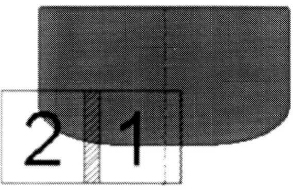
Fig. 15.2 Location of the flow field sections (1 and 2) with respect to the hull transverse section

Figures 15.3 and 15.4 present the details of the PIV set-up. The set-up was situated aside the towing tank. Figure 15.3 presents the model ‘A’ attached to the towing carriage as it passes the PIV set-up. A view of the PIV set-up, just before the model enters it, is presented in Fig. 15.4. In the bottom part of Fig. 15.4 one can notice a laser sheet illuminating seeding particles dispersed in the tank water. The laser beam optical guiding system as well as the submerged CCD camera is also visible. The tank water in the measuring area is seeded before every single measurement.

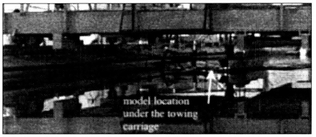
Fig. 15.3 Model ‘A’ under a towing carriage passing the PIV set-up

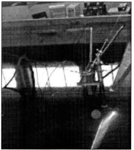
Fig. 15.4 Laser sheet illuminating measurement area with seeding particles dispersed in tank water

15.3 PIV Method

Measurement of flow field with PIV method is based on calculating of displacement of seeding particles between two images, which were captured with camera, in known time interval.

Seeding is brought into the measurement area. Measurement area is lit with ‘laser sheet’. Two images, with seeding particles lit by the laser, are captured. Captured images are divided in to interrogation areas. For every interrogation area, the average particle displacement between two images is calculated with a numerical procedure based on cross-correlation. Velocity is calculated with the following formula:

where:

V – velocity of the fluid in interrogation area;

S – average displacement of particles of the seeding between two images;

t – time interval between capturing two images.

Measurement cycle can be divided into following steps:

• seeding selection;
• illumination of the measurement area;
• image capture;
• analysis of the captured images;
• display of the results.

The following sections contain descriptions of each step.

15.3.1 Seeding selection

To make a PIV measurement, fluid has to contain particles that scatter laser light. These particles, which can be either natural for the flow or injected, are called seeding. Size and material of the seeding depend on specific measurement conditions. Seeding particles should be small enough to follow the flow, but also large enough to effectively scatter laser light. It is very important to get proper seeding density. It is known that seeding density should be about 7–10 particles per the smallest interrogation area used (1, 2). Seeding optimization depends on illumination intensity (scattering ability of particles).

15.3.2 Illumination of the measurement area

In the PIV method the measurement area has to be lit by laser beam shaped in so called ‘laser sheet’. Twin double-frequency Nd:YAG laser is a typical laser used in the PIV method. In the measurements described here, two Nd:YAG lasers were used with pulse energy of 50 mJ each. Beams from the lasers are collimated and transmitted to the measuring area with a special optical system. To obtain ‘laser sheet’ from laser beam the cylindrical telescope was used. The thickness of obtained laser sheet was about of 3–5 mm.

15.3.3 Image capture

Every single PIV measurement consists of two images of light scattered by seeding particles from the volume of ‘laser sheet’ captured with digital CCD camera Kodak ES 1.0. This camera enables measurements at relatively high velocities dependent on size of measurement area. Maximum resolution for this camera is 1008 × 1018 pixels. Dimensions of pixels of the recorded image depend on dimensions of the measurement area.

Proper setting of time between capturing two images is crucial for measurement accuracy. This parameter value should be chosen so that each seeding particle will pass approximately one quarter of the interrogation area. Proper setting of time between two images often proves difficult for flow fields with large velocity gradients. Minimum time between capturing two images for Kodak ES 1.0 camera is 2 μs.

The example of a pattern of seeded particles in the flow around screw propeller model illuminated with laser sheet and recorded by digital camera is presented in Fig. 15.5.

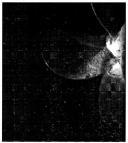
Fig. 15.5 Example of seeded particles image recorded by digital camera in the flow around screw propeller model

15.3.4 Analysis of the captured images

After capturing two images the numerical methods (correlation analysis) have to be applied to get velocity field. The purpose of the correlation analysis is to derive mean displacement of seeding particles between area from first image and area from second image corresponding to area from first image. First the captured images are divided into rectangular interrogation areas dimensions, which are from 8 up to 128 pixels. This rectangular fragment of image is represented with image brightness function, f(m,n) for area from first image and g(m,n) for area from second captured image corresponding to area from first image. Discrete cross-correlation function is described with formula:

Co-ordinates of correlation function represent displacement between image brightness function of first and second image. If seeding particles displacement will be close to each other for particles in one interrogation area then correlation function has high values for these displacements. Correlation not corresponding to particle displacements becomes measurement noise. Noise is increasing with the increase of particles, which have been only on one image (they go in to or go out from interrogation area in time between capturing two images). With high signal to noise ratio one can take the co-ordinates of the correlation function maximum as the mean seeding particle displacement in this interrogation area.

To speed up calculations it is convenient to use one of the properties of Fourier transform (FFT):

Where S(u,v), F(u,v), G(u,v) are Fourier transforms of functions s(m,n), f(m,n), g(m,n). With the FFT algorithm it is possible to transform the image brightness functions f(m,n) and g(m,n). Next one can calculate transform correlation function S(u,v) with the formula mentioned above. Finally with the inverse Fourier transform one can get correlation function s(m,n).

15.3.5 Display of the results

As a results of analysis of images flow velocity fields and seeding density distribution in measurement area are obtained. Additionally, it is also possible to calculate from obtained results vorticity fields, streamlines pattern, and for statistical calculations standard derivation distribution. Results prepared in this way describe the investigated flow very well.

15.4 Discussion of the results

As it has been stated above the most meaningful aim of the experimental research carried out within the frame of the project was to provide the information concerning velocity field in the flow around the ship hull model towed in the tank. Among others the PIV method has been used for this purpose. As the research project was focused on the investigation of the mechanisms of vortex generation in the flow around the ship hull, thus it was necessary to measure transverse components (with respect to the hull symmetry plane – see Figs 15.1 and 15.2) of the velocity field. Therefore, the application of PIV method, which by principle serves as the source of two-dimensional data concerning the velocity field in a flow, seemed to be perfectly suited to this task. Moreover, it is advantageous to use the PIV technique when both velocity components are of the same order of magnitude. In the case of flow around the ship hull model, the longitudinal velocity component is dominating and additionally both of the transverse components are of the same order.

The application of the PIV technique in such a large liquid volume as the towing tank brought numerous difficulties and required solving different practical problems. In order to carry out the experiments it was necessary to:

• paint the ship model side with black dull paint;
• introduce carefully the seeding particles into the water before each model run;
• reduce the ambient light intensity;
• wait until the tank water became calm between two successive model runs.

According to the aim of the experiments, explained in the previous section, the results can be divided into three groups:

• investigation of the influence of the ship hull geometry on the transverse velocity field maps – three different types of the ship hulls were examined;
• investigation of the so called ‘scale effect’ on the way of examination of the velocity field in the flow around two differently scaled models of the same hull;
• examination of the influence of the screw propeller as well as bilge keels and turbulence stimulators on the flow around the ship hull model.

The following sections contain the description of the results referring to the above classification.

15.4.1 Three different hull models – investigation of the velocity field

Three selected types of the hulls, i.e.: A – LNG ship, B – tanker, and C – container differ from each other significantly. Therefore, it has been expected that the images of the velocity field sections will follow those differences. The results of measurements are gathered in Table 15.2. The letter and the number denote the images displayed in the Table. The letter refers to the model type and the number corresponds with the location of the section with respect to the hull (see Fig. 15.1). Each column of the table refers to the same model, and each row to the same flow field section. The table contains the results referring to the section denoted by ‘1’ in Fig. 15.2. The various lengths of the models and the distance between the successive sections are the same, therefore, the total number of sections is different for each model.

The images displayed in Table 15.2 present streamline patterns. The differences can be easily recognized in each row of the Table. As the container ship hull is the most slender one the velocity field seems to be the smoothest. The differences between the flow cases can be also recognized within the wake region.

Table 15.2 Comparison of streamline patterns for three different types of hulls

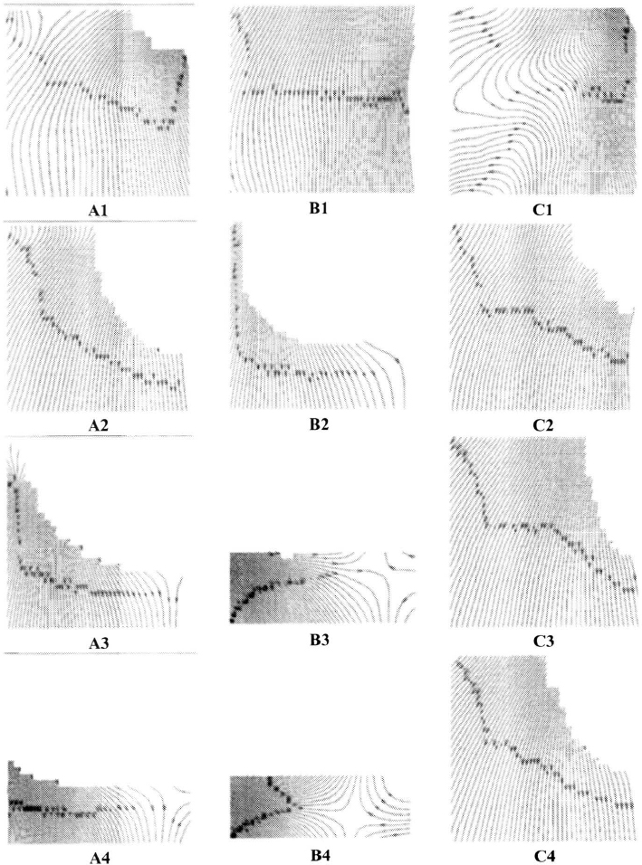
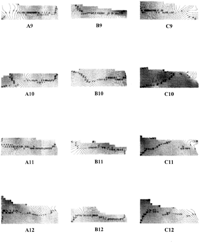
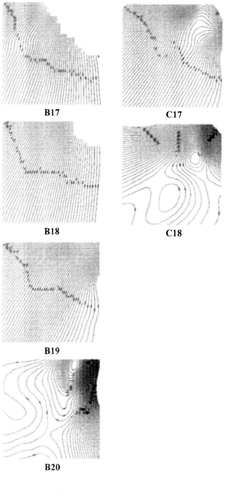
The traces of vortices forming below the bottom of the ship hull can be found in the diagrams B3 and A5. In all of three examined flow cases vortices can also be easily found in the wake field. Nevertheless the hull outline is not marked in the pictures; it can be concluded that the use of the PIV method in the closest vicinity of the hull surface is limited. The density of seeding particles within the boundary layer region of the flow was insufficient to record the reliable scattered signal.

15.4.2 Two different model scales

The LNG ship hull model was selected for testing in two different scales, i.e.: 1:32.8 and 1:16.4. The hull model manufactured at the 1:16.4 scale is denoted by A′. The model A′ was towed with the constant velocity 2.1 m/s. The comparison of the velocity field obtained for both scales is presented in Table 15.3. The left column of the table refers to the model A and the right one to the model A′. Each row of the table contains the results of measurement corresponding to the section located identically with respect to the hull in both cases. The notation used in Table 15.3 is similar to the one used in Table 15.2. The diagrams in Table 15.3 present the two-dimensional velocity vector maps.

Table 15.3 Comparison of the velocity fields measured in the flow around the LNG ship model tested in two different scales

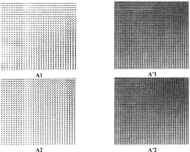
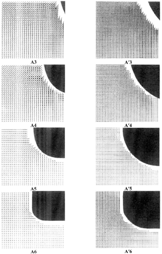
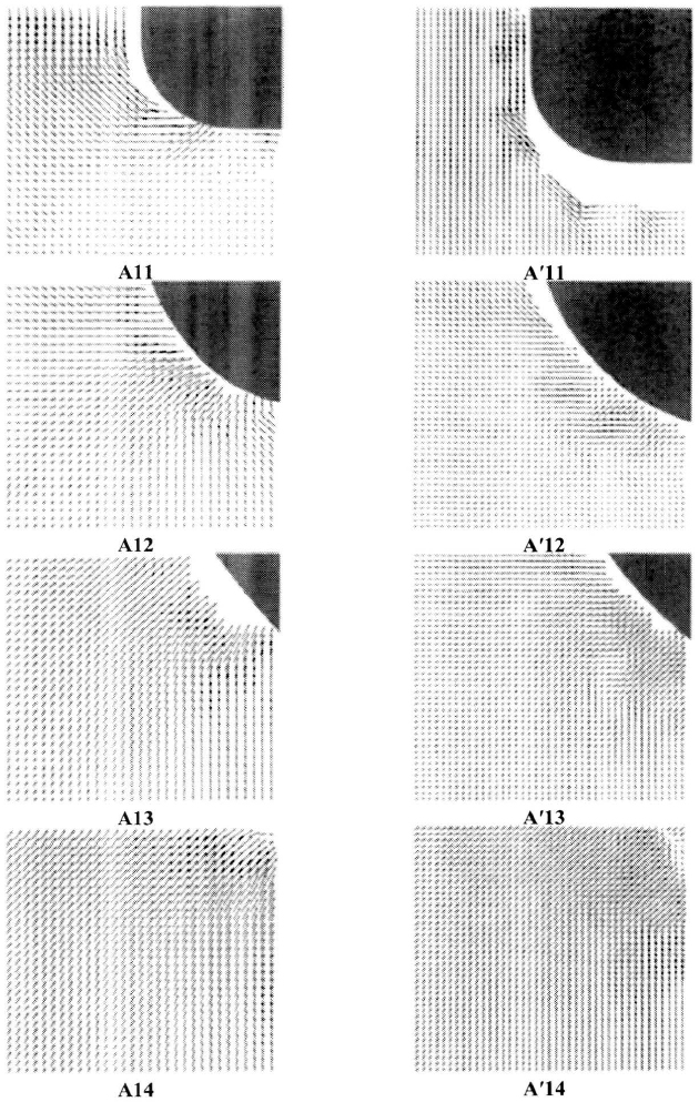
The influence of the model size on the character of the flow can be noticed starting from diagram A9. The Froude number in both flow cases was the same and was equal to Fn = 0.28 therefore, the wave pattern generated by both hulls was similar. Consequently the flow around the bow part of the hull is almost identical (see Table 15.3 diagrams A1–A8 and A′1–A′8) The identity of the Froude number does not coincide with the identity of Reynolds number. Thus the differences between velocity fields can be noticed in the midship region, where the boundary layer is already developed and the influence of the waves generated by the moving hull is not so significant. Some differences between velocity fields referring to both scales can be also noticed in the stern part of the flow region where the viscous effects are dominating.

15.4.3 Screw propeller, turbulence stimulators, bilge keels

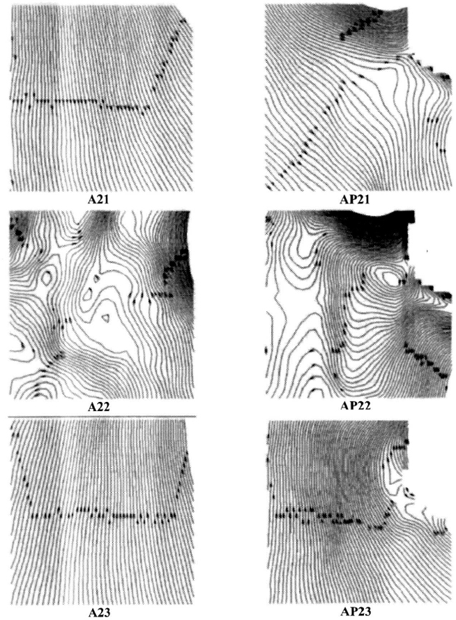
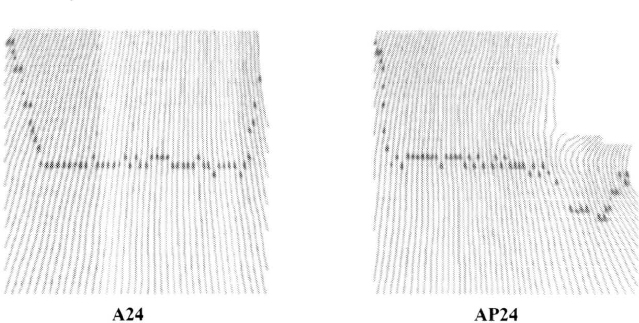
The hull model A was also tested equipped with the screw propeller. The propeller was the four bladed B-Wageningen series model with diameter equal to 120 mm. Its number of revolutions was equal to 500 r/min. The measurements of the velocity field in the operating propeller vicinity were carried out in order to examine the capabilities of the PIV system.

The examples of the streamline maps are presented in Table 15.4. The notation used in the table is the same as in previous tables. The left column (diagrams denoted by the letter A) refers to the ‘bare’ hull and the right one (diagrams denoted by letters AP) refers to the hull equipped with the propeller. The numbers of diagrams correspond to the numbers of successive sections of the flow domain.

The difference between the velocity field is distinct. The influence of the screw propeller on the velocity field within the wake can be easily recognized.

Table 15.4 Comparison of streamlines behind the ‘bare’ hull (left column) and hull with operating propeller (right column)

In order to assess the sensitivity of the PIV method to the hull modifications were introduced and the additional measurements were carried out. The model B was equipped with the turbulence stimulator located behind the bow and the model C was equipped with a pair of bilge keels. The modifications of the hulls are presented in Figs 15.6 and 15.7.

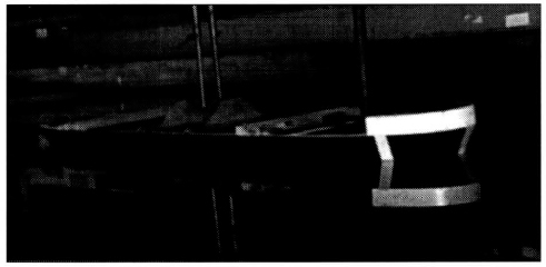
Fig. 15.6 Model B on the water with the sand-strip turbulence stimulator behind the bow

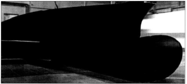
Fig. 15.7 Bilge keels assembled on the side of the hull model C

The influence of turbulence stimulator on the velocity field is presented in Table 15.5. The left column presents the results of the velocity measurements obtained for the hull without the turbulence stimulator (diagrams denoted by letter B) and the right column contain the results for the hull with the stimulator assembled (diagrams denoted by letters BTS). The numbers of frames refer to the successive sections of the flow domain.

Table 15.5 The influence of turbulence stimulator on the character of the flow around the ship hull model

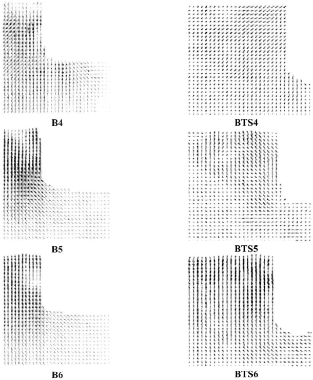
The sand strip turbulence stimulator was located on the hull surface just behind the section No. 4. Nevertheless it is impossible to determine the velocity field in the closest vicinity of the hull surface the modification of the flow due to the turbulence stimulator can be deduced from the comparison of the frames B5 and BTS5.

The last cluster of the PIV measurement results is presented in Table 15.6. In this case the side of the hull model C was equipped with the pair of bilge keels (see Fig. 15.7). The purpose of placing bilge keels on the hull model surface was only to examine the sensitivity of the PIV method. In practice the bilge keels are assembled in different locations. The analysis of the results leads to the conclusion that the PIV technique enables recognition of the influence of ship hull appendages on the velocity field. Two cases are compared: the bare hull model (the left column – the diagrams denoted by the letter C) and the bilge keels equipped model (the right column – the diagrams denoted by the letters CBK). The numbers correspond with the successive sections of the flow domain.

Table 15.6 The influence of bilge keels on the flow around the ship hull model

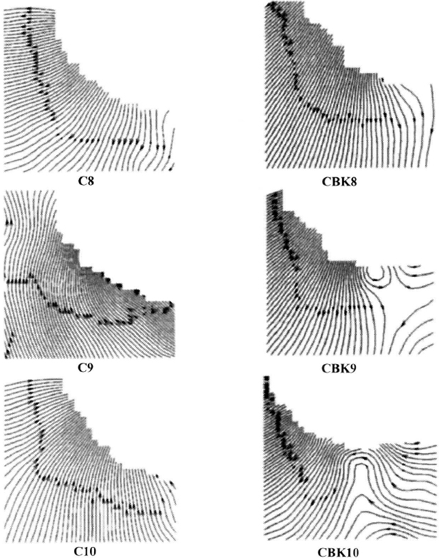
The influence of the bilge keels on the streamline patterns is recognizable starting from the frame No. 9. Thus the PIV measurement technique proves its suitability for the precise measurements of the velocity field in the flow around the ship hull model in the towing tank. The bottom bilge keel reverses locally the flow and generates vortices (see frames CBK9 and CBK11).

15.5 Conclusions

PIV measurements of the velocity field in the flow around the ship hull model in the towing tank were far more difficult then PIV measurements in cavitation or wind tunnel. The most difficult problem was selection and proper distribution of the seeding in measurement area because of the large size of the towing tank. It was impossible to inject seeding properly in the whole tank. Also large quantities of seeding had dissipated laser light scattered on seeding particles in the measurement area before they reached the camera. Only proper quantity of seeding in selected volume gives reliable results.

PIV measurement technique provides two-dimensional information concerning velocity field in the flow. The PIV method enables precise recognition of the velocity field especially when both velocity components are of the similar order of magnitude. Therefore the application of PIV technique for determination of the transverse velocity field in the flow around ship hull model towed in the tank seems to be very promising. Basing on the results of PIV measurements in the towing tank it can be concluded that:

• PIV technique provided reasonable and repeatable data concerning velocity field;
• the sensitivity of the PIV method meets the requirements of ship model testing practice;
• PIV method was successfully applied for measurements of velocity field in the flow around operating screw propeller model;
• the form of the PIV results enables easy comparison with the numerical calculations.

References

(1) Tukker, J. et al. Wake flow measurements in towing tanks with PIV, 9th International Symposium on Flow Visualisation, Glasgow 2000.

(2) Westerweel, J. What is PIV?, Delft University of Technology 1998.

J Dekowski, M Kocik, J Podliński, J Wasilewski, and J Mizeraczyk

Centre of Plasma and Laser Engineering, Institute of Fluid Flow Machinery, Polish Academy of Sciences, Gdańsk, Poland

L Wilczyński and J Kanar

Ship Design and Research Centre, CTO, Gdańsk, Poland

J Stąsiek

Faculty of Mechanical Engineering, Technical University of Gdańsk, Poland