CHAPTER

3

Moving/Using Data

In Chapter 2, you learned about many of the ways to move data within one Oracle database environment. We will now delve into the ways to move and query data from one Oracle database to a completely new Oracle database environment. We will also discuss some of the ways in which to move data from an Oracle database to a non-Oracle database, or even from a non-Oracle database environment to an Oracle database.

You can imagine the many different business cases with the need to get some data residing in one database and combine that with data residing in another. A variety of methods can be used to move that data. We will start off with simple database links when talking about Oracle databases and then move on to Oracle gateways when talking about non-Oracle databases. We will finish up the queries with a short look into materialized views.

In some instances you don’t just want to query data from one database to another but you actually want to move the data from one database to another. A variety of different tools can be used to do this. The tried-and-true export utility can be used to move data from one Oracle database to another Oracle database. Although the export tool is simple and easy to use, there are some drawbacks to it. Oracle Data Pump is a newer tool meant as a replacement for the export utility along with new enhancements. The transportable tablespaces feature was developed to allow whole tablespaces to be moved at one time. This method has a few restrictions, but it allows bulk data to be moved quickly and efficiently. Oracle 12c offers a new method of moving whole databases called pluggable databases. This new feature builds on transportable tablespaces, allowing whole databases to be migrated. We also will look at some of the real-time replication tools. These tools can be used for replicating data from one Oracle database to another Oracle database, or in some cases from Oracle to non-Oracle databases. These tools—Advanced Replication, Streams, Oracle GoldenGate, and the XStream API—all have their pluses and minuses, depending on what your needs are. Some of these tools are historical and have been deprecated, and some are the future direction of Oracle technology.

Database Links

Database links provide a great way to allow users to query other databases from within their own database. For the purposes of this chapter, we will call the other database the remote database. Most organizations these days have a variety of specific built Oracle databases. One database might support a certain finance application, one for a web application, and another for a human resource application. There are times when a report may need to be run that requires information from each of these databases. This is exactly where database links come in. Users can even query the remote database without having a user on that database. This method can be extremely useful if there are a few tables on the remote database that you want users on the local database to access but don’t want to give those users full access to the remote database.

When creating a database link, you have two options: you can have a private link, which is only available to the user who created that particular link, or you can have a public link so that all database users will have access to that link.

Further, there are three different methods of creating the link. A user can connect as a connected user, which means they would need an account on the remote database and would connect with their own username and password. A user can also connect via what is known as a fixed user link. With this method, any user using this link will connect to the remote database as the user specified in the link. All rights and privileges would be associated with the named user in the aforementioned link, and not from the user in the source database. Database links are not typically created by users; in fact, rare is the occasion that users would have a need to create them. They would normally be created and maintained by DBAs to be used by users and applications.

The following will create a database object named REMOTE_DB in the user’s schema. (You can give it any name you want, but having one that makes sense is always helpful.)

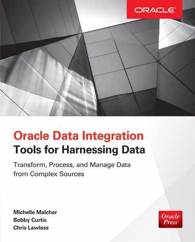
Here, REMOTE_DATABASE_TNS refers to the TNS service name that must be set up in your TNSNAMES.ora file, which is a file that allows users to connect to databases.

NOTE

TNSNAMES.ora is a file that normally lives in the $ORACLE_HOME/NETWORK/ADMIN directory. The file contains information that allows connections to databases. The official name is “net service name,” often shortened to service name or in some cases tnsname. A sample name might look like this:

The following link is very similar to the previous one; however, when a user connects to this database link, it will connect as the user hr:

In the previous example, the user that connected would need to have a user account on the remote database. This example would be as if you were logging on as the user hr in that database. This means that you would not need to set up a personal user account on that remote database. This example would make it extremely useful to have multiple people connect as hr on the remote database.

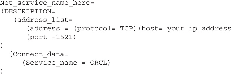
Let’s look at how a user would use a database link. If you wanted to get all the data from a table in the local database, you would type the following:

If you wanted to use the database link, you would use this:

As shown in Figure 3-1, this query will see the @ character and the database link and use that database link to connect to the employees table in the remote database (versus a table in the local database).

FIGURE 3-1. The query being sent to a remote database

You can also take a further step and hide the very existence of a remote database from the user. If you create a synonym for the remote table, the user may never know that the table is actually stored on a different database. Here’s an example:

Database links can be very useful when you have tables in remote databases. Note that queries to database links can be slower than queries to the local database. Not only do you have to consider database time, but now you will have to consider network traffic as well. Therefore, it is important to determine how many times this table will be queried and for what purposes this table and data will be used. It may be better to have a copy of this table in the local database. Having a local copy not only might perform faster, but can help with debugging issues if there are problems with performance. You will have to determine if replicating the table from the remote database to the local database will be worthwhile. We will discuss some of those replication methods a bit later in this chapter.

Database links are also used in other tools and methods regarding data integration. They are often considered a building block upon which many tools rely. Gateways, materialized views, Data Pump, and other tools all can make use of database links. Each of these tools is discussed in this chapter.

Gateways

Gateways are similar to database links in that they allow users to query data from other databases. The big difference is that whereas database links connect to Oracle databases, the gateways allow you to connect to databases from other vendors. The best part about gateways is that they allow users of the Oracle database access to data that they might normally not have access to, including types that are not typically queried through SQL, such as VSAM, Adabas, and IMS. Other SQL-based targets such as Teradata, Microsoft SQL Server, and a generic ODBC gateway are also available.

There are two main parts to gateways. The first is called Heterogeneous Services, which is used by all the different gateways services. The second piece is called the agent, and is different for each of the different target databases. The key is that users do not have to have any knowledge of the different non-Oracle targets—indeed, they may not even know that they are querying a different system. Syntax, location, data types, and so on are all handled by Oracle so that the user can focus on selecting the data they need. This part is very important because SQL syntax can vary from one database vendor to another. Also, data dictionaries can be quite different. Users don’t have to learn other database systems, and application developers don’t need to learn how to modify their application to account for disparate systems. Also, the very fact that it is a different database vendor can be hidden by the use of synonyms.

NOTE

Besides the specific gateways is a generic gateway available for ODBC drivers. Although it does have some limitations, it is available for free and can handle just about any target that accepts an ODBC connection.

To connect to a non-Oracle database from the Oracle database, you use a database link that sets up an authenticated session in the background. When you start making queries, you will be using what is known as SQLService. As part of the Heterogeneous Service, SQLService does much of the heavy lifting for the users. As everyone knows, SQL is the ANSI (American National Standard Institute) standard to which most major database vendors adhere. However, each vendor complies at different levels, and there may be many slight nuances from vendor to vendor. And indeed, some of the gateways will also allow you to connect to non-SQL databases. That is where SQLService comes into play. SQLService will translate from Oracle SQL to the version of SQL on the non-Oracle database. This service will also convert non-Oracle data types to Oracle data types, and vice versa. Keep in mind that some functionality might not be supported, and workaround queries must be performed so that they work on the non-Oracle systems. Lastly, the service will “translate” calls that make notice of the Oracle data dictionary and parse them into the correct system calls on the non-Oracle database target’s data dictionary. Suppose you are remotely connecting to a Microsoft SQL Server database and you make the following query:

This query would retrieve information about the tables residing on the Oracle database. If you ran the same query in a Microsoft SQL Server database, you would receive an error. By going through the Oracle gateway, the query would be translated to a query that Microsoft SQL Server would understand. The data set result would then be given back to the Oracle user in a format that they are likely to recognize.

The mapping of these SQL calls is all done transparently. PL/SQL calls are mapped as well. If the SQL functionality does not exist on the target system, then appropriate SQL statements are made to obtain the same results.

Some commands cannot be translated, and of course some commands you’ll want to run natively on the non-Oracle target. For these occasions, Oracle has developed a special PL/SQL package to do just that. It is called, appropriately enough, DBMS_HS_PASSTHROUGH. Here’s an example:

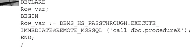
The resulting command will be passed through Oracle, and the procedure (dbo.procedureX) will be executed directly on the target machine.

NOTE

The DBMS_HS_PASSTHROUGH package is really neat. It is very useful when you are making those calls to the target database and need to have that code execute natively on the non-Oracle system. It is probable that you’ll want to search for this package on your Oracle system to learn more about it.

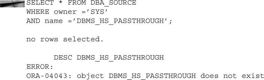
The DBMS_HS_PASSTHROUGH package technically doesn’t exist. It is part of Heterogeneous Services to pass along code through the gateway, but it is not a traditional DBMS package that we are used to dealing with.

To ensure faster service for the non-Oracle target database, much of the non-Oracle database information is stored inside of Oracle. Oracle does this at the time that the gateway is registered with the Oracle database. This prevents Oracle from sending unnecessary commands and queries to the non-Oracle database. The SQL Parser in Oracle will also only parse the SQL statements one time and save the results.

As with database links, the very existence of gateways can be hidden from end users. By using a synonym, you can cause the target table to appear to be just another local table on the Oracle database.

Using gateways is a fantastic way to have legacy information stored on various types of non-Oracle database and make their data available to Oracle. In this way, tables from those other systems can be joined with Oracle tables to give users useful information.

Materialized Views

Introduced in Oracle 7.3, materialized views have been enhanced several times in later releases. Prior to version 8i, materialized views were called snapshots. Before we delve into how materialized views work in the data integration space, we will go over some of the basics. A view is a database object that is a query stored in the database. When you run a query against the view, the underlying query is run. A materialized view, on the other hand, is an object in the database that contains the actual result of a query. In other words, the materialized view takes up physical space in the database, whereas a “regular” view does not. Typically, materialized views were created to help with query rewrites in data warehouses. However, clever DBAs have discovered that materialized views can also be useful in regard to data integration.

Let’s look at creating a simple materialized view. Consider the following example:

Of course, there are many options we have not covered, and typically, materialized views do not simply select all the rows from one table. A typical materialized view may contain joins of multiple tables or have aggregate functions involved. The point here is to show that a materialized view is created much like a regular view.

So knowing that a materialized view takes up space much like a physical table, the next logical question would be, why not just create a table instead? This is where the “specialness” of materialized views comes into play. Once a table has been copied, at that point in time the two tables are 100 percent the same. However, if someone were to insert a row into the original table, it would have one more row than the copied table. From there on, the tables would start to diverge. With a materialized view, different methods are available for keeping the view updated using any DML changes made to the base table(s). This is done through the REFRESH parameter options. There are two basic methods of refreshing your materialized view: incremental refresh and complete refresh.

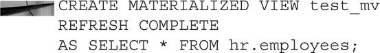
A complete refresh sounds like exactly what it is—a rerun of the SQL used to create the original materialized view. The SQL statement that the view is comprised of will be executed and the materialized view will be populated again. If it has complicated SQL joins or a massive amount of data, a complete refresh can take quite some time. Complete refreshes can be called at any time, or you can have them occur automatically. Here is an example:

As before, our materialized view is a full copy of the hr.employees table. This time we have added a few parameters. The materialized view will be populated right away because of the BUILD IMMEDIATE clause. The part of the SQL referencing REFRESH COMPLETE will be like the preceding statement that the complete view will be a refresh versus a partial refresh. The refresh will only occur when a user requests the refresh, hence the ON_DEMAND statement.

The following materialized view would only be initially populated on the first request for a refresh; otherwise, it would be empty:

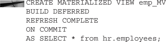
Note that we have left the REFRESH COMPLETE the same. Also, ON COMMIT means that every time there is a committed change on the base table, the materialized view is completely refreshed.

So let’s compare these options. We can do the initial build right away, or we can wait for the very first time a refresh is requested. This is controlled by the BUILD IMMEDIATE or BUILD DEFERRED option. The other option is ON DEMAND or ON COMMIT. Building the materialized view “on demand” is just that—as a user calls for the materialized view to be rebuilt. The other option, ON COMMIT, means that every time a change is made to the base tables a committed refresh is done. Imagine having very large base tables and asking for a complete rebuild every time a commit is done. This is where we get into the next options on how the refresh is done.

In the earlier examples, we had the option REFRESH COMPLETE. We also have the choice of REFRESH FAST. This means that rather than getting all of the data, it will only get the data that has changed. This is extremely useful for tables that are very large. There are a few restrictions with REFRESH FAST, however. The major one is that you will have to create a materialized view log. When a DML change is made to the base table, a row will be stored in the materialized view log. The materialized view log would then be made to refresh the materialized view. The log is stored in the same schema as the view.

Now that you have seen how the basics of materialized view work, let’s dig into how they can be useful in different ways when used with data integration. Let’s suppose that you had a local database and one table on a remote database that you wanted to bring over locally. Earlier we looked at how to use a database link to make a query on a table in a remote database. Now we’ll look at a method to bring that copy of the table to the local database using a materialized view:

This example creates a materialized view in the local database that’s based on a table from the remote database. Notice the use of a database link. The initial loading of the table will occur at creation, and this would be a partial refresh of the changes only upon every commit on the remote side. Care should be taken to see if querying the remote database would be faster than using the materialized view. Also, other replications offerings may be better suited to the task. It will depend on your needs. Some DBAs have used materialized views to migrate tables from a remote database to a local one without a large amount of downtime. As shown in Figure 3-2, copies of the table are sent over the network using a database link and created on the target database. Using a materialized view may not be the best method to perform a low-downtime migration because of the availability of other Oracle tools, such as Streams and Oracle GoldenGate. However, a materialized view can provide this functionality if needed. Check to see the performance impact of the source database and the network impact before proceeding.

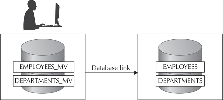
FIGURE 3-2. An example of how to migrate to another database with a materialized view

Materialized views provide a great way to move data and also to pre-position the data in data warehouses. It is also a great method for joining multiple tables together in one physical location, especially if you have a need to aggregate this data. And as you have seen, materialized views can also provide a way to transfer data from one database to another, including data migrations.

Export/Import

The simplest way to get data out of an Oracle database is to use the DBA’s tried and trusted friend, the export utility. This utility has been around since at least Oracle 5. It is a very simple tool to use and extremely effective. Most DBAs have this tool in their toolbox and use it. There have been many enhancements over the years, and we will discuss some of the newer ones. Technically, the export utility has gone by the wayside and is a legacy tool now that Data Pump is here, but many people still use export because they have used it for such a long time and are familiar with it. The export functionality has been incorporated into Oracle Data Pump, and export is technically deprecated and will not work with certain newer data types.

Export provides a good way to move data from one Oracle database to another Oracle database. One great feature is that the Oracle databases can be different versions (with some caveats) and on different platforms. For example, you can export the data from an Oracle 10.2 database on Windows and import that data to an Oracle 11.2 database on Linux. The cross-platform nature of export makes it extremely flexible and usable. Exports are very useful for taking “snapshots” of certain tables and/or schemas. Often these export files cans be used as backups in case the objects are accidently dropped. An export should not be considered a complete backup, and other precautions should be taken; however, it can be a useful method as part of an overall backup strategy.

Export files are binary files that reside on the operating system of the disk. These binary files can only be read by the Oracle import utility. There are three different methods for interacting with the export utility. Figure 3-3 shows an example of the export dump file being created on the operating system. You can invoke export from the command line, interactively from the command line, and via parameter files. The task at hand will determine which method is chosen. Typically, the parameter file option will be used by most DBAs in an operation mode.

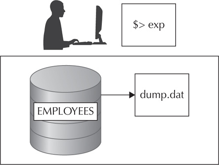
FIGURE 3-3. Exporting a file from the database

Invoking Export from the Command Line

You can specify all the parameters for the export command on one line:

This will produce a file called sample.dmp. That binary file contains the data for the database table departments from the hr schema. You could then take that .dmp (dump) file and ftp it or somehow move it to the intended target machine and then import it into the database, like so:

To get a list of the many options available for export and import, you can run the utility with the help flag set to get all available options:

Invoking Export Interactively from the Command Line

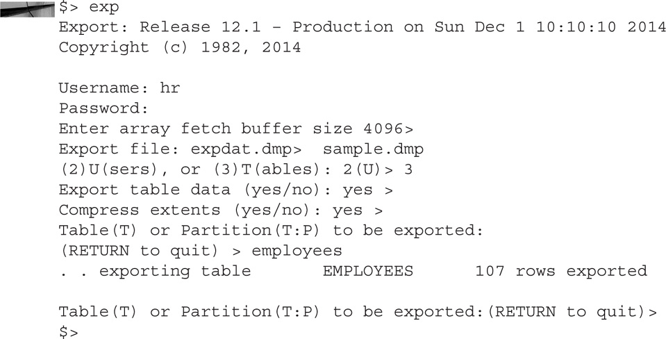
Although it’s not a very common method, you can also invoke the export utility in interactive mode. Rather than feeding all the required information to the utility up front, you are prompted for all the required information needed to complete the export. You will be given default options, and you can press ENTER (RETURN) to accept the defaults or type in your own answers. Here’s an example:

You will see that you now have a file on the operating system called sample.dmp. This file can also be imported interactively, like so:

Interactive mode is very easy to use and is nice for simple exports/imports. However, it only asks for some of the basic parameters and does not cover all the parameters available.

Invoking Export via Parameter Files

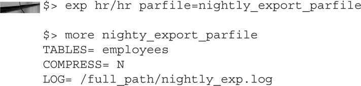
The most common way that people deal with the export/import utility is via parameter files. By placing all your parameters that you would normally use inside a file, you can call the export utility as needed. You would start the utility and use the parameter file to call all the parameters contained therein. For example, suppose you like to export a certain schema every night at 1:00 A.M. You could use a cronjob to call the parameter file at 1:00 A.M. every night, like so:

The file could then be imported the same way:

Export files, as mentioned earlier, are “snapshots” in the time of when the export was taken. But what if the table has data “in flight”? Some exports can take quite a bit of time to perform depending on the volume of data. What if rows have been added or removed, or values have changed in the table you are exporting? This can result in exports that are not consistent. For this reason, Oracle developed a parameter called consistent. You would set this parameter so that all the tables listed would be from the same point in time. You also need to ensure that you have enough UNDO tablespace and that the retention period is long enough to support the volume of data. Consider the following example:

This ensures that the tables are from the same point in time. This is especially important if you are exporting tables with foreign key/primary key relationships.

In earlier examples we were exporting just one table. Exports are not limited to one table. You can export multiple tables:

You can export whole schemas:

You can export whole schemas minus certain tables:

You can also export the metadata without the actual data itself:

The whole database itself can be exported:

NOTE

The full database export is a very powerful feature that has been used for a long time. Now that the transportable tablespace and pluggable databases features are here, these options may be better suited to moving whole databases. These two features are discussed later in this chapter.

To import these files, you use the same method as before. Figure 3-4 shows the binary dump files being sent from the operating system into the database. Two parameters we want to make a special note of are the FROMUSER and TOUSER parameters. These parameters are often misunderstood. When you are logging on to do an export, you are logging on as a user. That may or may not be the same schema you are exporting. The same holds true regarding importing. The user doing the import may or may not be the schema you are importing tables into. For this reason, the two parameters are used. If you are moving the data from schema User1 and want to put that data into User2, you would make use of the FROMUSER and TOUSER parameters. Here’s an example.

FIGURE 3-4. Importing a data file into a database

When you export whole schemas, you will get all the objects inside those schemas. You can choose whether to export/import statistics, indexes, grants, constraints, and other options. Consider each of these carefully. Each will depend on exactly what you are trying to achieve.

We have one last command to discuss. The SHOW parameter for import is a useful feature for checking on things before performing the actual import. Here’s an example:

Note that the import will not perform but rather will show the contents of the export file to the display screen. The SQL operations are displayed in the order they would be used. This may be useful as a check before you perform the actual import.

As you can see, the export utility provides a great way to move data into and out of Oracle databases. There are some limitations, of course. Oracle addressed many of these limitations when it came out with the Data Pump utility, which grew out of the export utility. Data Pump is Oracle’s way forward, and export/import are considered legacy products. We will explore the Data Pump tool next.

Data Pump

The Data Pump utility was introduced in version 10g of Oracle as the future direction for the export and import utilities. Lots of great features were introduced, and of course Oracle keeps coming out with useful new features with each subsequent release. Think of it as doing everything that export/import can do, but more. It’s the export utility on steroids. One of the really great features is that when Data Pump runs into an error, the job will be paused; you can fix the error and then resume the Data Pump job. This is a huge advantage over export/import, where if the job fails, you have to clean up and then start over. There are some setup and privileges that need to be granted to users before they can use Data Pump. Data Pump also makes use of two PL/SQL packages in addition to the command-line utilities. These packages are DBMS_DATAPUMP and DBMS_METADATA.

Data Pump also has a variety of ways to actually move the data. The transport tables feature just moves the metadata for the tables, not the actual data. We cover transport tables in the next section. The next method is Direct Path, which skips the SQL layer of Oracle and has a server process move the data from the dump file to the target. This is the fastest method and the default. There are a few data types that Data Pump does not support with the Direct Path method. If Direct Path is not available, the external tables are used. You learned a bit about external tables in Chapter 2. The conventional (or “old”) way of doing things would be used if Direct Path or external tables are not allowed. Lastly, we have the network link, which does not create a dump file but instead streams the data over the network. We cover it in a bit more detail later in this chapter.

The first point we need to discuss is the fact that Data Pump needs to have a default location to place the files, logs, and SQL files. This is done via a directory object. This object specifies the location of the directory path, like so:

You will also want to make sure you have given the two roles of DATAPUMP_FULL_DATABASE and DATAPUMP_IMP_FULL_DATABASE to users who plan on using the Data Pump utility. Like the export utility, Data Pump has a variety of parameters to help you control certain aspects of how it works:

Notice that the command is now expdp versus exp. Similarly, the command is impdp versus imp. You can now ftp the file over to the target, just like you did earlier. Like export, the Data Pump utility has three operating options: command line, interactive mode, and parameter file.

One of the frustrating things about the export utility is that if you have five tables in a .dmp file and you run into a problem on the fourth table during the import, you have to start all over again from the beginning. Data Pump rectifies that situation and has a start/stop function that allows you to resume where you left off. Thus, if an error occurs, you can pick up from where you left off.

One of the great advantages of Data Pump over export/import is the networking feature. This allows you to set things up so that rather than having Data Pump land a file on the source operating system and your having to ftp that file over to the target, Data Pump will stream that file over to the target itself. Let’s look at an example. The following import command would be run from the source side:

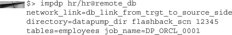
It makes a call to the target instance using a TNSNAMES service name of remote_db. The network link is a database link on the remote database that points back to the source database. When the import is run, it connects to the source database (via the database link) and imports the data for the employee table from the Oracle SCN 12345.

A few powerful things are going on here. First, there is no export command. All of this is being done from the source side. This makes setting up Data Pump scripts very easy, with just a little bit of setup with database links. Conversely, we could run a similar command only on the target side and have it reach back over to the source side with only a reference to the database link.

Also note that the import has a name—in this case, DP_ORCL_0001. The Data Pump utility will automatically give a name to a job. Alternatively, you can use the parameter JOB_NAME to give it one yourself.

NOTE

If you don’t know the name of a job you can look it up here:

While a Data Pump is running, you can stop it in the middle. Press CTRL-C, and you should get an export prompt. Make sure you get past the Oracle banner before pressing CTRL-C. When you see the export prompt, you can work interactively with Data Pump. From another terminal session, run the following:

Now if you flip back to the terminal session that has the Data Pump job running, you can start, stop, or kill the session. This can be useful when dealing with certain problems. Maybe you learned that a large batch job is going to happen and you don’t want your Data Pump job to interfere, or you learned that there is a temp space issue. In this way, you can pause, resume, or even kill the session as warranted.

The Data Pump utility is also backward compatible with all the export commands. If you type in older parameters such as OWNER, Data Pump will correct it on the fly and put the new parameter (SCHEMA) in its place. This allows you to keep all your old export scripts without needing to rewrite them.

Data Pump builds upon all the great things that the export utility could do, but adds so much more. The networking features alone are a huge advancement. Data Pump can now use a variety of different methods. The wider parameters allow for customization and speed, and the new features incorporating transportable tablespaces and external tables make Data Pump a very powerful tool in the data integration space.

Transportable Tablespaces

When transportable tablespaces first came out in Oracle 8i, people saw the immediate benefits of being able to move whole databases at a time. Like the other features mentioned, transportable tablespaces is enhanced every version that comes out. Some business benefits of moving these tablespaces together versus just exporting at the schema or table level include moving a tablespace to a data warehouse, performing tablespace point-in-time recovery, performing database migrations and platform migrations, archiving historical data, and keeping a read-only copy on another database.

Starting in Oracle 11g, Data Pump is now the method used to transport tablespaces. The tablespaces that are to be moved must be in read-only mode (there is the exception of moving them from a backup). Also, starting in 11g, you can now do certain cross-platform migrations; this was a huge step forward in the technology because it allowed this great feature to move on to newer and different operating systems. There are certain restrictions when you’re moving tablespaces, but with every release that list grows smaller.

Prior to performing the actual migration, we need to ensure that the tablespace is self-contained. This means that there are no dependencies between the tablespace being transported and those not being transported.

Then we will check to see if there are any items that have dependencies that would not allow us to make the move:

If there are zero rows, that means that the tablespace is self-contained and we are able to proceed.

Let’s walk through the actual movement of a tablespace migration. After making sure that the tablespace is eligible for movement, the next thing we must do is to make the tablespace read-only:

This can be a big drawback to many DBAs who want their data to be accessible 24/7. However, the requirement makes sense because we want a consistent view of the data, and the transportable tablespaces method of moving data is much faster than other methods. If making the tablespace read-only is a problem, you may have to look at other methods. As mentioned, those other methods may be slower. It will be a trade-off between downtime and speed.

Now that we have ensured that no changes will be made to the objects inside the tablespace, we are ready to start the actual migration:

Earlier in our discussion of the export and Data Pump utilities, we talked about the dump files containing actual data inside them. With the method we just used, only the dictionary metadata about the tablespace would be put in the dump file. This means that the performance is vastly superior to exporting the actual data. The dump file will also be relatively small compared to a full data file.

Once the command has completed, we take the emp_data.dmp file and move it to the target system. There are a variety of ways to move these files. We could ftp them or use any other method to move them. For this example, we are assuming that they are not in ASM and are the same endianness. If the source and target are of different endianness, we would need to use the RMAN convert command.

NOTE

If you are moving from a big-endian platform such as AIX to a little-endian platform such as Linux (or vice versa), you will have to perform a conversion before you do the migration. You can use the built-in backup tool RMAN to perform the conversion. You will need to convert the logical tablespaces or the physical data files. You can convert them on the source (tablespaces) or convert them on the target (data files).

We also have to move the physical data file(s) that are on the disk. We need to find out which data files belong to the tablespace emp_data:

We then take that physical data file and move it to the target machine, just as we did with the emp_data_dmp file.

Once the data files files are copied to the appropriate places, we run the import command on the metadata file on the target database:

This command imports all the metadata about the tablespace and the objects inside that tablespace. It correlates all this information with the physical data files we moved. Once this import has finished, we are ready to proceed.

Before we moved the tablespace, we made it read-only. We will now take it out of read-only mode so that users can read and write to this target database (we will also want to make sure we do this on the source database as well):

The transportable tablespaces method of exporting whole tablespaces makes the migration process so much easier than exporting schemas and tables. Transportable tablespaces is great for the one-time movement of data. The only drawback is that the tablespaces are placed in read-only mode for the duration of the export. In Oracle 12c, Oracle took this one step further via pluggable databases.

NOTE

You can also convert files from a regular file system and put them in Oracle Automatic Storage Management (ASM).

Pluggable Databases and Transport Databases

Oracle 12c introduced a new concept into the Oracle database world—the multitenant database, which is often called a multitenant container database (CDB). A CDB would contain one or more pluggable databases (PDBs). Think of a company with hundreds of databases spread across 100 different servers. This can be a nightmare to maintain. As advances in hardware are achieved, a DBA may start to consolidate some of the databases on to fewer servers. This is a good idea; however, it just means that multiple databases now reside on one physical machine. The problem with this method is that the databases that are co-located on the same server do not share anything. With the multitenant architecture, these different databases can be consolidated under one structure to share resources more efficiently. Databases can now be plugged and unplugged from the CDB with relative ease. We will discuss the methods of moving these databases.

To move PDBs, you would use Oracle Data Pump along with the idea of transportable tablespaces. Pluggable databases build on the two features you have just learned about. Oracle continually builds upon its past features. The method for moving the pluggable database is very similar to that of the movement of a tablespace.

A target database should be created with the CREATE PLUGGABLE database command. This is a new feature in 12c. As before, all of the tablespaces should be placed in read-only mode, like so:

The physical data files for the corresponding tablespaces should be moved to the target database operating system. The export command will have two new parameters introduced:

This is followed by the import:

At this point, you would change the target tablespaces to read write, and you are all set.

Logminer

Logminer is not exactly a tool used to move data, but it is a tool to help you learn more about transactions in your database as well as help troubleshoot potential problems with data integration. Therefore, we will look at some information about logminer and an example of how to use it.

Logminer the tool was introduced in Oracle 8 and then greatly enhanced in Oracle 9i. Much of the enhancements in Oracle 9i coincided with the extra information that is now stored in the Oracle redo logs. As you know, Oracle redo logs contain a history of changes in the Oracle database. The primary purpose of those redo logs is for database recovery, hence the name “redo.” When a redo log is filled with data, the log is switched and Oracle starts writing to the next redo log. If archiving is enabled (and in a production database, it should be), the archive process will make a copy of the redo logs called archive logs. The archive logs are a permanent history of changes to the database. In the event of a problem, you can restore all the changes back to the database by reapplying the archive logs on to the most recent backup. However, over the years Oracle has made available more information that can be extracted and queried regarding the redo logs. As Figure 3-5 shows, logminer allows you to peer inside redo logs.

FIGURE 3-5. Logminer used to peer into redo logs

You may want to look into a redo/archive log for many reasons. You may want to undo specific changes made by a specific user. Rather than restore or recover a whole table’s worth of information, you can look in the redo logs and find the specific changes made to perform the reverse DML. You may want to reverse a particular user operation error—for example, a user could have deleted some rows using the wrong WHERE clause by mistake. Some DBAs like to use logminer to help them tune and audit the database in conjunction with other Oracle tools. It gives them more access to the direct data by providing them with another viewpoint into the redo logs versus looking at reports and statistics.

Supplemental logging must be enabled in order to obtain information from logminer. First, we must make sure that supplemental logging is turned on. We can ensure this by checking the v$database view:

If the database is not in supplemental logging mode, we can turn it on:

Now we are ready to start mining the redo logs:

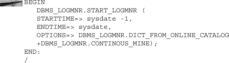
Running this PL/SQL block will allow us to obtain one days’ worth of Oracle redo logs. As with all Oracle DBMS packages, you have many different options to explore. The results from running logminer will be stored in the V$LOGMNR_CONTENTS view. You can query that view to find the information you are looking for:

Be careful: if you don’t specify a WHERE clause, you may end up searching hundreds of redo logs.

NOTE

The contents of V$LOGMNR_CONTENTS are only valid for the user that is running the DBMS_LOGMNR package. Also, the data is only available in that session and will be gone when that session ends. If the data is important, you may wish to copy that data into another table so that it will be available for you to analyze at a future time.

Advanced Replication

When Oracle 7.3 came out, the Internet was young and the future was bright. Advanced Replication was introduced and was an exciting feature. Advanced Replication is available with Oracle Enterprise Edition at no additional charge, and the features are built in and installed on the Oracle server. The odd part was that Oracle kept enhancing Advanced Replication and then introduced Oracle Streams as another replication tool. Like Oracle Streams, Advanced Replication was enhanced as each new version of the database arrived. And like Streams, Advanced Replication is now deprecated in Oracle 12c.

Advanced Replication was older than Oracle Streams, but Oracle Streams had more momentum behind it and seemed to be the favorite among users if they were given the choice. There were two ways to do advanced replication in the past. Snapshots (which were later changed to be called Materialized Views) and Oracle Advanced Replication. Oracle Advanced Replication could be used in two modes. Asynchronous mode takes the DML changes and stores them in a queue held locally until they are forwarded to the targets. This was also referred to as store and forward. Synchronous mode sends you the data on immediately. Due to the fact that it is deprecated and not as popular as Oracle Streams, we will not go into the details on how to set up and configure Advanced Replication. If you have Advanced Replication currently running on your site, you might want to start planning to move to another replication technology.

Oracle Streams

Oracle Streams is a powerful feature that was introduced in Oracle 9i. Each version of Oracle brought on exciting new enhancements. Oracle Streams is provided at no additional charge for Oracle Enterprise Edition customers. However, Oracle announced, when Oracle 12c came out, that Streams is now deprecated. The following is from the Oracle documentation:

“Oracle Streams is deprecated in Oracle Database 12c Release 1 (12.1). Use Oracle GoldenGate to replace all replication features of Oracle Streams.”

Although it is deprecated in 12c, we will have a quick discussion on Streams how it plays into Oracle and non-Oracle environments. Also, because of the large number of customers using Streams, we’ll look at a quick example of how to install a simple Streams setup.

Oracle Streams works on a very simple premise: it captures changes made on tables in the source database and replicates those changes to a target database. Before we delve into some of the details, let’s talk about this replication at a high level. Suppose your source database is an online transaction processing database (OLTP) and you want to have all the changes made to certain tables replicated to a target database. This target database could be a data warehouse, a reporting database, or even a QA or development database that you would like to be in sync with the source database at all times. Every time a DML (or DDL for that matter) is made on the tables on the source database, you would like those DMLs to be replicated to the target. Oracle Streams will be configured to look at the Oracle redo logs in the source database. Any time that there is a change to one of those tables, the Streams capture process will grab that information from the redo logs and put it into something known as a logical change record (LCR). This LCR is then sent over to the target database, where an apply process takes the LCR and applies those changes to the table on the target. You now have real-time replication from the source database to the target database.

Note that some prerequisites need to be set up ahead of time. You will want to create a new user to be the Streams administrator. This user will need certain privileges in order to run Streams. Oracle has a package that grants the privileges needed for Steams, and DBMS_STREAMS_AUTH contains the procedure to do this. We will look at this parameter when we set up Streams in our example.

You will also want to take into consideration some database init.ora parameters. The main parameter, of course, is STREAMS_POOL_SIZE. This will set up a memory area that holds buffered queues as well as the area for internal messages.

First, we will create Streams Admin users on both the source and the target. After this, we will make sure that the user has the proper roles and permissions needed.

After the users have been created on both the source and the target, we configure the actual Streams queue by logging into the source database as the STREAM_USER we created earlier:

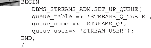
Again, this will be done on the source and then again on the target.

On the source, we make some rules on what information should be captured:

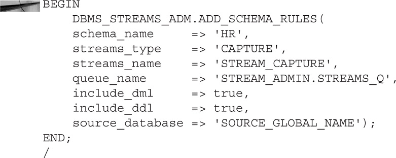
Here we are saying that we want to capture all DML and DDL changes for the HR schema. Those changes will be placed in the Streams Q we created earlier named STREAM_Q. For the source_database parameter, we give the GLOBAL name of the source database.

We now have to create some rules for the target database:

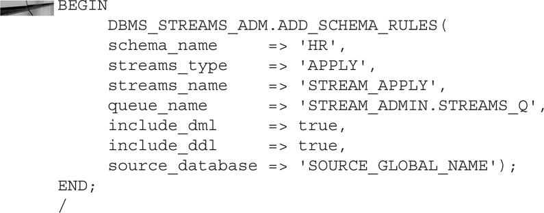
The apply rules are very similar to the capture rules. One difference to note is that the source_database parameter once again refers to the SOURCE database.

Now we just need to make sure to start both processes on the source and target:

This is just a small sample of how to set up Oracle Streams. There are hundreds more parameters and complex rules you can set up. Also, a great feature called downstream capture enables you to have the CAPTURE process sit on a database other than the actual source database. Streams has been well liked because it came with Enterprise Edition of Oracle at no additional charge. However, many DBAs do not like Streams because it has many PL/SQL packages to remember, which sometimes can make administering Streams somewhat difficult.

Oracle GoldenGate

In July of 2009, Oracle announced that it was acquiring GoldenGate. In September of 2009, the acquisition was complete. GoldenGate was born in the Tandem space (now called NonStop and owned by HP) and was simply “the standard” in disaster recovery when it came to Tandem/NonStop computers. For years, customers used GoldenGate for disaster recovery. However, some customers also want to take the data from NonStop databases and share it with other database targets. MySQL, Oracle, Microsoft SQL Server, and Teradata all became targets for GoldenGate. And it wasn’t long after that that customers starting asking for those various databases to also be the sources. GoldenGate grew rapidly once Oracle was a source database, and the rest, as they say, is history.

One of the reasons Oracle GoldenGate has become the number-one real-time data integration tool is because of its flexibility. The fact that the source and target can be different versions of Oracle, different operating systems, and even from different database vendors makes Oracle GoldenGate a great tool. GoldenGate also allows for multiple targets, and having the source and target be completely independent from each other is a huge feature. Because of the importance of Oracle GoldenGate in the data integration space, and because Oracle GoldenGate is the strategic direction of Oracle’s replication projects, a whole chapter is devoted to Oracle GoldenGate: Chapter 5.

XStream API

XStream is a relatively new feature of the Oracle database. It is often confused with Oracle Streams because of the name, and indeed the same XStream API was built on top of the existing Oracle Streams base. An important note: Oracle Streams comes with the Enterprise Edition database at no additional charge, and as previously noted is deprecated in Oracle 12.1. The XStream API was introduced in Oracle 11.2. The use of the XStream API also requires the purchase of an Oracle GoldenGate license. This means that if you plan on developing code that will make use of the XStream API, you will want to determine if using Oracle GoldenGate will solve your replication needs right out of the box rather than developing with a solution with the XStream API.

The XStream API allows for the capturing of changes made to the Oracle database and sending them to non-Oracle databases (or files). It can also do the reverse, taking changes from non-Oracle databases (and files) and inputting them into an Oracle database. The XStream API consists of two aptly named parts: XStream Out and XStream In. In theory, one could use the XStream process to move the data from Oracle to Oracle, although as you have seen there are other methods to do this.

XStream Out

A capture process, much like Oracle Streams, will capture changes made in the Oracle database. These changes are in the same format as Oracle Streams: logical change records (LCRs). XStream Out sends these changes in real time to what is known as an outbound server. An outbound server is an optional Oracle background process. Client applications will connect to that outbound server and receive the information in the form of LCRs, as shown in Figure 3-6. The client application can be configured to receive that data via XStream Java or XStream OCI. The target for the Java or OCI connects may be an Oracle database, a non-Oracle database, or a file system. The client applications will then take the LCRs they have received and deal with them programmatically. The exact method in which they apply or relate with the LCRs will depend on the individual applications.

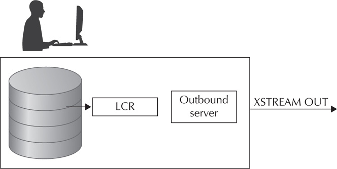
FIGURE 3-6. An example of XStream Out

XStream In

XStream In works in much the same way as XStream Out, but in the opposite manner. A client application will obtain the data from a non-Oracle database, a file system, or some other method, and will forward that data to an inbound server in the format of LCRs. The inbound server will take those changes and apply them to tables within the Oracle database, as shown in Figure 3-7.

FIGURE 3-7. An example of XStream In

As noted, rather than coding the client applications to the various non-Oracle targets, it may be more advantageous for you to see if Oracle GoldenGate supports those different non-Oracle clients to avoid any unnecessary coding.

Summary

As you have seen, a large variety of tools is available to query and move data. Database links, as you have seen, are useful in their own right in helping query tables in remote databases. Notice further that as we looked at gateways, materialized views, Data Pump, transportable tables, and more, many of those features also incorporate database links into their operations. The use of database links is one of the founding principles when learning to connect to different systems.

Materialized views provide a way to join local and remote information and bring it together into one unified view. You have also seen how materialized views provide an effective way to actually move data. The export utility allows you to move tables, schema, and whole databases with just a few simple commands. You can use these export files to move the data into a different Oracle database regardless of operating system. This makes it a convenient tool when changing systems. Data Pump takes the export utility to the next level by adding speed, ease of use, and networking to the already powerful tool. Data Pump has also enhanced the capabilities existing with transportable tablespaces to allow you to move whole tablespaces at a time. And it was further enhanced to allow you to move the data into a container database via pluggable databases with the release of Oracle 12c.

We also took a peek at some of the real-time database replication tools. We started with a quick introduction to Advanced Replication and then moved on to Oracle Streams. Although Oracle Streams has been deprecated in Oracle 12c, because there is no charge to use the feature, it will still be used in many of the other Oracle versions.

Now that we have covered a broad overview of many of the tools, it is time to dive into some specific purpose-built tools by Oracle: Oracle GoldenGate (OGG) and Oracle Data Integrator (ODI).