Chapter 14

Nine Tips to Parallel-Programming Heaven

What's in This Chapter?

Improving the application heuristics

Doing an architectural analysis

Adding parallelism

This chapter is like a TV program with three interweaving plots running in parallel. It includes the following:

• A set of tips on how to write successful parallel programs, based on an interview with Dr. Yann Golanski of York.
• A description of Dr. Golanski's n-bodies research project looking at star formation.
• A set of hands-on exercises. Note that the code is not the same code that Dr. Golanski used, but is it written to show some of the key elements of his work.

The Challenge: Simulating Star Formation

The original research project investigated how adding coolants to the interstellar medium (ISM) could induce the medium to collapse and thus increase the likelihood of star formation. The problem is a classic n-bodies simulation problem, where calculations are made on how particles interact with each other. As new particles are added to the model, the number of calculations required increases by N², where N is the number of particles in the model. Because of this N² relationship, the number of calculations that have to be performed on any decent-size model expands to an almost unmanageable figure.

Using brute force to calculate how the particles interact with each other is practical for small numbers of particles, but for a large collection of particles the time needed to perform all the calculations becomes too long to be useful. Dr. Golanski puts it like this:

The simulation works fine for 12 particles; it even works fine for 100 particles. If you try to use 1,000 particles, it takes ages; if you try to use 10,000 particles, forget it! If you try to use 100K or one million particles, then that's just a joke.

You can employ the following strategies to overcome the “order-of-magnitude” problem:

The simulation code was written in C and based on the Barnes-Hut force calculation, where the whole environment to be simulated is split into a hierarchical set of boxes or cubes.

In the original research project, the development of the code was initially done on a single-core machine, the program being written in a single thread. After the model was sufficiently developed, the code was migrated to an 8-core workstation and the code was parallelized. The final step in the development was to enable the application to work on a cluster of machines. Synchronous process communication between the different nodes on the cluster handled the Message Passing Interface APIs.

The Formation of Stars

It is thought that stars are formed from the interstellar medium (ISM), an area that is populated with particles of predominantly hydrogen and helium. Within the ISM are dense clouds. These clouds are normally in equilibrium, but can be triggered by various events to collapse.

In the research work done by Dr. Golanski, the model simulates the collapse of the ISM by seeding it with coolants from a supernova — the coolants being atoms and molecules other than hydrogen (H) and helium (He), notably gaseous water (H₂O), carbon monoxide (CO), molecular oxygen (O₂), and atomic carbon (C).

The collapsing cloud, known as a protostellar cloud, continues to collapse until equilibrium is reached. Further contraction and fusion of the protostellar cloud takes place, resulting in the eventual formation of a star. Figure 14.1 shows a picture of an interstellar cloud taken from the Hubble telescope.

Figure 14.1 A cloud of cold interstellar gas

The Hands-On Activities

The n-bodies project contains the following files:

• main.cpp and main.h — Contain the top-level function main() that drives the simulation.
• hash.cpp and hash.h — Contain the hashed octree simulation code.
• n-bodies.cpp and n-bodies.h — Contain the code to initialize the array of body particles and to perform a serial simulation.
• octree.cpp and octree.h — Contain the octree simulation code.
• Makefile — Used to build the application. There are seven targets, 14-1 to 14-7, which correspond to the seven hands-on activities.
• print.cpp and print.h — Used to print position of bodies (only for debugging purposes).

The Makefile is used to build the n-bodies project, which you can use in either Windows or Linux. Following are the different targets that are used for each of the hands-on activities. Notice that Step 6 uses the Debug build — to give maximum amount of information when tracking down data races. In each of the steps, all the required code changes are already included in the sources and are controlled by a series of #defines.

• 14-1 — Serial version of n-bodies application, built with optimization enabled. Use it to perform a Hotspot analysis with Amplifier XE.
• 14-2 — Uses octree heuristic.
• 14-3 — Uses hashed octree heuristic
• 14-4 — Same as 14-3 but with optimized division code.
• 14-5 — Same as 14-5 with Cilk Plus parallelism. You must use the Intel compiler for this and the following targets. This version contains data races.
• 14-6a — A debug version of 14-5 but with a smaller data set. Use this version to perform a Data Race analysis with Inspector XE.
• 14-6b — Same as 14-6a but with data races fixed with a cilk::reducer_opadd reducer.
• 14-7 — Same as 14-6b but with a full-size data set. This is the final version of the n-bodies.

To use the Cilk Plus part of the hands-on (Activities 14-5 to 14-7), you must build the project using the Intel compiler, because the Microsoft compiler does not support Cilk Plus at this time. You can build all the other steps with either the Intel or the Microsoft compiler (GCC on Linux).

Performance Tuning

The original project used Intel VTune Performance Analyzer to profile the application. The XE version of Intel Parallel Studio includes the latest version of VTune, referred to as Amplifier XE.

Amplifier XE works by “listening” to various performance counters while the application runs. The workflow involves the following steps:

Using the preceding steps to optimize an application, it is good practice to perform the tuning at three different scopes, or levels:

• System-wide — First, look at how the application is interacting with the system.
• Application-level — Once you have corrected any system-wide problems, try to improve any application heuristics.
• Architectural-level — Finally, having completed system-wide and application-level tuning, focus on any architectural bottlenecks.

This case study concentrates on the application heuristics and architectural bottlenecks. Once these two areas are improved, the program is then parallelized.

Application Heuristics

Intuitive judgment can often be used to reduce the computational effort needed to solve a problem. The brute-force approach using Newton's law of universal gravitation to calculate the forces on each particle leads to an unacceptable solution. The time needed to calculate such a solution on a reasonable number of particles may be longer than the lifetime of the programmer. Other, more experiential, methods must be applied. Many cosmologists have tried a variety of ways of reducing the computational effort, most using some sort of averaging function. This case study uses a variation on this.

Finding the Hotspots

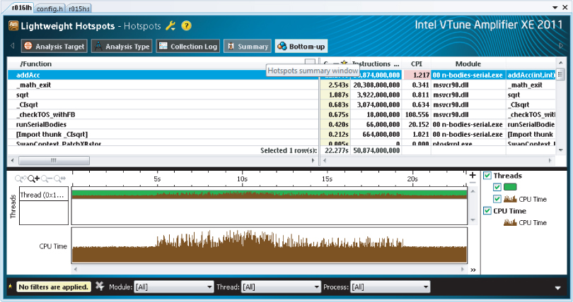
Any optimization effort should focus on parts of the code with the most intense CPU activity. Figure 14.2 shows the results of an Amplifier XE Hotspot analysis session. The main hotspot consuming most of the CPU activity is the addAcc() function. You can try this out for yourself in Activity 14-1.

Figure 14.2 The Hotspot analysis shown in Amplifier XE

The fundamental problem of an n-bodies simulation is the number of calculations that need to be performed.

You can easily see how the number of calculations needed rapidly grows by looking at the serial version of the n-bodies code. All the bodies in the simulation are held in the array body. The size of the array BODYMAX is the same as the number of bodies you are simulating. Each element of the array body holds a BODYTYPE structure, which stores the position, velocity, acceleration, and mass of the body:

struct BODYTYPE {
    double pos[NUMDIMENSIONS];
    double vel[NUMDIMENSIONS];
    double acc[NUMDIMENSIONS];
    double mass;
// …
};
BODYTYPE body[BODYMAX];

To perform a brute-force simulation, the interaction between every body is calculated in a triple-nested loop within the function runSerialBodies. At the innermost level of the loop, the function addAcc combines the acceleration of the two bodies. Once all the accelerations have been calculated, the function ApplyAccelerationsAndAdvanceBodies applies the new accelerations to each body in the simulation:

void runSerialBodies(int n)
{
  // Run the simulation over a fixed range of time steps
  for (double s = 0.; s < STEPLIMIT; s += TIMESTEP)
  {
    int i, j;
    // Compute the accelerations of the bodies
    for (i = 0; i < n - 1; ++i)
      for (j = i + 1; j < n; ++j)
        addAcc(i, j);
    // apply new accelerations
    ApplyAccelerationsAndAdvanceBodies(n);
    }
}

In Dr. Golanski's work, the simulation time was reduced by using a hashed tree-based n-bodies simulation using a modified Barnes-Hut algorithm.¹

## TODO: EDIT next set of lines according to OS
#include windows.inc
include linux.inc

$ source /opt/intel/bin/compilervars.sh intel64

make clean
make 14-1

nmake clean
nmake 14-1

Running with 1024 bodies
Running Serial  Release version
Body initialization took  0.0000 seconds
Simulation took 19.218 seconds
Number of Calculations: 524299776

amplxe-gui

Using a Tree-Based N-Bodies Simulation

The trick in the Barnes-Hut algorithm is to group together clusters of particles and treat them as a single body. When calculating the effect of such a group on a nearby particle, the distance of the particle to the group is first examined. If a group is greater than a certain distance away, the combined mass of the group is used rather than the mass of the individual particles within the group. Because of this grouping, the time taken to calculate the effect of particles on each other is reduced significantly.

The first stage in building up the simulation model is to create a single cube that represents the entire space of the environment. As the model is populated, this cube is partitioned into smaller cubes. Each cube can contain at most only one particle, so when two particles would occupy the same cube, the cube is split into sub-cubes so that each particle can be in its own cube. Figure 14.3 shows how this cube division takes place:

• The first particle is placed into the single cube. This is represented by the head node in the octree.
• Introducing a second particle causes the head cell to be split into eight, the two particles now being stored in the second- level of the tree.
• Additional particles are placed in the new leaf(s). When two particles end up being in the same cube, the cube is split into a further eight cuboids.
• A fully constructed tree consists of nodes and leaf(s). Only a leaf can contain a particle.

Figure 14.3 The entire environment to be simulated is represented as a set of cubes, which is stored as an octree

The collection of nested cubes is stored in an octree. An octree works the same way as a binary tree, except that each node has eight children rather than the usual two. The octree is traversed recursively using standard linked-list techniques. The mass and center of mass is calculated for every node in the tree.

The following code snippet shows the three structures that are used to store the octree — NODE, NODES, and TREE. The width of the octree is determined by TREE_WIDTH, which is defined to have the value 8.

struct NODE
{
       int Id;
       BODYTYPE * pCell;
       NODES *  pNodes;
       MINMAX MinMax;
       NODE * pNext; // used in linked list to all siblings
       NODE * pChild; // used in linked list to all children
       double CentreOfMass[NUMDIMENSIONS];
       double Mass;
};

struct NODES
{
       NODE Nodes[TREE_WIDTH];
}; 

struct TREE
{
       int NumNodes; // this includes number of leafs
       int NumLeafs;
       NODE Head;
}

Using a Hashed Octree

One way to implement the octree is to use linked lists, where each node of the linked list points to eight sub-children. Tree traversal using linked lists is expensive. Algorithms that use pointer-chasing techniques often suffer from poor performance due to inefficient use of memory. By using a hash-based algorithm rather than a linked list to store the tree, the traversal and manipulation of the tree is significantly reduced.

Dr. Golanski used a hash-based algorithm in which the xyz coordinates of the particle are used to construct a hash key, as described by Warren and Salmon.² Where the hash key is calculated to be the same for two different particles, the values are chained together under the same key. For example, in Figure 14.4(a) the bottom hash table entry has two additional entries (Bin 1 and Bin 2) that are daisy-chained to the #2249 hash.

Figure 14.4 Tree traversal and hash generation

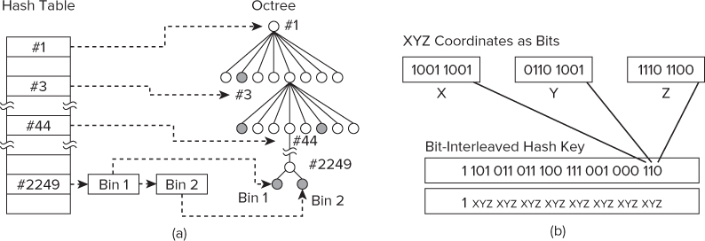
In the n-bodies simulation code, the HASHTABLE structure is used to hold the hash table. Each entry of the hash table is stored in the Data array, with the size of the array being controlled by the MAXKEYS:

struct HASHTABLE
{
       unsigned int NumNodes;
       unsigned int NumLeafs;
       unsigned int NumChainedLeafs;
       QUEUE SortedList;

       NODE Data[MAXKEYS];

};

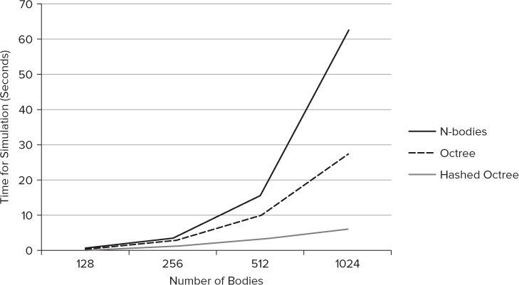
Implementing the simulation using a hashed octree resulted in a further improvement on the time taken for each simulation when using the same hardware. Figure 14.5 shows how the changes in the n-bodies algorithm affect the simulation time. In the traditional n-bodies solution, the time taken in the simulation rises very sharply as new bodies are introduced. The most favorable algorithm is the hashed octree, which produces a very manageable rate of rise.

Figure 14.5 Significant performance improvements can be made by changing the heuristics of the application

Architectural Tuning

Once you have suitably tuned the heuristics of the application, it's time to turn your attention to the architectural bottlenecks. Amplifier XE is used to perform the architectural analysis. A number of predefined analysis types are available for architectural analysis, including the following event-based types, which are targeted for Intel micro-architecture (see Chapter 12, “Event-Based Analysis with VTune Amplifier XE,” for more details):

• Lightweight Hotspots — Event-based sampling that captures the amount of time you spend in different parts of your code. This is different from the Hotspots analysis you have already used in Activities 14-1, 14-2, and 14-3 in that it does not collect any stack information.
• General Exploration — Event-based sampling collection that provides a wide spectrum of hardware-related performance metrics
• Memory Access — Event-based analysis that helps you understand where the memory access issues affect the performance of your application
• Bandwidth — Event-based analysis that helps you understand where the bandwidth issues affect the performance of your application
• Cycles and uOps — Event-based analysis that helps you understand where the uOp flow issues affect the performance of your application

As you become more experienced in architectural analysis, it is sometimes possible to guess what the likely bottlenecks will be. In the n-bodies code, the efficiency of the arithmetic operations, such as division, and how memory is used are at the top of the list of suspects you should investigate.

Within the identified hotspot function, there is code that contains several divisions:

  // compute the unit vector from j to i
  double ud[3];
  ud[0] = dx/dist;
  ud[1] = dy/dist;
  ud[2] = dz/dist;

This code can be rewritten to use a reciprocal, resulting in the compiler generating much faster code:

    // compute the unit vector from j to i
    double ud[3];
    double dd=1.0/dist;
    ud[0] = dx * dd;
    ud[1] = dy * dd;
    ud[2] = dz * dd;

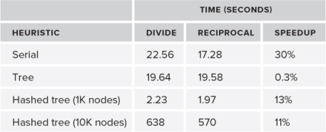
Table 14.1 shows the result of making such code changes on the different heuristics using the same hardware. The code was built using the Microsoft compiler. The number of particles used was 1024. Remember that it is better to look at the architectural bottlenecks after completing any heuristic optimization, not before. In the hashed tree solution — the code that has the most optimized heuristic — the speedup is 13 percent on a set of 1K particles and 11 percent on a set of 10K particles.

Table 14.1 Results of Optimizing Several Divisions

You often can make code, especially mathematical number-crunching code, more efficient by looking at how the calculations are done. By simply rearranging equations you can reduce the computational effort. The preceding divisional example is one such way of reducing the effort. In this example, a temporary variable was calculated and used three times. This idea can be further developed by precalculating parts of equations and carrying the results forward. Where several equations occur, make sure you are not calculating some part of the various equations more than once; again, use temporary variables. Often, array calculations can be broken down into several parts; this also increases the chances of their successful vectorization. All these approaches can reduce time even before other methods are considered.

Adding Parallelism

Once the serial version of the code is sufficiently well optimized, it's time to move on to making the code parallel. In the original research, the parallel algorithms were based on the suggestions made by Warren and Salmon. By splitting the sorted list of particles into groups, these groups can be simulated in parallel. Once the sorted particles are split into groups, a tree is created for each disjoint group — called local trees. Using a sorted list means that each group of particles is in spatially distinct parts of the cube. Where there is the possibility that a particle could sit in the node of an adjacent local tree, a copy of the node is held in both trees.

Identifying the Hotspot and Discovering the Calling Sequence

In the simulation, the same calculation is repeated thousands of times on the particles in the environment. Using Amplifier XE to identify the hotspots in the code shows that most of the time is spent adding the acceleration to the moving particles (refer to Figure 14.2).

Although the original research used MPI to implement parallelism, the steps that were undertaken to add parallelism are common to whatever language implementation is used.

The steps undertaken were as follows:

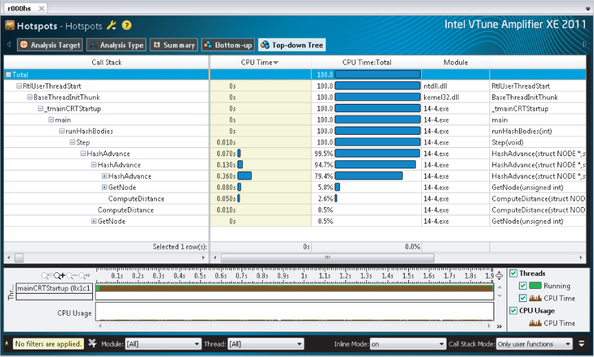
The most significant hotspot in the code is in the HashAdvance function. Normally, when applying parallelism, it is usual to add the parallel construct to one of the parent functions of the hotspot. As shown in Figure 14.6, the Step function looks like an ideal candidate. The function controls 99.5 percent of the CPU time.

Figure 14.6 Identifying the hotspot and call stack

Implementing Parallelism

As previously mentioned, the original implementation was done using MPI. Intel Parallel Composer provides a number of different ways of implementing parallelism, including OpenMP, Cilk Plus, and Threading Building Blocks. Cilk Plus is ideal for this kind of problem where load balancing is of upmost importance. Cilk Plus's task-stealing scheduler does a great job at load balancing and has an intuitive programming approach. Listing 14.1 shows how Cilk Plus can be applied to the problem.

Listing 14.1 shows how a for loop can be easily parallelized by using the cilk_for keyword at line 7. The code snippet is based on the Step() function found in Hash.cpp. The only other addition to the code was to include the statement #include <cilk/cilk.h> at the top of the file.

Listing 14.1: Introducing parallelism by replacing the for loop at line 7 with a cilk_for

1: // This code has known data race bugs and is used as an example
2: // to explain how to detect parallelization problems.
3: unsigned int stepcount;
4: void Step()
5: {
6:   // parallelize following loop using cilk_for in place of C for
7:   cilk_for(int i = 0; i < theTable.SortedList.Cursor; i++)
8:   {
9:     // declare and set hash table value
10:    unsigned int Hash = theTable.SortedList.List[i];
11:    if(Hash != 0)
12:    {
13:      // declare pointers to first & next nodes
14:      NODE *pNode = GetNode(Hash);
15:      NODE *pChain = pNode->pNext;
16:      // advance to next node and increment stepcount
17:      HashAdvance(pNode,GetNode(0));
18:      stepcount++;
19:      // while not end of list
20:      while(pChain)
21:      {
22:        // advance to next node
23:        HashAdvance(pChain, GetNode(0));
24:        pChain = pChain->pNext;
25:        stepcount++;
26:      }
27:    }
28:  }
29: }

code snippet chapter1414-1.cpp

Detecting Data Races and Other Potential Errors

Once parallelism has been introduced, there is always the risk that data races or other parallel-type errors have been accidentally introduced. Access within the threaded code to any global variable will cause problems. These problems can be detected using such tools as Intel Parallel Inspector (see Chapter 8, “Checking for Errors”).

A visual inspection of Listing 14.1 shows that the incrementing of the stepcount variable at line 18 and line 25 is likely to cause a data race. The variable is not declared with the scope of the parallelized loop, and can thus be accessed simultaneously by two or more worker threads. Using Intel Parallel Inspector XE will also show any problems.

The Intel Parallel Debug Extension (PDE) is another great way to detect data races. Figure 14.7 shows PDE detecting the data race. See Chapter 11, “Debugging Parallel Applications,” for more information on how to use PDE to detect data races.

Figure 14.7 Using Parallel Debugging Extension to detect data races

Correcting the Data Race

Cilk Plus provides a number of different ways to fix data races. The most obvious way is to restructure the code so that global variables are not needed. If you cannot restructure the code, protect access to the variable so that only one thread can modify it at any one time. By declaring the stepcount variable to be a cilk::reducer_opadd<unsigned int>, the Cilk Plus run time automatically ensures that no data race occurs. The Cilk Plus reducer does this by creating private copies or views of the variable within the parallel region, and then adding the private copies together (reducing the result) when leaving the parallel region.

inspxe-gui

Load Balancing

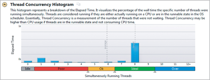
Once the n-bodies program is correctly running, verify that all the threads are employed usefully. The concurrency level is a measure of how parallel the program was running over its life. Figure 14.8 shows the concurrency view displayed in Parallel Amplifier XE. The application spends most of its time running all eight available cores.

Figure 14.8 Parallel Amplifier XE shows that the application has ideal thread concurrency

The Results

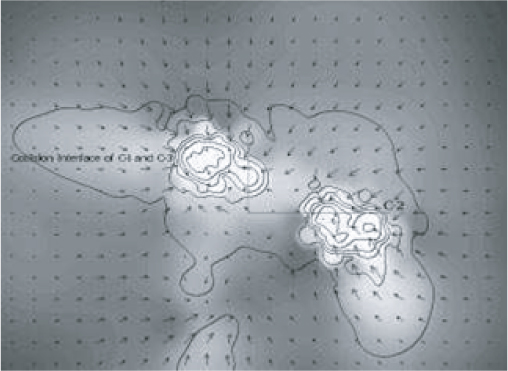
The original research work showed that adding coolant to the interstellar medium could result in a medium that was good enough to begin star formation. You can find a more detailed description of the results in the paper by Golanski and Woolfson. Figure 14.9 is a snapshot of the original simulation showing how introducing a coolant leads to the formation of two protostellar clouds, which eventually form dense cold clouds — the precursor to the formation of a star. The contours represent density; the shading, temperature; and the arrows, velocity and direction.

Figure 14.9 A snapshot of the original simulation

Summary

This chapter showed how you can look at the heuristics of a program to improve its efficiency — that is, reduce time. Simply changing the code can, in many instances, bring an instant speedup.

The performance was improved further by removing, where possible, architectural bottlenecks. The Intel VTune Amplifier XE was used to help in identifying and understanding the low-level bottlenecks.

The Intel Cilk Plus method of parallelization was then used in this case study to introduce parallel execution of the application, Cilk being ideal in this case due to its ease of use and ability to produce load-balanced code.

Chapter 15, “Parallel Track Fitting in the CERN Collider,” includes an example that shows how to use Intel Array Building Blocks (ArBB) to achieve parallelism on a collection of workstations. ArBB brings a flexible approach to parallelism, in which the runtime engine works alongside a just-in-time (JIT) compiler to produce optimized code, leading to software that can adapt itself to new generations of silicon as they become available.

¹ J. E. Barnes and P. Hut. 1986. A hierarchical O(N log N) force-calculation algorithm. Nature. 324, 446

² M. Warren and J. Salmon. 1993. A parallel hashed oct-tree N-body algorithm. Supercomputing ‘93 Proceedings. 12–21