![]()
Calculating Roots of Equations
Solving equations is one of the building blocks of many engineering and scientific algorithms. As financial algorithms become more sophisticated, there is a great need to calculate the results of equations in general. These results are frequently used in the analysis of investments and in new trading strategies. It is important not only to be able to solve equations but also to calculate the roots of such equations in an efficient way.
In this chapter you will learn some of the popular methods for calculating roots of equations. The coding recipes presented here cover different methods of calculating equation roots, along with explanations of how they work and when they should be used. Following are some of the topics covered in this chapter:
- Bisection method: a simple method that explores the change in signal around the root of equations; this method is easy to implement. You will learn the basics of the bisection method and how to code it in C++.
- Secant method: the secant method is an improvement over the bisection method, which tries to use the value of the function in the given range to guide the position of the new approximation of the root. The secant method can in many cases speed up the search for a root.
- Newton’s method: This method, sometimes also called the Newton/Raphson method, uses the derivative of a function as the guide for the search of the root for a given equation. Since the derivative determines the slope of the tangent to the function, its value can be used to calculate a new approximation. Successive values may converge to the desired solution, and an error parameter can be used to determine when to stop the process.
Create a class implementing the bisection method to find roots of equations.
Solution
Finding the roots of an equation is the process of determining any points for which the corresponding function is zero. During the development of computational mathematics, several methods have been devised to calculate roots of equations. This chapter covers a few of the most common of these methods.
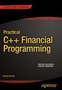
The bisection method tries to find the roots of equations by using a simple strategy: the idea is to look at the sign of the function at different points of the domain and use that information to decide if there is a root on that interval. For example, consider the function
f (x) = (x–1)3
Figure 9-1 displays the graph of this function in the interval -1 to 3.
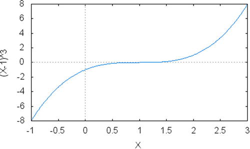
Figure 9-1. Function (x–1)3 in the interval -1 to 3
This is a function that has a root for the value x=1 and has two areas that have distinct signs: for values less than x=1 the sign is negative. For values greater than 1, the sign of the function is positive. If you want to determine the exact place where the function is equal to zero, you can start from an interval where the sign of the function is different (in this case you could use the interval -1 to 3) and look for the exact value where the function changes sign: that must be the location of one of the roots of the function.
![]() Note This argument works only when the function that you’re dealing with is continuous. That is, there is no point where the function suddenly jumps from one point to another, which would make the foregoing argument invalid. Continuous functions are differentiable in the range where they’re defined, so that is a way to know if a function is continuous. Most functions in economics, physics, and engineering have this property, so we assume that this is the case when the bisection method is applied.
Note This argument works only when the function that you’re dealing with is continuous. That is, there is no point where the function suddenly jumps from one point to another, which would make the foregoing argument invalid. Continuous functions are differentiable in the range where they’re defined, so that is a way to know if a function is continuous. Most functions in economics, physics, and engineering have this property, so we assume that this is the case when the bisection method is applied.
With this intuitive insight, the bisection method tries to employ a systematic approach to determine the range tested and the location where the change of sign occurs. Essentially, the method is to bisect the original range and determine if the subrange still has different signs.
For example, using the same function, consider that we take the original range between -1 and 2. The middle of this range is ½ and therefore the algorithm will check the sign of 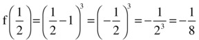 . Now, consider the sign of the two ending points of the initial range:
- f(–1) = (–1–1)3 = –8, therefore with a negative sign.
- f(2) = (2–1)3=13 = 1, therefore with a positive sign.
This means that between the values x = –1 and ![]() the sign is identical. On the other hand, between
the sign is identical. On the other hand, between ![]() and x = 2 the sign changes. Therefore, the root must be in the place where the sign changes, which is somewhere between ½ and 2.
and x = 2 the sign changes. Therefore, the root must be in the place where the sign changes, which is somewhere between ½ and 2.
Another iteration of this process will calculate the value of  , which has a positive sign. Since f (1/2) has a negative sign and f (2) has a positive sign, the change in sign must happen in the interval from
 ![]() to
to ![]() . This is easily observed to be true by checking the graph in Figure 9-1.
. This is easily observed to be true by checking the graph in Figure 9-1.
Notice that this process will systematically reduce the size of the range where we’re searching for a root of the equation. At each step we’re decreasing the range by a half, and getting closer to the location of the root. After a number of iterations you will get a value that is as close as needed from the true root. This algorithm therefore can stop whenever the size of the remaining range is less than the desired error. For example, if the range is less than 0.001, and your desired error is 0.01, then stop.
Using the process we just described, we can now describe the algorithm for bisection in the following way:
- Define an initial range (a,b) where you want to search for one or more roots of the equation.
- Calculate the values of f(a) and f(b).
- Determine the bisection point
 for the interval (a,b) and its corresponding function value f(c).
 - If the signs of f(a) and f(c) are different, (a,c) becomes the new range for the algorithm. Otherwise, the new range is defined as (c,b).
- If the new range has length less than the error (threshold) E, stop and report c as the solution. Otherwise, continue with step 1.
The preceding algorithm works in an iterative way, where the size of the range (a,b) is constantly reduced by half. Therefore, the number of steps it will perform is bounded by  . There is a trade-off between number of iterations and desired approximation, which means that if you want a very small error, more iterations will be necessary.
The procedure described has been coded as the part of the BisectionSolver class, which can be used to find roots of equations. The interesting characteristic of BisectionSolver is that it is a generic solver for any continuous function. You just need to pass the function as a parameter to the constructor of the class.
For this purpose, I created a class called MathFunction that will be useful not only here but also for other classes that use functions as parameters. The MathFunction class defines what is called a functional object, that is, an object that behaves like a function. This is important for our algorithms, because it allows one to use the object as if it were a function.
To create a functional object, you need a class that implements operator(), that is, the operator for function invocation. Moreover, I have defined the class MathFunction as a template class, so that you can pass the right return type when creating the concrete implementation. For example, you may want to define a MathFunction subclass that is defined for float values only. Or, conversely, you may have a function whose domain is the set of integers.
Finally, I want MathFunction to be just a root class, so that only concrete implementations can be instantiated. To make this possible, MathFunction is an abstract class, which is defined by using the =0 notation after the declaration of operator(). Concrete subclasses of this class need to provide a concrete implementation of this operator. The example code shows how this can be done.
class F1 : public MathFunction<double> {
public:
        virtual ~F1() {}
        virtual double operator()(double value);
};

double F1::operator ()(double x)
{
        return (x-1)*(x-1)*(x-1);
}
This is a definition for the example function f(x) = (x–1)^3.
The implementation of the function getRoot is straightforward. The function starts with the interval given as a parameter and halves it using the criteria defined by the bisection method.
Complete Code
//
// MathFunction.h

#ifndef MATHFUNCTION_H_
#define MATHFUNCTION_H_

template <class Res>
class MathFunction {
public:
        MathFunction();
        virtual ~MathFunction();
        virtual Res operator()(Res value) = 0;
};

#endif /* MATHFUNCTION_H_ */

//
// BisectionMethod.h

#ifndef BISECTIONMETHOD_H_
#define BISECTIONMETHOD_H_

template <class T>
class MathFunction;

class BisectionMethod {
public:
        BisectionMethod(MathFunction<double> &f);
        BisectionMethod(const BisectionMethod &p);
        ~BisectionMethod();
        BisectionMethod &operator=(const BisectionMethod &p);
        double getRoot(double x1, double x2);

private:
        MathFunction<double> &m_f;
        double m_error;
};

#endif /* BISECTIONMETHOD_H_ */

//
// BisectionMethod.cpp

#include "BisectionMethod.h"

#include "MathFunction.h"
#include <iostream>

using std::cout;
using std::endl;

namespace {
const double DEFAULT_ERROR = 0.001;
}

BisectionMethod::BisectionMethod(MathFunction<double> &f)
: m_f(f),
  m_error(DEFAULT_ERROR)
{
}

BisectionMethod::BisectionMethod(const BisectionMethod &p)
: m_f(p.m_f),
  m_error(p.m_error)
{
}

BisectionMethod::~BisectionMethod()
{
}

BisectionMethod &BisectionMethod::operator =(const BisectionMethod &p)
{
        if (this != &p)
        {
                m_f = p.m_f;
                m_error = p.m_error;
        }
        return *this;
}

double BisectionMethod::getRoot(double x1, double x2)
{
        double root = 0;
        while (std::abs(x1 - x2) > m_error)
        {
                double x3 = (x1 + x2) / 2;
                root = x3;
                if (m_f(x1) * m_f(x3) < 0)
                {
                        x2 = x3;
                }
                else
                {
                        x1 = x3;
                }
                if (m_f(x1) * m_f(x2) > 0)
                {
                        cout << " function does not converge "  << endl;
                        break;
                }
        }
        return root;
}

// ---- this is the implementation for an example function

namespace {

class F1 : public MathFunction<double> {
public:
        virtual ~F1();
        virtual double operator()(double value);
};

F1::~F1()
{
}

double F1::operator ()(double x)
{
        return (x-1)*(x-1)*(x-1);
}

}

int main()
{
        F1 f;
        BisectionMethod bm(f);
        cout << " the root of the function is " << bm.getRoot(-100, 100) << endl;
        return 0;
}
Running the Code
To run the code, along with the example provided, use a compiler such as gcc to generate the executable bisectionMethod. Then, you can run it to get results as follows:
./bisectionMethod
root is 0
root is 50
root is 25
root is 12.5
root is 6.25
root is 3.125
root is 1.5625
root is 0.78125
root is 1.17188
root is 0.976562
root is 1.07422
root is 1.02539
root is 1.00098
root is 0.98877
root is 0.994873
root is 0.997925
root is 0.999451
root is 1.00021
the root of the function is 1.00021
This shows the result of executing the bisection method on the function f(x) = (x–1)^3, starting with the interval -100 to 100. I showed the intermediate steps just for clarity.
Create a class to solve equations using the secant method.
Solution
In the previous programming recipe you learned about the bisection method for the solution of equations. You can find the roots of an equation through the decomposition of the domain into a set of ranges, each of which you can test for changes in sign. If the sign of the function is different from the sign at the end of the interval, then it is possible to find a point where this function changes from positive to negative, making it the root of the equation.
While the bisection method can find solutions to a large number of equations, it is not the fastest method for this purpose. One of the reasons is that it doesn’t use any of the properties of the function other than the sign at the extremes of its range. On the other hand, using additional information about the function values, for example, it would be possible, at least in principle, to achieve a faster convergence to the root of the function.
One of the ways to use the value of the function is contained in the algorithm called the secant method. The general idea of the secant method is to use the function value at the extremes of each interval as a way to approximate how close one is from the true root of the equation. In this way, it is possible to get closer to the root and reduce the number of iterations necessary to find the desired solution.
The secant of a function is the name given to the line connecting to points defined by that function. For example, given the function f(x) = x2 in the range 1 to 4, the secant to that function in the given range is the line segment connecting the points (1,1) and (4,16), since these are the two points defined by function. We can generalize this concept to any function that is continuous in a particular range.
The secant method uses information derived from the secant to the function to define the new segment to be explored. To do this, the method calculates the point of intersection of the secant with the x-axis, and uses that point to define the new segment. This is possible whenever the sign of the points at the beginning and end of a range are different, because in that case the secant will intercept with the x-axis. As you may remember from the previous recipe, this is similar to the criterion used by the bisection method, with the difference that bisection uses the midpoint, instead of a point based on the secant of the function.
As an example of how this works in practice, consider the same function used in the section “Bisection Method”: f(x) = (x–1)3, in the range -1 to 2. In this case, we can calculate the values of f(–1) = –8 and f(2) = 1, which have different signs. We can, based on that information, use the secant to the function on this interval to find an intersection with the x-axis. The line segment we want to use is, therefore, connecting the points (–1,–8) and (2,1).
With a little of algebra, you will find that the slope of this line is
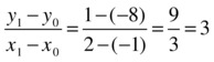
And, since it is known that the point (x1,y1) = (2,1) is touched, the secant line is given by:
h (x) = y1+ 3 (x–x1) = 1 + 3 (x–2)
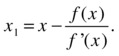
Now, the intersection point with the x-axis can be calculated using this equation and the fact that h(x) = 0 at the intersection (see Figure 9-2)
0=1+3x–6=–5+3x
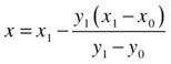
This means that ![]() is the intersection point between the secant and the x-axis. You can easily see, as shown in Figure 9-2, that the intersection of the secant with the x-axis is a point (let’s call it x2) that is one step closer to the root of the equation. This process can be repeated with the new interval defined by x0 and x2, until the root of the equation is approximated within a small error (which can be predefined by the algorithm).
is the intersection point between the secant and the x-axis. You can easily see, as shown in Figure 9-2, that the intersection of the secant with the x-axis is a point (let’s call it x2) that is one step closer to the root of the equation. This process can be repeated with the new interval defined by x0 and x2, until the root of the equation is approximated within a small error (which can be predefined by the algorithm).
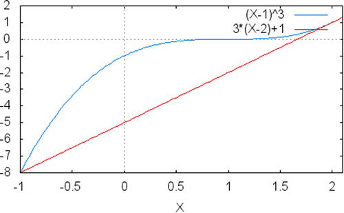
Figure 9-2. The original function (x–1)3 and its secant in the interval -1 to 2
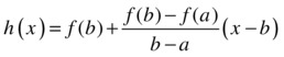
Generalizing the h(x)= equation shown just a bit earlier, the equation for the secant can be denoted as:
When this equation intercepts with the line y=0, we have
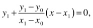
which yields the result
With this equation, we can calculate the new point x that will be used at the next step of the algorithm. Summarizing the steps described, the secant method for finding roots of equations can be described in the following way:
- Define an initial range (a,b) where you want to search for one or more roots of the equation.
- Calculate the values of f(a) and f(b).
- Determine the secant line using the equation
- Using this equation, find the intersection point
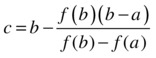
- If the difference |c – b| has length less than the error (threshold) E, stop and report c as the solution. Otherwise, continue with step 1.
It has been observed that for some functions this algorithm converges to a solution more quickly than the bisection algorithm. This happens because the secant uses information that is already available with the function, which happens to make the intermediate point closer to the real solution.
You can find an implementation of the algorithm discussed in the SecantSolver class. The design of this class is similar to BisectionSolver, since the problem discussed is the same. The main change is the use of a different middle point selection procedure, which makes this algorithm a little different from that presented in BisectionSolver.
Complete Code
// SecantMethod.h
//

#ifndef SECANTMETHOD_H_
#define SECANTMETHOD_H_

template <class T>
class MathFunction;

class SecantMethod {
public:
        SecantMethod(MathFunction<double> &f);
        SecantMethod(const SecantMethod &p);
        SecantMethod &operator=(const SecantMethod &p);
        ~SecantMethod();

        double getRoot(double x1, double x2);
private:
        MathFunction<double> &m_f;
        double m_error;
};

#endif /* SECANTMETHOD_H_ */
// SecantMethod.cpp
//

#include "SecantMethod.h"

#include "MathFunction.h"
#include <iostream>

using std::cout;
using std::endl;

namespace {
const double DEFAULT_ERROR = 0.001;
}

SecantMethod::SecantMethod(MathFunction<double> &f)
: m_f(f),
  m_error(DEFAULT_ERROR)
{
}

SecantMethod::SecantMethod(const SecantMethod &p)
: m_f(p.m_f),
  m_error(p.m_error)
{
}

SecantMethod::~SecantMethod()
{
}

SecantMethod &SecantMethod::operator=(const SecantMethod &p)
{
        if (this != &p)
        {
                m_f = p.m_f;
                m_error = p.m_error;
        }
        return *this;
}

double SecantMethod::getRoot(double x1, double x2)
{
        double root = 0;
    double fa = m_f(a);
    double fb = m_f(b);
    double c = 0, fc = 0;
        do
        {
        c = b - fb*(b-a)/(fb-fa);
                root = c;
        fc = m_f(c);

        cout << "-> " << c << " " << fc << " " << endl; // this line just for demonstration

        a  = b;
        fa = fb;
        b  = c;
        fb = fc;
    }
    while (std::abs(a - b) > m_error);
        return root;
}

// ---- this is the implementation for an example function

namespace {

class F2 : public MathFunction<double> {
public:
        virtual ~F2();
        virtual double operator()(double value);
};

F2::~F2()
{
}

double F2::operator ()(double x)
{
        return (x-1)*(x-1)*(x-1);
}

}

int main()
{
        F2 f;
        SecantMethod sm(f);
        double root = sm.getRoot(-10, 10);
        cout << " the root of the function is " << root << endl;
        return 0;
}
Running the Code
After compiling the code presented previously, you can run it and get the following results, which show the solution for the sample equation f(x) = (x–1)3:
./secantMethod
-> 2.92233 7.10369
-> 2.85268 6.35922
-> 2.25777 1.98976
-> 1.98685 0.96108
-> 1.73375 0.395035
-> 1.5571 0.172905
-> 1.41961 0.0738799
-> 1.31702 0.0318621
-> 1.23923 0.0136922
-> 1.18062 0.00589209
-> 1.13634 0.00253417
-> 1.10292 0.00109016
-> 1.07769 0.000468932
-> 1.05865 0.000201717
-> 1.04427 8.67704e-05
-> 1.03342 3.73252e-05
-> 1.02523 1.60558e-05
-> 1.01904 6.90655e-06
-> 1.01438 2.97092e-06
-> 1.01085 1.27797e-06
-> 1.00819 5.49731e-07
-> 1.00618 2.36472e-07
-> 1.00467 1.01721e-07
-> 1.00352 4.37562e-08
-> 1.00266 1.88221e-08
 the root of the function is 1.00266
Create a C++ class to implement Newton’s method for calculating roots of equations.
Solution
As you have seen in the last few sections, it is possible to find solutions for a large number of equations by just using a bisection method. You can also try to improve the rate of convergence using additional information from the function, in such a way that the secant of the function is used in the desired interval. Taking this idea one step further, you will arrive at one of the most used methods for solving equations, which is attributed to Isaac Newton.
Newton’s method for finding roots of equations uses the derivative of the function as a first approximation to the location of the root. Similar to the previous two methods you have seen, the process is iterative, and at each step you can get closer to the real root of the equation. At the end, you will have a solution that is within a very small error, which can be determined before the algorithm starts.
To understand how the method works, consider again the function f(x) = (x–1)3, which we have been using as an example. The derivative of this function can be easily calculated, since this is a polynomial, and is given by f’(x) = 3(x–1)2. Now, suppose that you start with an initial guess of what the root value might be (if there is no guess, consider a random value as the starting point). Call that initial guess x0. At that point, we can calculate two values, f(x0) and f'(x0).
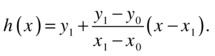
In Figure 9-3 you will find a plot of the function and its tangent at point x0 = 0 for the example function given previously. At that point, the value of f(x0) = f(0) = –1 and the value of f'(x0) = f'(0) = 3. Since the derivative of the function at a particular point represents the slope of the tangent to the curve at that point, we can calculate a point x1, which is determined by the line that is tangent with the given equation using the following formula:
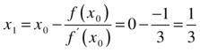
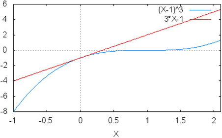
Figure 9-3. The example function f(x) = (x–1)3 and its tangent at point x0 = 0. You may notice that the tangent intersects the x-axis at point  . This is the first step in finding the root for the given function using Newton's method
Once the intersection of the x-axis and the tangent has been found, you have a new starting point for the determination of the root for the given equation. Notice that, each time a new point is found, the algorithm gets a little closer to the desired point, although it may take a few iterations to achieve the desired precision. As in the previous two cases, you can determine the precision as a parameter to the algorithm, and stop the computation once the difference between two successive approximations is less than the given parameter. This shows that the solution is converging to a point where the root is located.
In summary, Newton’s method works by successively finding points that are determined by the tangent to the function. As you get closer to the root, the difference between the intersection of the tangent with the x-axis will get smaller. The stopping condition is that difference between the last and the current values is less than a given parameter.
Based on the previous information, the algorithm for Newton’s method can be given as follows:
- Define an initial value x, from which you want to search for one or more roots of the equation.
- Given the input function f(x), determine the derivative of function f'(x).
- Calculate the values of f(x) and f'(x) for the desired value.
- Using the value f'(x) as the slope of the tangent at the point x, calculate a new point x1 using the following equation:
- Calculate the difference between x and x1 as e = |x–x1|.
- If the value of e is less than the input error (threshold) E, stop and report x as the solution. Otherwise, rename x1 to x and continue with step 1.
The fact that Newton’s method depends not only on the function but also on its derivative can be seen as an advantage as well as a disadvantage. Sometimes it is very easy to compute the derivative of a function, such as for polynomial and common trigonometric functions, but that is not always the case. However, the greatest advantage of Newton’s method is that, unlike the bisection and secant methods, it works even when there is no difference in function sign.
Consider, for example, the function f(x) = (x–1)2. Its graph is shown in Figure 9-4. Notice that, unlike other functions that you saw in this chapter, there is no place where it changes sign. Therefore, without some changes to the bisection method, it is not possible to find a root in this case. On the other hand, the function clearly has a derivative, being differentiable everywhere, and this makes it possible to find the root using Newton’s method.
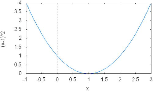
Figure 9-4. A continuous, quadratic function (x–1)2 that never changes sign but has a single root at x = 1
A small issue that we need to consider when using Newton’s method is the possibility that the derivative is zero at some point. If that is the case, then the next point is undefined, since a division by zero is not permitted. This difficulty can be avoided, however, if the algorithm adds a small value to the current point as a way to avoid the issue. More sophisticated techniques to solve this problem exist, however, as the reader will be able to find in one of the many existing books on the topic of numerical algorithms.
The previous algorithm was coded in C++ in the class NewtonMethod, which provides the necessary support for all the steps described. The design of the class is very similar to what you saw for the bisection method. Unlike the bisection method and the secant method, however, NewtonMethod depends not only on the function but also on its derivative. That’s why in the example code you will see a reference to two functions: F3 and DF3. They are necessary so that the NewtonMethod class knows how to find the value of the function and its derivative.
Complete Code
//
// NewtonMethod.h

#ifndef NEWTONMETHOD_H_
#define NEWTONMETHOD_H_

template <typename T>
class MathFunction;

class NewtonMethod {
public:
        NewtonMethod(MathFunction<double> &f, MathFunction<double> &derivative);
        NewtonMethod(const NewtonMethod &p);
        virtual ~NewtonMethod();
        NewtonMethod &operator=(const NewtonMethod &p);

        double getRoot(double initialValue);
private:
        MathFunction<double> &m_f;
        MathFunction<double> &m_derivative;
        double m_error;
};

#endif /* NEWTONMETHOD_H_ */

//
// NewtonMethod.cpp

#include "NewtonMethod.h"

#include "MathFunction.h"

#include <iostream>

using std::endl;
using std::cout;

namespace {
const double DEFAULT_ERROR = 0.001;
}

NewtonMethod::NewtonMethod(MathFunction<double> &f, MathFunction<double> &derivative)
: m_f(f),
  m_derivative(derivative),
  m_error(DEFAULT_ERROR)
{
}

NewtonMethod::NewtonMethod(const NewtonMethod &p)
: m_f(p.m_f),
  m_derivative(p.m_derivative),
  m_error(p.m_error)
{
}

NewtonMethod::~NewtonMethod()
{
}

NewtonMethod &NewtonMethod::operator=(const NewtonMethod &p)
{
        if (this != &p)
        {
                m_f = p.m_f;
                m_derivative = p.m_derivative;
                m_error = p.m_error;
        }
        return *this;
}

double NewtonMethod::getRoot(double x0)
{

    double x1 = x0;
    do
    {
        x0 = x1;
        cout << " x0 is " << x0 << endl;  // this line just for demonstration
        double d = m_derivative(x0);
        double y = m_f(x0);
        x1 = x0 - y / d;
    }
    while (std::abs(x0 - x1) > m_error);

    return x1;

}

// ---- this is the implementation for an example function and its derivative

namespace {

class F3 : public MathFunction<double> {
public:
        virtual ~F3();
        virtual double operator()(double value);
};

F3::~F3()
{
}

double F3::operator ()(double x)
{
        return (x-1)*(x-1)*(x-1);
}

class DF3 : public MathFunction<double> {
public:
        virtual ~DF3();
        virtual double operator()(double value);
};

// represents the derivative of F3
DF3::~DF3()
{
}

double DF3::operator ()(double x)
{
        return 3*(x-1)*(x-1);
}

}

int main()
{
        F3 f;
        DF3 df;
        NewtonMethod nm(f, df);
        cout << " the root of the function is " << nm.getRoot(100) << endl;
        return 0;
}
Running the Code
The code can be compiled and linked using a compiler such as gcc on UNIX. To run the resulting program and see its associated results, use the following command line:
./newtonMethod
x0 is 100
 x0 is 67
 x0 is 45
 x0 is 30.3333
 x0 is 20.5556
 x0 is 14.037
 x0 is 9.69136
 x0 is 6.79424
 x0 is 4.86283
 x0 is 3.57522
 x0 is 2.71681
 x0 is 2.14454
 x0 is 1.76303
 x0 is 1.50868
 x0 is 1.33912
 x0 is 1.22608
 x0 is 1.15072
 x0 is 1.10048
 x0 is 1.06699
 x0 is 1.04466
 x0 is 1.02977
 x0 is 1.01985
 x0 is 1.01323
 x0 is 1.00882
 x0 is 1.00588
 x0 is 1.00392
 x0 is 1.00261
the root of the function is 1.00174
The algorithm executes the steps for Newton’s method for the function f(x) = (x–1)3. Notice that even when starting from a distant value of 100, the algorithm converged to the solution 1.0 within the required error.
Conclusion
In this chapter, you have seen a few recipes that deal with the search for roots of equations. This is a topic that is frequently useful in the solutions of equations appearing in financial engineering. Algorithms for trading and for investment analysis frequently require the solution of equations, which makes it necessary to find efficient techniques for the determination of equation roots.
In this chapter, I presented some of the most common techniques for the solution of equations that appear in finance. More specialized algorithms exist, however, and you can use the numerical methods literature as a starting point to explore the most recent methods.
The programming recipes in this chapter show, initially, how to compute the root solution for equations using the bisection method. With the bisection algorithm, the desired range of the domain is divided evenly, and at each step possible location of the root is approximated with higher accuracy. Due to the sign of the function in each end point of the range, it is possible to detect if a root of the equation is contained in that range. At the end of the procedure, one can determine within a small margin of error the location where the equation becomes zero.
Next, you have seen a programming recipe for the secant method to solve equations. The method is based on the use of the secant line to the function in the interval that is being considered. When the secant intersects the x-axis, the new point is usually closer to the root of the equation. Performing several iterations of this procedure, it is possible to find the desired solution in less time than needed by the bisection method.
You have also learned about the most popular method for the determination of equation root, known as Newton’s method. With this algorithm, a solution can be found through the use of the tangent to the function at a given point. Since the derivative of a function gives the slope of the function at each point, it is possible to use the derivative to find a reasonable approximation. As the algorithm iterates through successive points, the approximation gets better. As with other methods, the algorithm is generally stopped when a preset maximum error is achieved.
In the next chapter I will talk about another important computational tool that is heavily used in financial algorithms: numerical integration. With algorithms for numerical integration it is possible to find solutions for several difficult problems with a high degree of precision. You will also see how to implement these techniques using C++.