![]()
Interpolation
Interpolation is a commonly used technique that approximates a mathematical function, based on a set of points given as input. Fast interpolation is the secret for high-performance algorithms in several areas of financial engineering. This chapter shows you a few programming recipes that cover some of the most common aspects of interpolation techniques, along with their efficient implementation in C++. You will explore the main procedures used in applications and see examples of how they work in practice.
Here are some of the topics covered in this chapter.
- Interpolation examples: a brief discussion of examples that show the effectiveness of using interpolation in financial problems.
- Linear Interpolation: one of the simplest interpolation techniques, linear interpolation uses linear functions, which can be represented as line segments. The quick nature of this technique makes it one of the most used forms of interpolation for functions that are hard to compute.
- Polynomial interpolation: if smooth transitions between different parts of the function are required, then it not possible to use a linear interpolation directly. Polynomial interpolation allows the use of a single function that approximates all of the given points through a high-degree polynomial. You will see how to construct this polynomial and return the desired function for each value of the domain.
Write a solution, along with C++ code, for the problem of interpolating a given set of data points using linear approximations.
Solution
Interpolation is the process of finding a function (or set of functions) that can be used to approximate an unknown function, as determined by a given set of points. The input for this process is therefore the points you would like to interpolate. The result is a general function that can be used to compute the unknown values for points outside the input set.
For example, suppose that you are given a time series composed of a set of observations. It is frequently desirable to find a function that generated those points. This estimation of the unknown function may also be used to calculate the corresponding value for a required time instant.
Interpolation has been used in several areas of science and engineering as a way to approximate functions. This may be necessary either because the original function is truly unknown (for example, in the case of empirical processes) or because such a function is very difficult to calculate exactly. In finance, interpolation also plays an important role, frequently as part of more complex algorithms. In the case of a financial time series, for example, interpolation allows practitioners to calculate values for a time series that are difficult to compute, while using only an approximation for the unknown function. Moreover, in some of these applications, interpolation can also be used as a way to forecast values, at least for short periods of time. In this role, it can also be used as a simple forecasting component of trading algorithms.
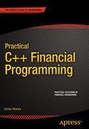
In this section, you will see how to perform interpolation using linear functions. This is the simplest way to provide the interpolation of a set of points, since it requires only two points at a time in order to directly connect input values. For example, suppose that you’re give a set of points, as displayed in Figure 8-1:
y1 = (10,0.6), y2 = (20,0.11), y3 = (30,1.1), y4 = (40,1.62), y5 = (49,1.4).
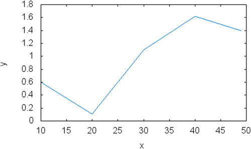
Figure 8-1. Interpolation graph for points in the first example
The points don’t need to be evenly spaced, although that might work better when a linear interpolation is desired. Using these points one can visualize a simple way to interpolate values. The strategy for creating an interpolation is to sort the input points based on their first dimension (the x axis on Figure 8-1) and join with a line the two points that are right before and after the desired value of x. The interpolation is then given by the formula in Step 4 of the list following Figure 8-1.
The algorithm for the linear interpolation of a set of points can, therefore, be summarized in the following steps:
- Read the input values (x[i],y[i]) and the desired coordinate value x.
- Sort the input in increasing order of the first coordinate (x[i]).
- Calculate the first pair of points (x[i],y[i]), (x[j],y[j]) such that j=i+1 and x is within x[i] and x[j].
- Use the following equation to determine the value of y corresponding to x:

You can easily implement this algorithm in C++ so that the function is computed for each value of x. I present the LinearInterpolation as the main class responsible for storing the necessary data as well as calculating points using this interpolation technique.
The constructors for this class are generic to reduce any overhead for the creation of new objects. The class provides the setPoints member function as a way to define the known points of the interpolation. This member function retains the values passed as a parameter. It also makes sure that the points are stored in the order of increasing x values. This is done using a simple algorithm that sorts the x values (the standard function std::sort is used for this purpose).
//
//  LinearInterpolation.h

#ifndef __FinancialSamples__LinearInterpolation__
#define __FinancialSamples__LinearInterpolation__

#include <vector>

class LinearInterpolation {
public:
    LinearInterpolation();
    LinearInterpolation(const LinearInterpolation &p);
    ~LinearInterpolation();
    LinearInterpolation &operator=(const LinearInterpolation &p);
    void setPoints(const std::vector<double> &xpoints, const std::vector<double> &ypoints);
    double getValue(double x);
private:
    std::vector<double> m_x;
    std::vector<double> m_y;
};

#endif /* defined(__FinancialSamples__LinearInterpolation__) */

//
//  LinearInterpolation.cpp

#include "LinearInterpolation.h"

LinearInterpolation::LinearInterpolation()
: m_x(),
  m_y()
{
}

LinearInterpolation::LinearInterpolation(const LinearInterpolation &p)
: m_x(p.m_x),
  m_y(p.m_y)
{
}

LinearInterpolation::~LinearInterpolation()
{
}

LinearInterpolation &LinearInterpolation::operator=(const LinearInterpolation &p)
{
    if (this != &p)
    {
        m_x = p.m_x;
        m_y = p.m_y;
    }
    return *this;
}

void LinearInterpolation::setPoints(const std::vector<double> &xpoints,
                                    const std::vector<double> &ypoints)
{
    m_x = xpoints;
    m_y = ypoints;

    // update points to become sorted on x axis.
    std::sort(m_x.begin(), m_x.end());
    for (int i=0; i<m_x.size(); ++i)
    {
        for (int j=0; j<m_x.size(); ++j)
        {
            if (m_x[i] == xpoints[j])
            {
                m_y[i] = ypoints[j];
                break;
            }
        }
    }

}

double LinearInterpolation::getValue(double x)
{

    double x0=0, y0=0, x1=0, y1=0;
    if (x < m_x[0] || x > m_x[m_x.size()-1])
    {
        return 0; // outside of domain
    }

    for (int i=0; i<m_x.size(); ++i)
    {
        if (m_x[i] < x)
        {
            x0 = m_x[i];
            y0 = m_y[i];
        }
        else if (m_x[i] >= x)
        {
            x1 = m_x[i];
            y1 = m_y[i];
            break;
        }
    }

    return y0 * (x-x1)/(x0-x1) +  y1 * (x-x0)/(x1-x0);
}

int main()
{
    double xi = 0;
    double yi = 0;
    vector<double> xvals;
    vector<double> yvals;
    while (cin >> xi)
    {
        if (xi == -1)
        {
            break;
        }
        xvals.push_back(xi);
        cin >> yi;
        yvals.push_back(yi);
    }
    double x = 0;
    cin >> x;
    LinearInterpolation li;
    li.setPoints(xvals, yvals);
    double y = li.getValue(x);
    cout << "interpolation result for value " << x << " is " << y << endl;
    return 0;
}
Running the Code
For example, consider again the points in the example shown in Figure 8-1. To calculate a linear interpolation for value 27, you need to execute the application and enter the following data:
./linearInterpolation
10 0.6
20 0.11
30 1.1
40 1.62
49 1.4
-1
27
interpolation result for value 27 is 0.803
Construct a polynomial interpolation for a given set of points in C++.
Solution
In the previous recipe, you saw how data points may be used to interpolate values in a continuous interval, through the use of piecewise linear equations. However, while it is possible to use linear interpolation in a large number of practical situations, the problem with this type of approximation is that the resulting curve is non-smooth. This means that it contains inflection points that mark transitions in the function, exactly at the interception of the different lines. In mathematical terms, it is said that such functions are non-differentiable because of this sudden transition. Such perceptible changes are undesired in some applications, and you may want to interpolate the values in such a way that the transition between observed points is seamless.
To avoid the described problems with the use of linear interpolation, a more sophisticated scheme may be employed, which uses higher-degree polynomials to smooth out the transitions. What is more important, a single polynomial found using this method can be used to interpolate all given data points at the same time. The result of this type of interpolation is that you just need a single polynomial equation to generate values for any desired input.
Polynomial interpolation is based on the mathematical fact that, given a polynomial with a high enough degree, you can find a corresponding polynomial function that passes through the exact points that are provided as input. This is guaranteed due to some well-known algebraic properties of polynomials. For example, suppose that we’re given the sequence of points that follow (these are the same points used in the previous example for linear interpolation):
y1 = (10,0.6), y2 = (20,0.11), y3 = (30,1.1), y4 = (40,1.62), y5 = (49,1.4).
A polynomial interpolation algorithm would return a value based on a polynomial defined by a set of coefficients. Using that information you can calculate any intermediate point, or even points that are outside the given range of observations, since polynomials are typically defined for any real number. You can also use the calculated polynomial to plot the values of the interpolating function, as you see in Figure 8-2.
Figure 8-2. A polynomial function to interpolate values using a small number of observations: notice how the polynomial function is smooth, unlike the solution in Figure 8-1, which uses line segments
The technique used here to solve this polynomial interpolation problem is called Lagrange’s interpolation algorithm. Using Lagrange’s interpolation method, for each sequence of n+1 points (xi,yi), you can create a polynomial that has degree n and passes through these points. Using the points given as input, the general formula for the coefficients of the polynomial is given by
![]()
Notice that this function skips the value of xk to avoid zero terms in the numerator and denominator. Now, the complete polynomial representation for interpolating the input values xk can be written using the coefficients Lk(x).
![]()
This is a function that can be used to provide the interpolation of any value, given the n+1 input observations (xi, yi). The proof for this formula is beyond our goals in this section, but notice that when the input value x is one of the known xi, then it will have a component x – xi that will result in zero in all cases, but for Li(x). In that case, however, the numerator is the same as the denominator, which results in the value 1. Therefore, for these values the solution is just yi as expected.
Using this polynomial function, we can create a C++ class that implements the interpolation mechanism through the simulation of the desired polynomial. This is achieved using the class PolynomialInterpolation. The class has a design similar to LinearInterpolation, storing the x and y values that are passed in the setPoints member function. Using that information, PolynomialInterpolation is able to perform the necessary calculations based on the initial points.
The real work is of calculating the polynomial interpolation is performed in the getValue member function, which is reproduced as follows:
double PolynomialInterpolation::getPolynomial(double x)
{
    double polynomialValue = 0;

    for (size_t i=0; i<m_x.size(); ++i)
    {

        // compute the numerator
        double num = 1;
        for (size_t j=0; j<m_x.size(); ++j)
        {
            if (j!=i)
            {
                num *= x - m_x[j];
            }
        }

        // compute the denominator
        double den = 1;
        for (size_t j=0; j<m_x.size(); ++j)
        {
            if (j!=i)
            {
                den *= m_x[i] - m_x[j];
            }
        }

        // value for i-th term
        polynomialValue += m_y[i] * (num/den);
    }

    return polynomialValue;
}
The calculation is done in an iterative way, where at each step of the for loop one of the polynomials Lk(x) is computed and added to the local variable polynomialValue. The internal part of the loop can be divided into three parts. In the first part, the numerator is calculated as a result of multiplying all of the terms x – xj, something that is not necessary when i = j. The second part is the calculation of the denominator, which is very similar to the first step, as you can confirm looking at the original formula. The values of the denominator are stored in the local variable den. The third step consists of multiplying the value of y by the fraction defined by the numerator and denominator that were computed in the previous two steps.
The complexity of the algorithm previously described is dependent on the given input. The more input values you provide, the longer this algorithm will take. The variation in time is quadratic with the number of input values, since for each value we need to perform a for loop inside a second loop, and each such loop runs a number of times equal to the number of points used. In terms of computational complexity, this is said to have a time complexity of O(n2).
//
//
//  PolymonialInterpolation.h

#ifndef __FinancialSamples__PolymonialInterpolation__
#define __FinancialSamples__PolymonialInterpolation__

#include <vector>

class PolynomialInterpolation {
public:
    PolynomialInterpolation();
    PolynomialInterpolation(const PolynomialInterpolation &p);
    ~PolynomialInterpolation();
    PolynomialInterpolation &operator=(const PolynomialInterpolation &);
    void setPoints(const std::vector<double> &x, const std::vector<double> &y);
    double getPolynomial(double x);
private:
    std::vector<double> m_x;
    std::vector<double> m_y;
};

#endif /* defined(__FinancialSamples__PolymonialInterpolation__) */

//
//  PolymonialInterpolation.cpp

#include "PolymonialInterpolation.h"

PolynomialInterpolation::PolynomialInterpolation()
: m_x(),
  m_y()
{
}

PolynomialInterpolation::PolynomialInterpolation(const PolynomialInterpolation &p)
: m_y(p.m_y),
  m_x(p.m_x)
{
}

PolynomialInterpolation::~PolynomialInterpolation()
{
}

PolynomialInterpolation &PolynomialInterpolation::operator=(const PolynomialInterpolation &p)
{
    if (this != &p)
    {
        m_x = p.m_x;
        m_y = p.m_y;
    }
    return *this;
}

void PolynomialInterpolation::setPoints(const std::vector<double> &x,
                                        const std::vector<double> &y)
{
    m_x = x;
    m_y = y;
}

double PolynomialInterpolation::getPolynomial(double x)
{
    double polynomialValue = 0;

    for (size_t i=0; i<m_x.size(); ++i)
    {

        // compute the numerator
        double num = 1;
        for (size_t j=0; j<m_x.size(); ++j)
        {
            if (j!=i)
            {
                num *= x - m_x[j];
            }
        }

        // compute the denominator
        double den = 1;
        for (size_t j=0; j<m_x.size(); ++j)
        {
            if (j!=i)
            {
                den *= m_x[i] - m_x[j];
            }
        }

        // value for i-th term
        polynomialValue += m_y[i] * (num/den);
    }

    return polynomialValue;
}

int main()
{
    double xi = 0;
    double yi = 0;
    vector<double> xvals;
    vector<double> yvals;
    while (cin >> xi)
    {
        if (xi == -1)
        {
            break;
        }
        xvals.push_back(xi);
        cin >> yi;
        yvals.push_back(yi);
    }
    double x = 0;
    cin >> x;
    PolynomialInterpolation pi;
    pi.setPoints(xvals, yvals);
    double y = pi.getPolynomial(x);
    cout << "interpolation result for value " << x << " is " << y << endl;
    return 0;
}
Running the Code
To run the previous code, you need to first compile it using a C++ compiler such as gcc. Then you can execute the code as follows:
./polyInterpolation
10 0.6
20 0.11
30 1.1
40 1.62
49 1.4
-1
27
interpolation result for value 27 is 0.795433
The code was executed several times using the data just displayed. Figure 8-2 presents a plot of the resulting data. Notice that the plot shows a smooth function that passes through the set of points given as input. This demonstrates that the polynomial calculated by the presented code is a good, smooth interpolation for the given set of points.
Conclusion
In this chapter, you learned about interpolation, a mathematical technique used to find reasonable approximations for a function, given a data set of known values. Interpolation plays a role in financial data analysis since it provides a way to analyze and simplify the calculation of complicated functions. It may also allow one to perform a simple forecast of future price changes, as well as helping with a better understanding of past data. You have seen a few programming recipes that illustrate the use of interpolation in the context of C++ programming.
Initially, you learned about linear interpolation, a simple method to interpolate values when just a few points of the original function are known. This technique uses only linear functions to perform the desired interpolation. You have seen an example C++ class that can be used to return interpolated results for any given value in the domain of the function.
Next, you saw how to interpolate function values using a better approximation technique provided by the application of polynomials. Using polynomials you have the ability to create a smooth (differentiable) function that touches the given points in n+1 points, where n is the degree of the polynomial. You have learned a simple formula known as Lagrange’s method, which can be used to create such polynomial interpolations from any given set of points. You have also learned about how to code a C++ class that implements this algorithm. I provided a complete example of how to use this class to generate a smooth interpolation of a given set of values.
In the next chapter you will learn about another important mathematical skill used in financial applications. The calculation of roots of equations is a fundamental technique that can allow you to find solutions for many important problems in economics and engineering. You will see how the methods for finding roots of equations can be implemented and used in C++.