Chapter 14: Methods and Algorithms for Fast Hashing in Data Streaming

This chapter exists in the space created by three separate (although somewhat related) topics: hashing, Bloom filters, and data streaming. The last term is not fully established in the literature, having been created relatively recently—within the last decade or so, which is why it appears under various code names in literature, some of which are streaming algorithms, data streaming, and data streams. The title of this chapter clearly shows that this author prefers the term data streaming. The first two topics are well known and have been around in both practice and theory for many years.

Although somewhat unconventional to start a new chapter with a figure, Figure 14.1 can be helpful by clearly establishing the scope. At the bottom of the pyramid is the hashing technology. There are various classes of hash functions—discussed briefly further on, while fast hashing is the specific kind pursued in thischapter. Hashing has many applications, of which its use as part of a Bloom filter is considered in detail. Finally, at the top of the pyramid, data streaming is the specific application that uses both hashing generally and Bloom filters specifically as part of a practical data streaming application.

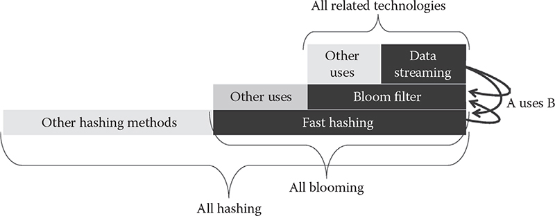
Figure 14.1 The ladder of technologies covered in this chapter.

The two major objectives posed in this chapter are as follows:

Objective 1: Fast hashing. How to calculate hash functions of arbitrary length data using as few CPU cycles as possible.

Objective 2: Efficient lookup. How to find items in structures of arbitrary size and complexity with the highest achievable efficiency.

These objectives do not necessarily complement each other. In fact, they can be conflicting under certain circumstances. For example, faster hash functions may be inferior and cause more key collisions on average. Such collisions have to be resolved by the lookup algorithm, which should be designed to allow multiple records under the same hash key. The alternative of not using collision resolution is a bad design because it directly results in loss of valuable information.

Data streaming as a topic has appeared in the research community relatively recently. The main underlying reason is a fundamental change in how large volumes of data had to be handled. The traditional way to handle large data (Big Data may be a better term)—which is still used in many places today—is to store the data in a database and analyze it later, where the latter is normally referred to as offline [4]. As the Big Data problem—the problem of having to deal with an extremely large volume of data—starts to appear in many areas, storing data in any kind of database has become difficult and in some cases impossible. Specifically, it is pointless to store Big Data if its arrival rate exceeds processing capacity, by the way of logic.

Hence the data streaming problem, which is defined as a process that extracts all the necessary information from an input raw data streamwithout having to store it. The first obvious logical outcome from this statement is that such processing has to happen in real time. In view of this major design feature, the need for both fast hashing and efficient lookup should be obvious.

There is a long list of practical targets for data streaming. Some common targets are

• Calculating a median of all the values in the arrival stream

• Counting all the distinct items

• Detecting the longest increasing or decreasing sequence of values

It should be obvious that the first two targets in the above list would be trivial to achieve without any special algorithm had they come without the conditions. For example, it is easy to calculate the average—simply sum up all the values and divide them by the total number of values. The same goes for the counting of distinct items. This seemingly small detail makes for the majority of complexity in data streaming.

Including the above, the following describes the catch of data streaming:

• There is limited space for storing current state; otherwise, we would revert back to the traditional database-oriented design.

• Data have to be accessed in their natural arrival sequence, which is the obvious side effect of a real-time process—again, a major change from the database-backed processes that can access any record in the database.

• There is an upper limit on per-unit processing cost that, if violated, would break the continuity of a data streaming algorithm (arguably, buffering can help smoothen out temporary spikes in arrival rate).

Note that all the above topics have deep roots in information theory. There is a long list of literature on the topic, of which this author can recommend a recently published book at [2], which discusses modern methods in hashing and blooming (blooming means “using Bloom filters”). There is also a recent book specifically on hashing [3] that provides even more detail on Bloom filters as one of the most popular end uses of hash functions. To the knowledge of this author, there is not yet a book on data streaming given that the topic is relatively new, with early publications dated around 2004.

For the background on the information theory underlying all three main topics in this chapter, the reader is recommended to refer to the above books as well as a long list of literature gradually introduced throughout this chapter.

This chapter itself will try to stick to the minimum of mathematics and will instead focus on the practical methods and algorithms. Practical here partly refers to C/C++ implementations of some of the methods. This chapter has the following structure. Section 14.2 establishes basic terminology. The data streaming problem is introduced in detail in Section 14.3. Section 14.4 talks about simple 32-bit hashing methods. Sections 14.5 and 14.6 discuss practical data streaming and fast hashing, respectively, and Section 14.7 presents a specific practical application for data streaming—extraction of many-to-many communication patterns from packet traffic. The chapter is summarized in Section 14.8.

Note that the C/C++ source code discussed in this chapter is publically available at [43].

14.2 Terminology

As mentioned before, the terms data streams, data streaming, and streaming algorithms all refer to the same class of methods.

Bloom filter or Bloom structure refers to a space in memory that stores the current state of the filter, which normally takes the form of a bit string. However, the Bloom filter itself is not only the data it contains, but also the methods used to create and maintain the state.

Double-linked list (DLL) is also a kind of structure. However, DLLs are arguably exclusively used in C/C++. This is not 100% true—in reality, even this author has been able to use DLLs in other programming languages like PHP or Javascript—but C/C++ programs can benefit the most from DLLs because of the nature of pointers in C/C++ versus that in any other programming language. DLLs refer to a memory structure (struct in C/C++) alternatively to traditional lists—vectors, stacks, etc. In DLLs, each item/element is linked to its neighbors via raw C/C++ pointers, thus forming a chain that can be traversed in either direction. DLLs are revisited later in this chapter and are part of the practical application discussed at the end of the chapter.

The terms word, byte, and digest are specific to hashing. The word is normally a 32-bit (4-byte) integer on 32-bit architectures. A hashing method digests an arbitrary length input at the grain of byte or word and outputs a hash key. Hashing often involves bitwise operations where individual bits of a word are manipulated.

This chapter promised minimum of mathematics. However, some basic notation is necessary. Sets of variables a, b, and c are written as {a, b, c} or {a}_n if the set contains n values of a parameter a. In information theory, the term universe can be expressed as a set.

Sequences of m values of variable b are denoted as <b>_m. Sequences are important for data streaming where sequential arrival of input is one of the environmental conditions. In the case of sequences, m can also be interpreted as window size, given that arrival is normally continuous.

Operators are denoted as functions; that is, the minimum of a set is denoted as min{a, b}.

14.3 The Data Streaming Problem

As mentioned before, data streaming has a relatively small body of literature on the subject. Still, the seminal paper at [14] is a good source for both the background and advanced topics in relation to data streaming. The material at [15] is basically lecture notes published as a 100+-page journal paper and can provide even more insight as well as very good detail on each point raised in this chapter.

This section provides an overview of the subject and presents the theory with its fundamental formulations as well as practical applications and designs. The last subsection presents a summary of current research directions in relation to the core problem.

14.3.1 Related Information Theory and Formulations

We start with the universe of size n. In data streaming we do not have access to the entire universe; instead, we are limited to the current window of size m. The ultimate real-time streaming is when input is read and processed one item at a time, i.e., m =1.

Using the complexity notation, the upper bound for the space (memory, etc.) that is required to maintain the state is

S = O (min {m, n})

If we want to build a robust and sufficiently generic method, it would pay to design it in such a way that it would require roughly the same space for a wide range of n and m, that is,

S = O (log(min {m, n}))

When talking about space efficiency, the closest concept in traditional information theory is channel capacity (see Shannon for the original definition [1]). Let us put function f({a}_n) as the cost (time, CPU cycles, etc.) of operation for each item in the input stream. The cost can be aggregated into f({a}_n) to denote the entire output. It is possible to judge the quality of a given data streaming method by analyzing the latter metric. The analysis can extend into other efficiency metrics like memory size, etc., simply by changing the definition of a per-unit processing cost.

A simple example is in order. Let us discuss the unit cost defined as

f ({a}_n) = f {i : a_i = C}, i … 1, ..., n

The unit cost in this case is the cost of defining—for each item in the arrival stream—if it is equal to a given constant C. Although it sounds primitive, the same exact formulation can be used for a much more complicated unit function.

Here is one example of a slightly higher complexity. This time let us phrase the unit cost as the following condition. Upon receiving item a_i, update a given record f_j ← f_j + C. This time, prior to updating a record, we need to find the record in the current state. Since it is common that i and j have no easily calculable relation between the two, finding the j efficiently can be a challenge.

Note that the above formulations may make it look like data streaming is similar to traditional hashing, where the latter also needs to update its state on every item in the input. This is a gross misrepresentation of what data streaming is all about. Yes, it is true that some portion of the state is potentially updated on each item in the arrival stream. However, in hashing the method always knows which part of the state is to be updated, given that the state itself is often just a single 32-bit word. In data streaming, the state is normally much larger, which means that it takes at least a calculation or an algorithm to find a spot in the state that is to be updated. The best way to describe the relation between data streaming and hashing is to state that data streaming uses hashing as one its primitive operations. Another primitive operation is blooming.

The term sketch is often used in relation to data streaming to describe the entire state, that is, the { f }_m set, at a given point of time. Note that f here denotes the value obtained from the unit function f (), using the same name for convenience.

14.3.2 Practical Applications and Designs

Early proposals related to data streaming were abstract methodologies without any specific application. For example, [15] contains several practical examples referred to as puzzles without any overlaying theme. Regardless, all the examples in early proposals were based on realistic situations. In fact, all data streaming targets known today were established in the very early works. For example, counting frequent items in streams [17] or algorithms working with and optimizing the size of sliding windows [18] are both topics introduced in early proposals.

Data streaming was also fast to catch up with the older area of packet traffic processing. Early years have seen proposals on data streaming methods in Internet traffic and content analysis [14], as well as detection of complex communication patterns in traffic [19, 25]. The paper in [25] specifically is an earlier work by this author and is also this author’s particular interest as far as application of data streaming to packet traffic is concerned. The particular problem of detecting complex communication patterns is revisited several times in this chapter.

Figure 14.2 shows the scenario in which data streaming can be applied to detection of many-to-many communication patterns. The figure is split into upper and lower parts, where the upper partre presents conventional, and the lower the new method based on data streaming. The traditional process collects and stores data for later offline processing. The data streaming process removes the need for storage—at least in the conventional sense, given small storage is still used to maintain the state—and aggregates the patterns in real time. Note that this process also allows for real-time analysis because the data can easily be made available once they are ready. In software, this is normally done via timeouts, where individual records are exported after a given period of inactivity, which naturally indicates that a pattern has ended.

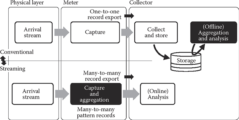
Figure 14.2 A common design for data streaming on top of packet traffic.

Data streaming has been applied to other areas besides traffic. For example, [16] applies the discipline to detection of triangles in large graphs, with obvious practical applications in social networks, among many other areas where graphs can be used to describe underlying topology.

14.3.3 Current Research Topics

Figure 14.3 shows the generic model of a data streaming situation. The parameters are arrival rate, record size, record count, and the index, where the last term is a replacement term for data streaming. Note that only arrival rate is important, because departure rate, by definition, cannot be higher than the arrival rate. On the other hand, arrival rate is important because a data streaming method has to be able to support a given rate of arrival in order to be feasible in practice.

Arrival rate is also the least popular topic in related research. In fact, per-unit processing time is not discussed much in literature, which instead focuses on efficient hashing or blooming methods. Earlier work by this author in [36] shows that per-unit processing cost is important—the study specifically shows that too much processing can have a major impact on throughput.

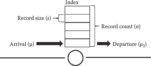
Figure 14.3 Common components shared by all data streaming applications.

The topic of arrival rate is especially important in packet traffic. With constantly increasing transmission rates as well as traffic volume, a higher level of efficiency is demanded of switching equipment. Click router is one such technology [34] that is in active development phase with recent achievements of billion pps processing rates [35]. The same objectives are pursued by OpenVSwitch—a technology in network virtualization. It is interesting that research in this area uses roughly the same terminology as is found in data streaming. For example, [35] is talking about space efficiency of data structures used to support per-packet decision making. Such research often uses Bloom filters to improve search and lookup efficiency. In general, this author predicts with high probability that high-rate packet processing research in the near future will discover the topic of data streaming and will greatly benefit from the discovery.

14.4 Simple 32-Bit Fast Hashing

Hashing is the best option for a store-and-lookup technology. While there are other options like burst trees, hash tables have been repeatedly proven to outperform their competitors [6].

The book at [3] is a good source of the background on hashing. Unfortunately, the book does not cover the topic of fast hashing, which is why it is covered in detail in this chapter. In fact, hashing performance is normally interpreted as statistical quality of a given hash function rather than the time it takes to compute a key.

One of the primary uses for fast hashing in this chapter is lookup. For example, [12] proposes a fast hashing method for lookup of per-flow context, which in turn is necessary to make a decision on whether or not to capture a packet. Note that lookup is not the only possible application of hashing. In fact, message digests and encryption might greatly outweigh lookup if compared in terms of popularity.

The target of this section is to discuss hashing defined as manipulations of individual 32-bit words subject to obtaining quality hash keys. Note that there is a perfect example of such a work in traffic—an IPv4 address. This chapter revisits practical applications in traffic processing and even works with real packet traces like those publicly available at [46] and [47].

14.4.1 Hashing and Blooming Basics

Figure 14.4 presents the basic idea about hashing and blooming in one figure. Although blooming is not covered much in this figure, presenting the two together helps by presenting how the two technologies fit together.

Hashing—the same as applying a hash function on an arbitrary length message—produces an output in the form of a bit string of a given length. The 32-bit hash keys are common—hence the title of this section.

The main point about a hashing method is the quality of a hash key it produces. The subject of quality and its evaluation is covered further in this section.

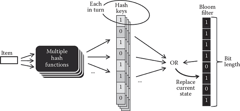
Figure 14.4 Generic model of hashing used in the context of blooming.

Now, here is how the Bloom filter puts hashing to practical use. In the official definition, a Bloom filter can use multiple hash functions for each insert or lookup operations—the number is obviously the same for both operations in the same setting.

Each hash function produces its own bit string. This string is then merged with the current state of the Bloom filter via the bitwise OR operation, the result of which is stored at the new state of the filter. The same is done for each of the multiple hash functions provided there is more than one (not necessarily the case in practice).

It should be obvious that bit lengths of the Bloom filter and each hash key should be the same.

This, in a nutshell, describes the essence of hashing and blooming. The concepts are developed further in this chapter.

14.4.2 Traditional Hashing Methods

Konheim [3] lists all the main classes of hash functions. This subsection is a short overview.

Perfect hashing refers to a method that maps each distinct input to a distinct slot in the output. In other words, perfect hashing is perfect simply because it is free of collisions.

Minimal perfect hashing is a subclass of perfect hashing with the unique feature that the count of distinct items on the output equals that on the input regardless of the range of possible value on the input. This confusing statement can be untangled simply by noting that minimal perfect hashing provides very space efficient outputs. This is why this method is actively researched by methods that require space-efficient states while streaming the data.

Universal hashing is a class of randomized hashing. Note that most methods—including those used in packet traffic, the most famous of which is arguably the CHECKSUM algorithm, also known as the cyclic redundancy check (CRC) family—are deterministic and will always produce the same output for the same input. Randomized hashing is often based on multiplication, which is also known in hashing as “the most time consuming operation” [8]. For this reason alone, fast hashing avoids some of the methods in the universal class.

There are several other classes, like message digests and generally cryptography, both of which have little to do with fast hashing.

The study in [7] is an excellent performance comparison of several popular hash functions and will provide better background on the subject.

14.4.3 Hashing by Bit Manipulation

Bit manipulation is a basic unit of action in hashing. Most existing methods, especially those that are supposed to be fast, are based on bitwise operations. Here is a practical example that shows how the CRC24 method creates its keys (the full implementation of the algorithm can be found in crc24.c at [43]):

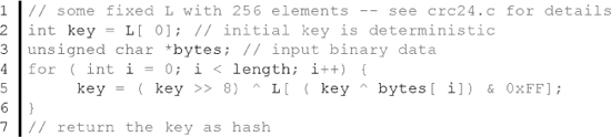
Let us analyze what is happening in this code. First, there is some variable L that contains deterministic values for each of the 256 states it carries. The states are accessed by using the tail of each actual byte from the input stream. The function also makes use of two XOR operations. The initial value of key is set as the first element of L, but then it evolves as it moves through the bytes filtered through predetermined values at various spots in L. All in all, the method looks simple in code, but it is known to provide good quality hash keys. The actual meaning of the word quality is covered later in this section.

As far as bitwise manipulations are concerned, they can be classified into reversible versus irreversible operations. Although keys do not always have to be reversible to be feasible in practice, it is important to know which are which.

The following operations are reversible:

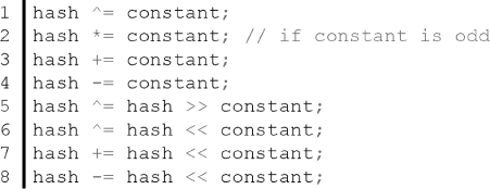
The following operations are nonreversible:

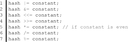
The multiplication operation is a special case not only because it is reversible only if the constant is odd, but also because it incurs more cost than, say, the bitwise shift. It is trivial to understand why bitwise shift to the left is the same as multiplying a number by 2. However, the two operations are very different on most hardware architectures, specifically in the number of CPU cycles an operation incurs or can potentially incur in case the cost is not a fixed number of cycles. Hardware implementation is revisited further in this chapter.

14.4.4 Quality Evaluation of Hash Functions

Quality estimation of a hash function is common knowledge. The following are the main metrics:

Uniform distribution. The output of a hash function should be uniformly distributed. This means that each combination of bits in the output should be equally likely to occur. This metric is easy to test and analyze statistically. Simply collect a set of outputs and plot their distribution to see if it forms a roughly horizontal line.

Avalanche condition. This is a tricky metric that is both the objective of a hash function and the metric that evaluates its quality. The statement is that a change in any one bit on the input should affect every output bit with 50% probability. There is one easy way to understand this metric. If our input changes only in one bit (say, an increment of one), the output should change to a very different bit string from the one before. In fact, the 50% rule says that on average, the XOR difference between the two keys should roughly have 50% of its bits set to 1. Note that this applies to any input bit, meaning that large change in input should cause about the same change in output as a small change in input. Another way to think about this metric is by realizing that this is how the uniform distribution is achieved in the first place.

No partial correlation. There should be no correlation between any parts of input versus output bit strings. Again, this metric is related to both the above metrics but has its own unique underlying statistical mechanisms. Correlation is easy to measure. Simply take time series of partial strings in input versus output and see if the two correlate. You will have to try various combinations—that is, x bits from the head, tail, in the middle, etc.

One-way function. The statement is that it should be computationally infeasible to identify two keys that produce the same hash value or to identify a key that produces a given hashvalue. This metric is highly relevant in cryptography, but is not much useful for fast hashes.

14.4.5 Example Designs for Fast Hashing

There are two fundamental ways to create a fast hashing method:

Create a more efficient method to calculate hash keys while retaining the same level of quality (metrics were discussed above).
Use a simple—and therefore faster—hashing method and resolve quality problems algorithmically.

Arguably, these two methods are the opposite extremes, while the reality is a spectrum between the two. Regardless, the rest of this section will show how to go about writing each of the two algorithms.

The d-left method in [13] is a good example of a fast hashing method that attempts to retain the quality while speeding up calculations. The method uses multiple hash functions for its Bloom filter but proposes an algorithm that avoids using all the functions when calculating each key. In fact, each time the algorithm skips one of k functions, it saves calculation time. The study formulates the method as an optimization problem where the number of overflows is to be minimized. Some level of overflow is inevitable under the method since the space is minimized for faster access. The point therefore is to find a good balance in the trade-off between high number of overflows (basically lost/missed records) and fast hash calculations.

While the above method is scientifically sound, practice often favors simple solutions. Earlier work by this author is one such example [38]. What it does is use simple CRC24 as the only hashing function—thus causing lower quality of keys in terms of collisions, especially given that the keys feature the compression ratio of over five times (141 bits are compressed into 24). This quality problem is dealt with algorithmically using the concept of sideways DLL.

Figure 14.5 shows the basic idea behind sideways DLL. Virtual stem in the figure is the traditional DLL where each item is connected to its neighbor using the traditional to C/C++ variables prev and next. These variables are assigned pointers to neighboring items, thus forming a list-like chain that can be traversed.

Since simple hashing will have higher number of collisions on average, they have to be resolved programmatically. The horizontal chain in Figure 14.5 is one obvious solution. All items in the horizontal chain share the same hash key and are connected into the DLL chain using sidenext and sideprev pointers.

The collisions are resolved as follows. Fast hashing quickly provides a key. The program finds the headmost DLL item for that key. However, there is no guarantee that the headmost element is the correct one—hence the collision. So, the program has to traverse the chain and check whether a given item is the one it is looking for. Granted that such a resolution will also waste CPU cycles, this performance overhead is not fixed for each lookup. In fact, this author’s own practice shows that less than 5% of keys will have sideways chains, while the rest will have only one item in each slot.

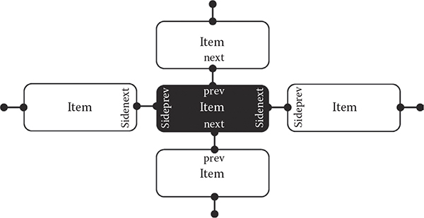
Figure 14.5 Example DLL design that can deal with hash key collisions using the ability to traverse DLL sideways.

The following is the actual C/C++ code for a DLL structure with sideways chains:

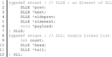
Note that the chain itself is built by DLL element (DLLE) only. Yet, the DLL part is also necessary, especially for traversal. It is also useful to be able to traverse the chain from both the head and the tail. Here is the list of some of the useful properties of DLLs:

• It is easy for two DLLEs to swap positions, which can be done simply by changing assignments in next and prev pointers—the same way any DLLE can be moved to the head or the tail of the DLL.

• Given the easy swapping, it is possible to put a recently used DLLE at the head of the DLL so that it is found first during the next traversal; this way old DLLEs will naturally sink to the bottom (tail) of the DLL. This can also be described as a natural sorting of the DLL by last used timestamp.

• Given the above property, garbage collection is easy—simply pick the oldest DLLEs at the tail of the DLL and dispose of them (or export them, etc.).

DLL is commonplace in packet traffic processing where C/C++ programming is in the overwhelming majority [20]. Earlier research by this author [25] makes extensive use of DLLs. A similar example will be considered as a practical application further in this chapter.

14.5 Practical Data Streaming

This section puts together all the fundamentals presented earlier as part of practical data streaming. The scope of the practice extends from the contents of the input stream to fairly advanced practical data streaming targets.

14.5.1 Distributions in Practice

Research in [41] was the first to argue that traditional distributions, of which beta, exponential, Pareto, etc., are the most common, perform badly as models of natural processes. In fact, this phenomenon was noticed in packet traffic many years before. Yet, research in [41] is the first to present a viable alternative based on the concept of hotspots. The research shows that hotspots are found in many natural systems.

Many statistics collected from real processes support the notion of hotspots. For example, [42] shows that hotspots and flash events exist in data centers that are part of large-scale cloud computing.

Earlier work by this author in [37] developed a model that can synthesize flash events in packet traces. The output of such a synthesis is a packet trace that looks just like a real trace, only with all the timestamps and packet sizes being artificially created by the model.

The model in [37] is based on a stick-breaking (SB) process, which in Figure 14.6 is compared to one of the traditional choices—the beta distribution. The SB process is known to create more realistic power-law distributions—hence its selection as the underlying structure. For realistic traces, not only synthetic sources but also their dynamics are important, which is why a large part of the synthesis is dedicated to creating flash events (left bottom plot of the figure). The modeling logic is simple and is evident from the plot—locations (sources, destinations, content items, etc.) that are already popular can “go viral,” which is where the access count can grow substantially for a limited period of time.

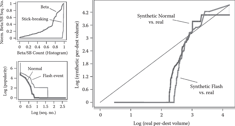
Figure 14.6 The stick-breaking process (left) used to create a synthetic trace versus beta distribution as a common traditional choice, and comparison of the synthetic trace to a real one (right).

The right-side plot in Figure 14.6 shows that even such an elaborate synthesis fails to emulate reality. The plot shows that only the upper 30% of the trace (top flows by volume) closely follows the real distribution, where the resemblance in smaller flow size is almost completely gone. Note that the real packet traces used in comparison come from [47].

Nevertheless, even with the relatively high error margin, synthetic traces are preferred in trace-based simulations specifically because they allow us to test various conditions simply by changing the parameters during synthesis. In this respect, real traces can be considered as the average or representative case, while synthetic traces can be used to test the limits of performance in some methods.

Traces—both real and synthetic—are related to fast hashing via the notion of arrival rate introduced earlier in this chapter. If the method is concerned with per-unit processing cost, the contents of the input stream are of utmost importance. In this respect, packet traffic research provides a fresh new prospective on the subject of fast hashing. While traditionally fast hashing is judged in terms of the quality of its keys, this chapter stresses the importance of the distribution in the input stream.

As far as real packet traces are concerned, CAIDA [48], WAND [46], and WIDE [47] are good public repositories and contain a wide variety of information at each site.

The above synthetic method is not the only available option. There are generators for workloads in many different disciplines, where, for example, RUBIS is a generator of workloads for cloud computing. RUBIS generates synthetic request arrival processes, service times, etc. [49].

14.5.2 Bloom Filters: Store, Lookup, and Efficiency

The study in [9] provides a good theoretical background on the notion of Bloom filters. This section is a brief overview of commonly available information before moving on to the more advanced features actively discussed in research today.

Remember Figure 14.4 from before? Some of this section will discuss the traditional design presented by this figure, but then replace it with a more modern design. From earlier in this chapter we know that blooming is performed by calculating one or more hash keys and updating the value of the filter by OR-ing each hash key with its current state. This is referred to as the insert operation. The lookup operation is done by taking the bitwise AND between a given hash key and current state of the filter. The decision making from this point on can go in one of the following two directions:

• The result of AND is the same as the value of the hash key—this is either true positive or false positive, with no way to tell between the two.

• The result of AND is not the same as the value of the hash key—this is a 100% reliable true negative.

One common way to describe the above lookup behavior of Bloom filters is to describe the filter as a person with memory who can only answer the question “Have you seen this item before?”reliably. This is not to underestimate the utility of the filter, as the answer to this exact question is exactly what is needed in many practical situations.

Let us look at the Bloom filter design from the viewpoint of hashing, especially given that the state of the filter is gradually built by adding more hash keys onto its state.

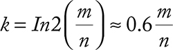
Let us put n as number of items and m the bit length of hash keys, and therefore the filter. We know from before that each bit in the hash key can be set to 1 with 50% probability. Therefore, omitting details, the optimal number of hash function can be calculated as

If each hash function is perfectly independent of all others, then the probability of a bit remaining 0 after n elements is

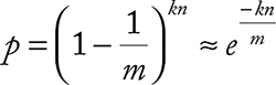
False positive—an important performance metric of a Bloom filter is then

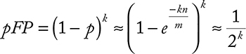
for the optimal k. Note with that increasing k, the probability of false positive is actually supposed to decrease, which is an unintuitive outcomebecause one would expect the filter to get filled up with keys earlier.

Let us analyze the k. For the majority of cases m << n, which means that the optimal number of hash functions is 1. Two functions are feasible only with m > 2.5n. In most realistic cases this is almost never the case because n is normally huge, while m is something practical, like 24 or 32 (bits).

14.5.3 Unconventional Bloom Filter Designs for Data Streams

Based on the above, the obvious problem in Bloom filters is how to improve their flexibility. As a side note, such Bloom filters are normally referred to as dynamic.

The two main changes are (1) extended design of the Bloom filter structure itself, which is not a bit string anymore, and (2) nontrivial manipulation logic dictated by the first change—simply put, one cannot use logical ORs between hashes and Bloom filter states.

Figure 14.7 shows the generic model that applies to most of the proposals of dynamic Bloom filters. The simple idea is to replace a simple bit string with a richer data structure (the change in the Bloom filter in the figure). Each bit in the filter now simply is a pointer to a structure that supports dynamic operations.

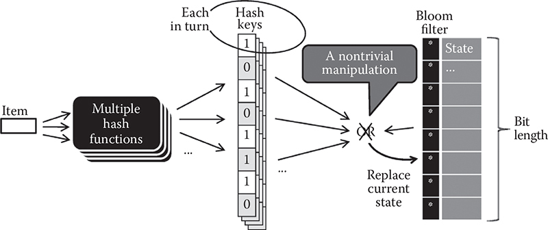
Figure 14.7 A generic model representing Bloom filters with dynamic functionality.

The other change that ensues is that the OR operation is no longer applicable. Instead, a nontrivial manipulation has to be performed on each bit of the value that was supposed to be OR-ed in the traditional design. Naturally, this incurs a considerable overhead on performance.

The following classes of dynamic Bloom filters are found in literature.

Stop additions filter. This filter will stop accepting new keys beyond a given point. Obviously this is done in order to keep false positive beyond a given target value.

Deletion filter. This filter is tricky to build, but if accomplished, it can revert to a given previous state by forgetting the change introduced by a given key.

Counting filters. This filter can count on both individual bits of potential occurrences of entire values and combinations of bits. This particular class of filters obviously can find practical applications in data streaming. In fact, the example of the d-left hashing method discussed earlier in this chapter uses a kind of counting Bloom filter [13]. Another example can be found in [12], where it is used roughly for the same purpose.

There are other kinds of unconventional designs. The study in [10] declares that it can do with fewer hash functions while providing the same blooming performance. Bloom filters specific to perfect hashing are proposed in [11].

14.5.4 Practical Data Streaming Targets

This subsection considers several practical data streaming targets.

Example 14.1: A Simple Sampling Problem

We need a median of the stream. The problem is to find a uniform sample s from a stream of unknown length and unknown content in advance. Again, by definition, even having seen all the input, we cannot use it because there is not enough storage for its entire volume.

Algorithm:Set originally s = x₁. On seeing the tth element, the probability of s ← x_t is 1/t.

Analysis: The probability that s = x_i at some time t ≥ i is

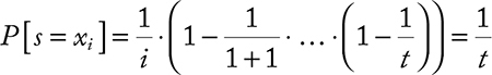
To get k samples, we use O(k log n) bits of space.

Example 14.2: The Sliding Window Problem

Maintain a uniform sample from the last w items algorithm:

• For each x_i pick a random value v_k ∈ (0, 1).

• In a window (x_{_j–w} + 1, …, x_j) return value x_i with smallest the x_i.

• To do this, maintain a set of all elements in a sliding window whose v value is minimal among subsequent values.

Analysis: The probability that the jth oldest element is in S is 1/j, so the expected number of items in S is

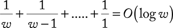
Therefore, the algorithm only uses O(log w log n) bits of memory.

Example 14.3: The Sketch Problem

Apply a linear projection “on the fly” that takes high-dimensional data to a smaller dimensional space. Post-process the lower-dimensional image to estimate the quantities of interest.

Input: Stream from two sources:

(x₁,x₂, ..., x_m,) ∈ (A [n] ∪) B [n])^m

The objective is to estimate the difference between distributions of A values and B values, so

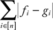
where

fi =|{k : x_k =i}| and g_i = |{k : x_k =i}|

Example 14.4: Count-Min Sketch

For example, we might detect heavy hitters f_i ≥ m, or range sum estimate:

when i, j are not known in advance. For k-quantiles, find values q ₀ , …, q _k such that

Algorithm: Maintain a list of counters c_i,_j for i ∈ [d] and j ∈ [w]. Construct d random hash functions h₁, h₂, …, h_d: [n] → [d]. Update counters, when the encounter value v increment is c_i,h_i (_v)for i ∈ [d]. To get an estimate of f_k return

Analysis: For d = O(log(1/δ)) and w = O(1/ε²),

Example 14.5: The Counting Problem

Count distinct elements in stream.

Input: Stream (x₁, x₂, …, x_m) ∈ [n]^m. The objective is to estimate the number of distinct values in the stream up to a multiplicative factor 1 + ε with high probability.

Algorithm: Apply random function h: [n] ∈ [0, 1] to each element. Compute a—the tth smallest value of the hash seen where t =21/ε². Return r^* = t/a as the estimate of r—the number of distinct items.

Analysis: Algorithm uses O(e^–2 log n) bits of space. Estimate has good accuracy with reasonable probability:

P[| r * - r | ≤∈r] ≤ r ] ≤ 9/10

The proof involves the concept of Chebyshev analysis and is pretty complicated, but it is out there if you do a quick search in the literature provided above.

14.5.5 Higher-Complexity Data Streaming Targets

Besides the relatively simple (you can call them traditional) data streaming targets, there are several interesting practical targets that need a higher level of algorithmic complexity. This subsection lists only the problems and leaves the search for solutions to the reader. In fact, some solutions are the subject of active discussion in the research community today. Pointers to such research are provided.

Example 14.6: Finding Heavy Hitters (beyond the Min-Count Sketch)

Find k most frequently accessed items in a list. One algorithm is proposed in [17]. Generally, more sound algorithms for sliding windows can be found in [18].

Example 14.7: Triangle Detection

Detect triangles defined as A talks to B, B talks to C, and C talks to A (other variants are possible as well) in the input stream. An algorithm is proposed in [16].

Example 14.8: Superspreaders

Detect items that access or are accessed by exceedingly many other items. Related research can be found in [19].

Example 14.9: Many-to-Many Patterns

This is a more generic case of heavy hitters and superspreaders, but in this definition the patterns are not known in advance. Earlier work by this author [25] is one method. However, the subject is popular with several methods, such as M2M broadcasting [26] and various M2M memory structures [27, 31], and data representations (like graph in [28]) are proposed—all outside of the concept of data streaming. The topic is of high intrinsic value because it has direct relevance to group communications where one-to-many and many-to-many are the two popular types of group communications [29, 30, 32, 33].

A practical example later in this chapter will be based on a many-to-many pattern capture.

14.6 Practical Fast Hashing and Blooming

This section expands further into the practical issues in relation with fast hashing and blooming.

14.6.1 Arbitrary Bit Length Hashing

Obvious choices when discussing long hashes are the MD5 and SHA-family of methods.

It is interesting that bit length is about the only difference of such methods from simpler 32-bit hash keys. The state is still created and updated using bitwise operations, with the only exception that the state now extends over several words and updates are made by rotation.

Both groups of methods are created with hardware implementation in mind where it is possible to update the entire bit length or even digest the entire message in one CPU cycle.

The methods, however, are useless for data streaming in general, mostly due to the long bit length. With CRC24, it is possible to procure a memory space with 2²⁴ memory slots (where each slot is a 4-byte C/C++ pointer). But there is no feasible solution for a memoryregion addressable using an MD5 key as an index.

However, given the uniform distribution condition, it is possible to use only several bits from any region of the hash key. However, given that MD5 or SHA- methods take much longer to compute than the standard CRC24 or even a simpler bitwise manipulation, such a use would defeat the purpose of fast hashing.

14.6.2 Arbitrary Length Bloom Filters

Again, using longer Bloom filters has dubious practical value. Based on the simple statistics presented above, increasing the bit length of the filter only makes sense when it helps increase the number of hash functions. However, the equation showed that increase in bit length is reduced by 40%. Even before that, m is part of the ratio m/n, which makes it nearly impossible to have any practical impact n when n is large. In practice, n is always large.

In view of this argument, it appears that the dynamic filters presented earlier in this paper present a better alternative to using longer bit strings in traditional Bloom filters.

14.6.3 Hardware Implementation

Hashing is often considered in tandem with hardware implementation. The related term is hardware offload—where a given operation is offloaded to hardware. It is common to reduce multi-hundred-cycle operations to single CPU cycles. This subsection presents several such examples.

One common example is to offload CHECKSUM calculations to hardware. For example, the COMBO6 card [20] has done that and has shown that it has major impact on performance.

Note that the most popular hashing methods today—the MD5 and SHA-2 methods—are created with hardware implementation in mind. MD5 is built for 32-bit architectures and has its implementation code in RFC1321 [22], fully publicly open. The SHA-* family of hashing methods are also built for hardware implementation but are still being improved today [24]. One shared feature between these methods is that they avoid multiplication, resorting to simple bitwise manipulations instead.

Two other main threads in hardware offloading are

• GPU-based hardware implementation, specifically using the industry default CUDA programming language [21]

• Memory access optimization where the method itself tries to make as few accesses to memory as possible [23]—although not particularly a hardware technology, such methods are often intimately coupled with specific hardware, like special kind of RAM, etc.

14.7 Practical Example: High-Speed Packet Traffic Processor

This section dedicates its full attention to an example data streaming method from the area of packet traffic processing.

14.7.1 Example Data Streaming Target

Let us assume that there is a service provided by a service provider. The realm of the service contains many users. A many-to-many (M2M) pattern is formed by a subset of these users that communicate among each other. Favoring specificity over generalization, M2M parties can be classified into M2M sources and M2M destinations. While this specificity may not be extended to M2M problems in other disciplines, it makes perfect sense in traffic analysis because flows are directional. Besides, the generality can be easily restored if it is assumed that sources can be destinations, and vice versa. In fact, in many communication patterns today, this is actually the case, which means that two flows in opposite directions can be found between two parties.

Traffic capture and aggregation happens at the service provider (SP), which is the location of convenience because all the traffic that flows through the SP already can be captured without any change in communication procedures.

The problem is then defined as the need to develop a method and software design capable of online capture and aggregation of such M2M patterns.

Note that this formulation is one level up from the superspreaders in [19]. While the latter simply identifies singular IP addresses that are defined as superspreaders, this problem needs to capture the communication pattern itself.

14.7.2 Design for Hashing and Data Structures

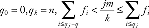
Figure 14.8 shows the rough design of the system. Hash keys of x bits long are used as addressed in the index. Collision avoidance is implemented using sideways DLL, as was described earlier in this chapter (this particular detail is not shown in the figure). Each slot in the index points to an entry that in turn can contain multiple subentries. In this context, entry is the entire multiparty communication pattern, while subentry is its unit component that describes a single communication link between two members of a communication group.

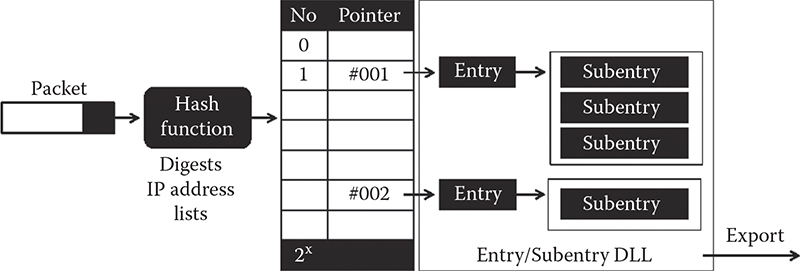
Figure 14.8 Overall design of an index for capturing many-to-many group communication.

Since each pattern can have multiple parties, each with its own IP address, multiple slots in the hash table can point to the same entry. This is not a problem in C/C++, where the same pointer can be stored in multiple places in memory.

Figure 14.9 finally reveals the entire data structure. The source code can be found in m2meter.c at [43]. The design is shown in the manner traditional to such systems where the actual bit lengths of all parts are marked. The unit (the width of each part) is 32 bits. Note that the word can be split into smaller bit strings, as they can be handled by bitwise operations in C/C++ with relative ease.

The following parts of the figure are relatively unimportant. Timestamp log is not crucial for this particular operation, as well as from the viewpoint of data streaming. However, if necessary, timestamps—where each word is a bitwise merger of sublist ID and the timestamp of the last activity of that particular sublist—can be stored in sequence after the source header in entry. Also, the design of the conventional meter—that is used in traditional flow-based packet capture—is shown for reference.

Below the level of entry there are sublists where each sublist is a DLL containing subentries. The actual hierarchy is as follows.

Figure 14.9 The actual data structure compared to the traditional one-to-one flows.

Each entry has a DLL of sublists, and each sublist has a DLL of subentries. Although slightly confusing, the intermediate step of thesublist is necessary as an efficiency mechanism where the mechanism itself is explained further on.

Bloom filters are an important part of operation. First, there is global Bloom, which is used to find out right away if a given subentry has been created earlier in this entry. In a sense, this is a form of collision control at the time when deciding whether or not to create a new subentry. Sublists also have each their own sublist Bloom, which is used for the same purpose, only within the bounds of each sublist. This is in fact the sole purpose of each sublist—to split all subentries into smaller groups to improve lookup performance.

Let us consider how this structure performs in practice. The entry itself is accessed directly via a hash key; there is zero ambiguity in this operation. Each access needs to either create new or update a subentry inside the entry. The following sequence of actions is performed:

• First, global Bloom is queried, resulting in either true negative, true positive, or false positive, with no way to tell the difference between the latter two outcomes. True negative is the best outcome because it tells us that we can go ahead and create a new subentry, as we are certain that no such subentry has been created in this entry before. In case of either of the two positives, we have to verify the outcome by traversing the DLL of sublists. To facilitate this traversal, the entry has a pointer to the last used sublist. Regardless of the outcome, global Bloom has to be updated using the current subentry hash key.

• We are at this step because global Bloom produced a positive outcome. Traversing the list of sublists, each sublist Bloom is queried using the same subentry hash key. Again, either a true negative or positive outcome can be produced. If true negative, we move on to the next sublist. If we run out ofsublists, it means that a subentry is not found, which in turnmeans that we need to create a new subentry. In the case of a positive outcome, we need to traverse the subentry DLL of the respective sublist, to either find the subentry we are looking for or verify that the positive outcome is a false positive.

Note that with all the algorithmic complexity, the purpose is simply to improve lookup time as often as possible. This means that the system needs to achieve a relatively higher ratio of true negatives to positive outcomes on all the Bloom filters.

The data structure in Figure 14.9 can be further improved. For example, one obvious problem is with the global Bloom, which gets filled up too fast. Potentially, it can be replaced with a dynamic filter, as was described earlier in this chapter. However, keep in mind that there are potentially 2²⁴ such Bloom filters in the entire structure, which means that if dynamic filters are used, they have to be extremely efficient in terms of the space they occupy. The use of dynamic filters would also potentially remove the need for sublists, which would simplify the design of each entry.

14.8 Summary

This chapter discussed the topic of fast hashing and efficient blooming in the context of data streaming. Higher efficiency in both the former operations are demanded by the operational realities of data streaming, which are forced to run under very strict per-unit processing deadlines.

Having reviewed all the existing methods in both hashing and blooming, the following two extreme designs were presented in detail. At one extreme was a data streaming method that invests heavily into developing a faster hashing method without losing the quality of its hash keys. At the other extreme was a method that selects the lightest possible hash function at the cost of reduced quality, but resolves key collisions programmatically. The designs are presented without any judgment as to which method is better. However, in reality, it is likely that real methods will form a spectrum in between the two extremes.

Note that the same can be said about Bloom filters as well. The two extremes in this case are traditional versus dynamic Bloom filters, where dynamic ones require much heavier calculation overheads to maintain and use. While analyzing the practical application in the last section, it was stated that dynamic Bloom filters might help to improve lookup performance, provided the overhead would stay below the one caused by the programmatic method presented in the example.

There are several topics that are immediately adjacent to the main topic in the chapter. For example, the closest other topic is that of multicore architectures. Good shared memory designs for C/C++ can be found in [5]. A lock-free shared memory design developed by this author can be found at [44]. These subjects are related because data streaming on multicore needs to be extremely efficient, beyond the level that can be offered with traditional parallel processing designs based on memory locking or message passing. Note that the subject of multicore is already a hot topic [40] in traffic. The title of such research can be hashing for multicore load balancing.

Alternative methods for traffic processing other than flows can also benefit from fast hashing and efficient blooming. For example, earlier work by this author converted traffic to graphics for visual analysis [38]. Also, as was mentioned before, smart traffic sampling can be directly formulated as a data streaming problem [39]. Such a formulation is yet to be adopted by the research community. The key term is context-based sampling in traffic research, but would be rephrased as packet streaming when viewed as a data streaming problem.

Since hashing is a large part of indexing and even broader, search, fast hashing can help new areas where indexing is starting to find its application. For example, Fullproof at [50] is a Lucene indexing engine rewritten from scratch to work in restrictive local storage in browsers (running as a web application). Earlier work by this author proposed a browser-based indexer for cloud storage called Stringex [45], in which the key feature is that read and write access has an upper restriction on throughput. This restriction is very similar to that of CPU operations in fast hashing, which is where the parallel can be drawn.

Broadly speaking, data streaming is yet to be recognized as an important discipline. Once it is recognized as such, however, it will open all the research venues related to fast hashing and dynamic blooming listed in this chapter.

References

1. C. Shannon. A Mathematical Theory of Communication. Bell System Technical Journal, 27, 379–423, 1948.

2. D. MacKay. Information Theory, Inference, and Learning Algorithms. Cambridge: Cambridge University Press, 2003.

3. A. Konheim. Hashing in Computer Science: Fifty Years of Slicing and Dicing. Hoboken, NJ: Wiley, 2010.

4. R. Kimball, M. Ross, W. Thornthwaite, J. Mundy, and B. Becker. The Data Warehouse Lifecycle Toolkit. New York: John Wiley & Sons, 2008.

5. K. Michael. The Linux Programming Interface. San Francisco: No Starch Press, 2010.

6. S. Heinz, J. Zobel, and H. Williams. Burst Tries: A Fast, Efficient Data Structure for String Keys. ACM Transactions on Information Systems (TOIS), 20(2), 192–223, 2002.

7. M. Ramakrishna and J. Zobel. Performance in Practice of String Hashing Functions. In 5th International Conference on Database Systems for Advanced Applications, April 1997.

8. D. Lemire and O. Kaser. Strongly Universal String Hashing Is Fast. Cornell University Technical Report arXiv:1202.4961. 2013.

9. F. Putze, P. Sanders, and J. Singler. Cache-, Hash- and Space-Efficient Bloom Filters. Journal of Experimental Algorithmics (JEA), 14, 4, 2009.

10. A. Kirsch and M. Mitzenmacher. Less Hashing, Same Performance: Building a Better Bloom Filter. Wiley Interscience Journal on Random Structures and Algorithms, 33(2), 187–218, 2007.

11. G. Antichi, D. Ficara, S. Giordano, G. Procissi, and F. Vitucci. Blooming Trees for Minimal Perfect Hashing. In IEEE Global Telecommunications Conference (GLOBECOM), December 2008, pp. 1–5.

12. H. Song, S. Dharmapurikar, J. Turner, and J. Lockwood. Fast Hash Table Lookup Using Extended Bloom Filter: An Aid to Network Processing. Presented at SIGCOMM, 2005.

13. F. Bonomi, M. Mitzenmacher, R. Panigrahi, S. Singh, and G. Vargrese. An Improved Construction for Counting Bloom Filters. In 14th Conference on Annual European Symposium (ESA), 2006, vol. 14, pp. 684–695.

14. M. Sung, A. Kumar, L. Li, J. Wang, and J. Xu. Scalable and Efficient Data Streaming Algorithms for Detecting Common Content in Internet Traffic. Presented at ICDE Workshop, 2006.

15. S. Muthukrishnan. Data Streams: Algorithms and Applications. Foundations and Trends in Theoretical Computer Science, 1(2), 117–236, 2005.

16. Z. Bar-Yossef, R. Kumar, and D. Sivakumar. Reductions in Streaming Algorithms, with an Application to Counting Triangles in Graphs. Presented at 13th ACM-SIAM Symposium on Discrete Algorithms (SODA), January 2002.

17. M. Charikar, K. Chen, and M. Farach-Colton. Finding Frequent Items in Data Streams. Presented at 29th International Colloquium on Automata, Languages, and Programming, 2002.

18. M. Datar, A. Gionis, P. Indyk, and R. Motwani. Maintaining Stream Statistics over Sliding Windows. SIAM Journal on Computing, 31(6), 1794–1813, 2002.

19. S. Venkataraman, D. Song, P. Gibbons, and A. Blum. New Streaming Algorithms for Fast Detection of Superspreaders. Presented at Distributed System Security Symposium (NDSS), 2005.

20. M. Zadnik, T. Pecenka, and J. Korenek. NetFlow Probe Intended for High-Speed Networks. In International Conference on Field Programmable Logic and Applications, 2005, pp. 695–698.

21. S. Manavski. CUDA Compatible GPU as an Efficient Hardware Accelerator for AES Cryptography. In IEEE International Conference on Signal Processing and Communication, 2007, pp. 65–68.

22. The MD5 Message-Digest Algorithm. RFC1321. 1992.

23. G. Antichi, A. Pietro, D. Ficara, S. Giordano, G. Procissi, and F. Vitucci. A Heuristic and Hybrid Hash-Based Approach to Fast Lookup. In International Conference on High Performance Switching and Routing (HPSR), June 2009, pp. 1–6.

24. R. Chaves, G. Kuzmanov, L. Sousa, and S. Vassiliadis. Improving SHA-2 Hardware Implementations. In Cryptographic Hardware and Embedded Systems (CHES), Springer LNCS vol. 4249. Berlin: Springer, 2006, pp. 298–310.

25. M. Zhanikeev. A Holistic Community-Based Architecture for Measuring End-to-End QoS at Data Centres. Inderscience International Journal of Computational Science and Engineering (IJCSE), 2013.

26. C. Bhavanasi and S. Iyer. M2MC: Middleware for Many to Many Communication over Broadcast Networks. In 1st International Conference on Communication Systems Software and Middleware, 2006, pp. 323–332.

27. D. Digby. A Search Memory for Many-to-Many Comparisons. IEEE Transactions on Computers, C22(8), 768–772, 1973.

28. Y. Keselman, A. Shokoufandeh, M. Demirci, and S. Dickinson. Many-to-Many Graph Matching via Metric Embedding. In IEEE Conference on Computer Vision and Pattern Recognition (CVPR), 2003, pp. 850–857.

29. D. Lorenz, A. Orda, and D. Raz. Optimal Partition of QoS Requirements for Many-to-Many Connections. In International Conference on Computers and Communications (ICC), 2003, pp. 1670–1680.

30. V. Dvorak, J. Jaros, and M. Ohlidal. Optimum Topology-Aware Scheduling of Many-to-Many Collective Communications, In 6th International Conference on Networking (ICN), 2007, p. 61.

31. M. Hattori and M. Hagiwara. Knowledge Processing System Using Multidirectional Associative Memory. In IEEE International Conference on Neural Networks, 1995, vol. 3, pp. 1304–1309.

32. A. Silberstein and J. Yang. Many-to-Many Aggregation for Sensor Networks. In 23rd International Conference on Data Engineering, 2007, pp. 986–995.

33. M. Saleh and A. Kamal. Approximation Algorithms for Many-to-Many Traffic Grooming in WDM Mesh Networks. In INFOCOM, 2010, pp. 579–587.

34. E. Kohler, R. Morris, B. Chen, J. Jannotti, and M. Kaashoek. The Click Modular Router. ACM Transactions on Computer Systems (TOCS), 18(3), 263–297, 2000.

35. M. Zec, L. Rizzo, and M. Mikuc. DXR: Towards a Billion Routing Lookups per Second in Software. ACM SIGCOMM Computer Communication Review, 42(5), 30–36, 2012.

36. M. Zhanikeev. Experiments with Practical On-Demand Multi-Core Packet Capture. Presented at 15th Asia-Pacific Network Operations and Management Symposium (APNOMS), 2013.

37. M. Zhanikeev and Y. Tanaka. Popularity-Based Modeling of Flash Events in Synthetic Packet Traces. IEICE Technical Report on Communication Quality, 112(288), 1–6, 2012.

38. M. Zhanikeev and Y. Tanaka. A Graphical Method for Detection of Flash Crowds in Traffic. Springer Telecommunication Systems Journal, 63(4), 2013.

39. J. Zhang, X. Niu, and J. Wu. A Space-Efficient Fair Packet Sampling Algorithm. In Asia-Pacific Network Operation and Management Symposium (APNOMS), Springer LNCS5297, September 2008, pp. 246–255.

40. M. Aldinucci, M. Torquati, and M. Meneghin. FastFlow: Efficient Parallel Streaming Applications on Multi-Core. Technical Report TR-09-12. Universita di Pisa, September 2009.

41. P. Bodík, A. Fox, M. Franklin, M. Jordan, and D. Patterson. Characterizing, Modeling, and Generating Workload Spikes for Stateful Services. In 1st ACM Symposium on Cloud Computing (SoCC), 2010, pp. 241–252.

42. T. Benson, A. Akella, and D. Maltz. Network Traffic Characteristics of Data Centers in the Wild. In Internet Measurement Conference (IMC), November 2010, pp. 202–208.

43. Source code for this chapter. Available at https://github.com/maratishe/fasthash4datastreams.

44. MCoreMemory project page. Available at https://github.com/maratishe/mcorememory.

45. Stringex Project Repository. Available at https://github.com/maratishe/stringex.

46. WAND Network Traffic Archive. Available at http://www.wand.net.nz/wits/waikato/5/.

47. MAWI Working Group Traffic Archive. Available at http://mawi.wide.ad.jp/mawi.

48. CAIDA homepage. Available at http://www.caida.org.

49. Rubis homepage. Available at http://rubis.ow2.org/.

50. Fullproof: Browser Side Indexing. Available at https://github.com/reyesr/fullproof.

..................Content has been hidden....................

You can't read the all page of ebook, please click here login for view all page.

Table of Contents for Chapter 14: Methods and Algorithms for Fast Hashing in Data Streaming

Create new playlist

Sign In

Sign Up

14METHODS AND ALGORITHMS FOR FAST HASHING IN DATA STREAMING

MARAT ZHANIKEEV

Keywords

14.1 Introduction and Practical Situations