The previous chapter was about unpivoting, which is the process of turning columns into rows. The opposite operation is called pivoting, which – surprise, surprise – is turning rows into columns.
The idea is that you have a resultset with some dimensional values in one or more columns and some facts/measure values in one or more other columns. You’d like the output grouped by some other columns, so you only have one aggregated row for those values, and then the values from your measures should be placed in a set of columns, one for each value of your dimension (or combination of values if you have multiple dimensions).
One thing to remember here is that in SQL, the engine needs at parse time to be able to determine names and datatypes of each column. That means that you have to hardcode the dimension values and what column names they should be turned into.
If you wish to have dynamic pivoting, where there automatically will be columns for every dimension value in the data, you need to build it with dynamic SQL similarly to what I showed at the end of the previous chapter. That way there will be a parsing every time you run it, and the column names can then be known at that time. Alternatively the pivot clause supports returning XML instead of columns, which allows you dynamic pivoting without dynamic SQL – which can be an option if an XML output is acceptable. Either way of dynamic pivoting will not be covered in this book.
In Oracle version 18c or newer, there is a third dynamic pivoting method using polymorphic table functions. I won’t be covering PTFs in this book, but Chris Saxon of the Oracle AskTom team has an example of a PTF for dynamic pivoting on Live SQL: https://livesql.oracle.com/apex/livesql/file/content_HPN95108FSSZD87PXX7MG3LW3.html.
Tables for pivoting

Purchases table and associated dimension tables
View joining purchases table with the dimensions
Yearly purchased quantities by brewery and product group
Now I’d like to have a column for quantity purchased each of the three years instead of a row for each year – this is what pivoting is all about.
Pivoting single measure and dimension
Pivoting the year rows into columns
Lines 3–12 simply are the select from Listing 8-2, wrapped in an inline view.
The pivot keyword in line 13 tells Oracle I want to pivot the data.
Then I define my measures – in this case only one, the quantity – in line 14. I must use an aggregate function here – it can be any aggregate, the one that makes sense in this case is sum.
After the keyword for in line 15, I define the dimensions I want – here only the year.
Last, the in clause in lines 16–19 maps in which columns the aggregated measure should be placed for which values of the dimension – columns that do not exist in the table, but will be created in the output.
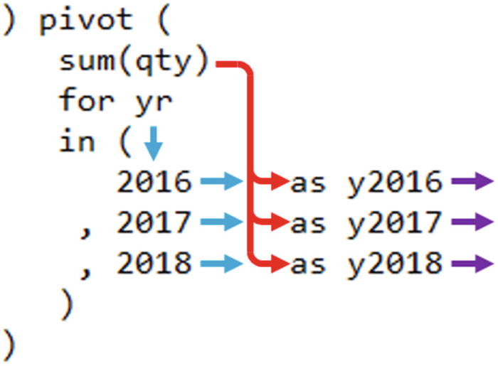
The flows of the pivot clause
Notice that the yr and qty columns from the inline view are no longer in the output, but brewery_name and group_name are. What happens is that those columns I am referencing in the measures and dimensions in the pivot clause are used for the pivoting. The columns that are left over, they are used for an implicit group by.
Since in my inline view I have already grouped the data by brewery, product group, and year, this means that the sum(qty) in line 14 actually always will “aggregate” just a single row of data into each of the year columns, so that aggregation is not really necessary. But I cannot skip it – the pivot clause demands an aggregate function.
Utilizing the implicit group by
Listing 8-4 gives exactly the same output as Listing 8-3; it is just a little bit more efficient from not doing a superfluous grouping operation.
You might think that I could then skip the inline view completely? Well, sometimes it is possible, but not in this case, first because I need to extract the year from the purchased date column and second because the pivot performs an implicit group by on the remaining columns after some of the columns have been used for measures and dimensions.
If I had the yr column in the view and could pivot directly on the purchases_with_dims view, the grouping would be performed on all the columns of the view except qty and yr – it would give me the wrong result. The inline view lets me keep only the columns I need – those to be used in the pivoting and those to be used for the implicit group by.
To make it a little more clear what’s happening behind the scenes with the pivot clause, let me show you pivoting performed manually without pivot.
Do-it-yourself manual pivoting
Manual pivoting without using pivot clause
I do a group by brewery and product group in lines 20–22. And then I have three case structures for each of the three columns I want, so that all rows in the view from the year 2016 will have the qty value summed in column y2016, all rows from 2017 will be summed in y2017, and 2018 in y2018. The output is exactly the same as Listing 8-4 and Listing 8-3.
This structure is built for me automatically when I use the pivot clause. In Listing 8-4, I defined I wanted to use aggregate function sum on the value from column qty, but such that qty for rows in year 2016 goes to a column I want to be named y2016, and so on. I am not defining what to use for the implicit group by – this will be whatever columns are left over, so therefore I am using the inline view to limit the columns that go to the pivot clause rather than use all columns of the view.
Knowing this is the way pivot works will help, when I now show you pivoting with multiple measures by also using the column cost from the table purchases and the view purchases_with_dims, instead of just qty.
Multiple measures
Getting an ORA-00918 error with multiple measures
Why do I get an error saying column ambiguously defined? I haven’t written the same column alias twice? Well, not directly, but indirectly I have.
What happens is that I have defined two measures with no column aliases. Then I have defined the three year values in the yr dimension and column aliases for them. There will be created a column for every combination, so 2 x 3 = 6 columns. Those six columns will be named <dimension alias>_<measure alias>, but if there are no measure aliases, then they will just be named <dimension alias>, as you saw in Listings 8-3 and 8-4. There it was okay, but here it means there will be two columns named y2016, two columns y2017, and two columns y2018. Thus the ORA-00918 error.
The solution is to also give the measures column aliases, so, for example, I can do as shown in Figure 8-3, where I alias the measures simply q and c, while the dimension values are aliased with two digits of the year (since those aliases do not start with a letter, they need to be quoted).
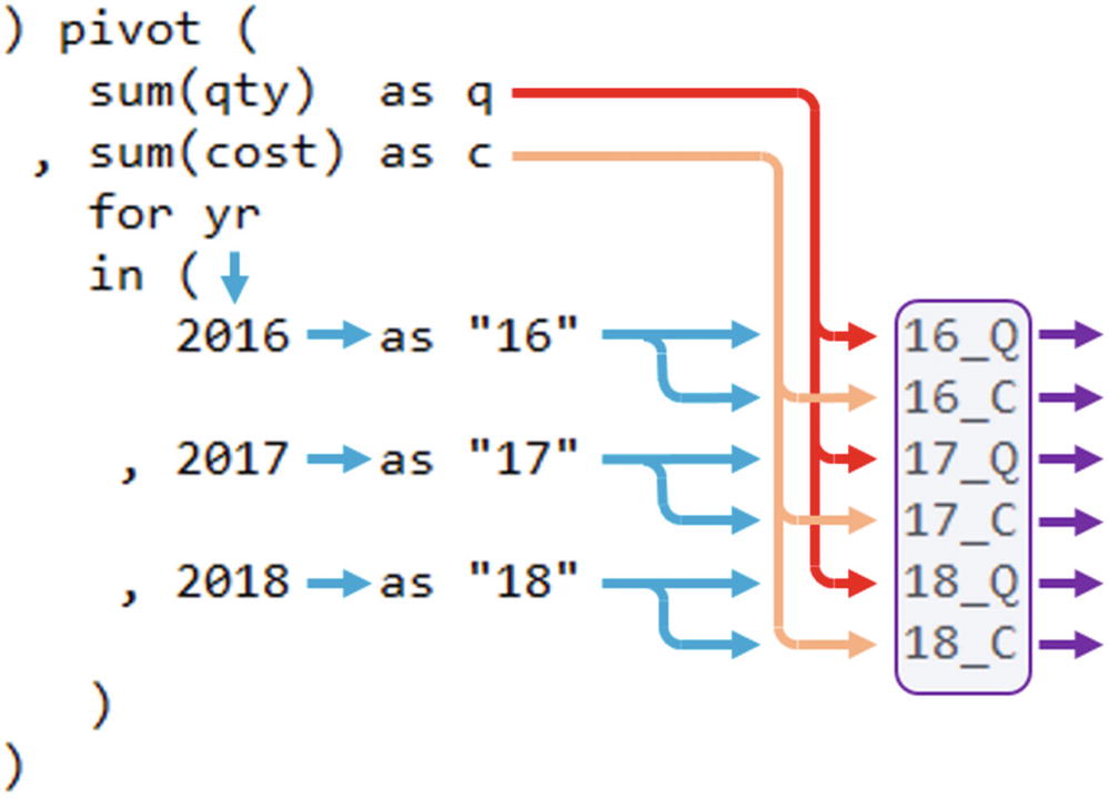
Schematic flow when you have multiple measures
(Normally I’d probably pick a little more descriptive column aliases, but using so short aliases makes the lines fit in a book.)
So I’ve now demonstrated getting pivoted columns as combinations of multiple measures and values of a single dimension. Next up is adding multiple dimensions too.
Multiple dimensions as well
So far I’ve pivoted only with the year as a dimension, leaving brewery and product group as the columns that are used for implicit group by. Now I’m going to also pivot the product group as a second dimension, leaving only the brewery to be grouped upon.
Combining two dimensions and two measures
You’ll notice that the content of the inline view in lines 3–12 is in principle the same as before; I’ve simply added a where clause to reduce the dataset I’m pivoting.
The measures q and c in lines 14–15 are also unchanged, just as they were when I only used a single dimension.
Line 16 is different, since here I am no longer just specifying a single column to be my dimension. I am specifying an expression list of two columns instead – group_name and yr.
And since I use an expression list of two columns in my for clause, I also need to use corresponding expression lists of values in the in clause mappings in lines 18–21. Each value expression list (combinations of dimension values) I give a column alias – in this case a very short alias to keep my lines short enough for print; in real life more meaningful aliases should be used.

Flows with multiple dimensions just have expression lists instead of single expressions
The blanks are because the Good Beer Trading Co does not buy any IPA from Balthazar Brauerei nor any Wheat beers from Brewing Barbarian.
Knowing how the pivoting works as an implicit group by as I showed earlier about do-it-yourself manual pivoting, you can also see that in principle, I did not need to reduce the dataset with the where clause in lines 10–12. I could simply remove those three lines, and my output would be exactly the same. (Since I do have all three breweries in my output already, if I had had breweries with no purchases at all within the years and product groups I’m after, then there’d be output differences in the form of empty rows.)
However, it would not be a good idea to do so, since the data from the other years and other product groups still would be processed; the implicit case structures would just mean no data from those other years and product groups would be added to the aggregate sums. It would be a waste of CPU cycles and I/O.
Lessons learned
Pivoting with the three elements of the pivot clause, measures, dimensions, and mappings
Naming the pivoted columns with measure and dimension aliases, where combinations with multiple measures are automatically joined with underscores
Manual pivoting with group by and aggregation on case structures to aid understanding of how pivot works
Using expression lists for values from multiple dimensions when pivoting
Pivoting is a very useful tool in your toolbox for a variety of things, quite often simply because users get a much better overview of their data if they do not need to read a lot of rows like the output of Listing 8-2, but can have fewer rows with more columns like the various pivoted outputs in the chapter.