One of the most useful features of analytic functions is the flexibility of the window clause, enabling aggregation of particular subsets of the data within a specific order. A classic subset that can be used for many purposes is the set of data from the beginning until the current row – if, for example, the sum aggregate function is used on that subset, you get an accumulated sum or rolling sum or running total (many names for the same thing).
The use cases are plenty; many financial reports need running totals. But a different practical use case that has been extremely helpful in my work involves a slight variation of the running total, where I use the sum of all the previous rows to keep selecting rows until I have selected just sufficiently large subset to cover the sum I need – in this case until I have picked enough goods in the warehouse to cover the order by a customer.
The complete case in this chapter will demonstrate the use of analytic functions to solve three problems simultaneously:
Picking goods from the inventory in a certain order – most notably in first-in, first-out (FIFO) order
Ordering the picking list to make the operator drive optimally through the warehouse
Batch picking multiple orders
It can all be done in a single SQL statement, and I’ll show the gradual building of the statement by solving the first problem and then expanding the statement adding the solutions to the second and third problems.
Data for goods picking
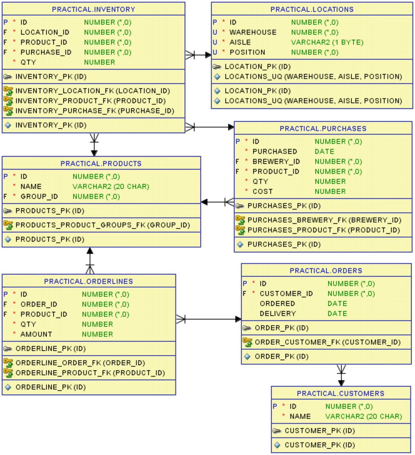
When you look at Figure 13-1, there are a lot of tables, mostly to show you a fairly realistic data model. For demonstration purposes, I could have simplified this a lot, but I will do that with a view, as you’ll see shortly.
Figure 13-1
The tables used in this chapter
In the inventory table is stored how many of a given product are currently stored in a given location and from which purchase did that quantity originate (thereby giving us the age of quantity in that location). Basically that’s just foreign keys to locations, products, and purchases tables and then a qty column.
Then there are customers who have given orders that have orderlines specifying which products they are buying, how many, and for how much.
To simplify working with these tables, I create the view inventory_with_dims shown in Listing 13-1. This simply joins the inventory table with the three referenced tables, so that I have all relevant information (product name, purchase date, warehouse, aisle, position) for each inventory row.
create or replace view inventory_with_dims
as
select
i.id
, i.product_id
, p.name as product_name
, i.purchase_id
, pu.purchased
, i.location_id
, l.warehouse
, l.aisle
, l.position
, i.qty
from inventory i
join purchases pu
on pu.id = i.purchase_id
join products p
on p.id = i.product_id
join locations l
on l.id = i.location_id;
Listing 13-1
View joining inventory with other relevant tables
When I build my picking SQL statement, I’ll be using this view together with the orderlines table.
Building the picking SQL
For the first two parts of the problem, I will just pick a single order, the order with id = 421. In Listing 13-2, I’ll just show you the data of that order.
SQL> select
2 c.id as c_id
3 , c.name as c_name
4 , o.id as o_id
5 , ol.product_id as p_id
6 , p.name as p_name
7 , ol.qty
8 from orders o
9 join orderlines ol
10 on ol.order_id = o.id
11 join products p
12 on p.id = ol.product_id
13 join customers c
14 on c.id = o.customer_id
15 where o.id = 421
16 order by o.id, ol.product_id;
Listing 13-2
Data for the order I am going to pick
As you see here in the output, the White Hart pub has ordered 110 of Hoppy Crude Oil and 140 of Der Helle Kumpel:
C_ID C_NAME O_ID P_ID P_NAME QTY
50042 The White Hart 421 4280 Hoppy Crude Oil 110
50042 The White Hart 421 6520 Der Helle Kumpel 140
Then it’s time to start building an analytic SQL statement.
Solving picking an order by FIFO
The first thing I do is I join the orderlines of order 421 with the inventory_with_dims view in Listing 13-3.
(Bear with me that I’m using very short column aliases, but it’s an easy way to get a sqlcl output with very narrow columns that fits nicely on print.)
SQL> select
2 i.product_id as p_id
3 , ol.qty as ord_q
4 , i.qty as loc_q
5 , sum(i.qty) over (
6 partition by i.product_id
7 order by i.purchased, i.qty
8 rows between unbounded preceding and current row
9 ) as acc_q
10 , i.purchased
11 , i.warehouse as wh
12 , i.aisle as ai
13 , i.position as pos
14 from orderlines ol
15 join inventory_with_dims i
16 on i.product_id = ol.product_id
17 where ol.order_id = 421
18 order by i.product_id, i.purchased, i.qty;
Listing 13-3
Possible inventory to pick – in order of purchase date
In lines 5–9 I am doing a rolling sum of the inventory quantity, partitioned by product and ordered by purchase date. And for those cases with multiple rows having the same purchase date, I add the quantity to the ordering, so I get to clean out smaller quantities in the warehouse first.
In this query, the final order by in line 18 matches the columns of the partition by followed by order by in the analytic function. This is not necessary (later I will change this on purpose), but when they match like here, then the optimizer can do both with a single sorting operation.
The output shows me for each of the two ordered products all of the inventory in purchase order, and in column acc_q (accumulated quantity), I can see the rolling sum:
P_ID ORD_Q LOC_Q ACC_Q PURCHASED WH AI POS
4280 110 36 36 2018-02-23 1 C 1
4280 110 39 75 2018-04-23 1 D 18
4280 110 35 110 2018-06-23 2 B 3
4280 110 34 144 2018-08-23 2 C 20
4280 110 37 181 2018-10-23 1 A 4
4280 110 19 200 2018-12-23 2 C 7
6520 140 14 14 2018-02-26 2 B 5
6520 140 14 28 2018-02-26 1 A 29
6520 140 20 48 2018-02-26 1 C 13
6520 140 24 72 2018-02-26 2 B 26
6520 140 26 98 2018-04-26 2 D 9
6520 140 48 146 2018-04-26 1 A 16
6520 140 70 216 2018-06-26 1 C 5
6520 140 21 237 2018-08-26 2 C 31
6520 140 48 285 2018-08-26 1 D 19
6520 140 72 357 2018-10-26 2 A 1
6520 140 43 400 2018-12-26 1 B 32
So this looks just like what I need, right? When the rolling sum is larger than the ordered quantity, I’ve got enough, right? I’m going to try that in Listing 13-4 by wrapping Listing 13-3 in an inline view and filtering in the where clause.
SQL> select *
2 from (
...
20 )
21 where acc_q <= ord_q
22 order by p_id, purchased, loc_q;
Listing 13-4
Filtering on the accumulated sum
Did I get the right result? No, not quite:
P_ID ORD_Q LOC_Q ACC_Q PURCHASED WH AI POS
4280 110 36 36 2018-02-23 1 C 1
4280 110 39 75 2018-04-23 1 D 18
4280 110 35 110 2018-06-23 2 B 3
6520 140 14 14 2018-02-26 2 B 5
6520 140 14 28 2018-02-26 1 A 29
6520 140 20 48 2018-02-26 1 C 13
6520 140 24 72 2018-02-26 2 B 26
6520 140 26 98 2018-04-26 2 D 9
Product 4280 is OK; it just happens that the rolling sum exactly matches the ordered quantity of 110 after picking at three locations. But product 6520 only gets to pick 98, where it should get 140? If you look back at the previous output, you’ll see that by the next location (1 A 16), the rolling sum becomes 146, which is greater than 140 so that row is not included in the output, even though I need to pick most of the quantity of that location.
The problem is that I cannot in the where clause create a filter that will include the first row where the rolling sum is greater than the ordered quantity, but not any more rows than that.
But what I can do is to create a rolling sum that accumulates the previous rows only, rather than including the current row. This is simply done in Listing 13-5 by simply changing the window end point of Listing 13-3 from current row to 1 preceding in line 8.
...
5 , sum(i.qty) over (
6 partition by i.product_id
7 order by i.purchased, i.qty
8 rows between unbounded preceding and 1 preceding
9 ) as acc_prv_q
...
Listing 13-5
Accumulated sum of only the previous rows
The rolling sums in this output is pushed one row down when compared to the output of Listing 13-3:
P_ID ORD_Q LOC_Q ACC_PRV_Q PURCHASED WH AI POS
4280 110 36 2018-02-23 1 C 1
4280 110 39 36 2018-04-23 1 D 18
4280 110 35 75 2018-06-23 2 B 3
4280 110 34 110 2018-08-23 2 C 20
4280 110 37 144 2018-10-23 1 A 4
4280 110 19 181 2018-12-23 2 C 7
6520 140 14 2018-02-26 2 B 5
6520 140 14 14 2018-02-26 1 A 29
6520 140 20 28 2018-02-26 1 C 13
6520 140 24 48 2018-02-26 2 B 26
6520 140 26 72 2018-04-26 2 D 9
6520 140 48 98 2018-04-26 1 A 16
6520 140 70 146 2018-06-26 1 C 5
6520 140 21 216 2018-08-26 2 C 31
6520 140 48 237 2018-08-26 1 D 19
6520 140 72 285 2018-10-26 2 A 1
6520 140 43 357 2018-12-26 1 B 32
This means that the row of product 6520 in location 1 A 16 that was missing in the output of Listing 13-4 is now within the window of rows where acc_prv_q is less than ord_q, so I can create Listing 13-6 that correctly filters what I need. It is the solution to the first problem of the three described at the beginning of the chapter.
SQL> select
2 wh, ai, pos, p_id
3 , least(loc_q, ord_q - acc_prv_q) as pick_q
4 from (
5 select
6 i.product_id as p_id
7 , ol.qty as ord_q
8 , i.qty as loc_q
9 , nvl(sum(i.qty) over (
10 partition by i.product_id
11 order by i.purchased, i.qty
12 rows between unbounded preceding and 1 preceding
13 ), 0) as acc_prv_q
14 , i.purchased
15 , i.warehouse as wh
16 , i.aisle as ai
17 , i.position as pos
18 from orderlines ol
19 join inventory_with_dims i
20 on i.product_id = ol.product_id
21 where ol.order_id = 421
22 )
23 where acc_prv_q < ord_q
24 order by wh, ai, pos;
Listing 13-6
Filtering on the accumulation of previous rows
In lines 9–13, I do the rolling sum of previous rows, but note that I need to use nvl to turn the null of the first row into a zero – otherwise, the where clause in line 23 will fail.
That where clause you can read as “As long as the previous row(s) have not yet picked enough to fulfill the order, I need to include this row in the output.”
In line 3, I calculate how much needs to be picked at the location of each row. I know how much still needs to be picked; it’s the ordered quantity (ord_q) minus what has already been picked in the previous rows (acc_prv_q). If this is smaller than what is on the location (loc_q), that is what I need to pick. But if it is greater, then of course I can only pick as much as is on the location. In other words, I need to pick the smaller of the two numbers, which I can do with the least function.
Finally I’ve cleaned up the select list only saving what’s necessary to put on the picking list, and in line 23, I’m ordering the rows in location order:
WH AI POS P_ID PICK_Q
1 A 16 6520 42
1 A 29 6520 14
1 C 1 4280 36
1 C 13 6520 20
1 D 18 4280 39
2 B 3 4280 35
2 B 5 6520 14
2 B 26 6520 24
2 D 9 6520 26
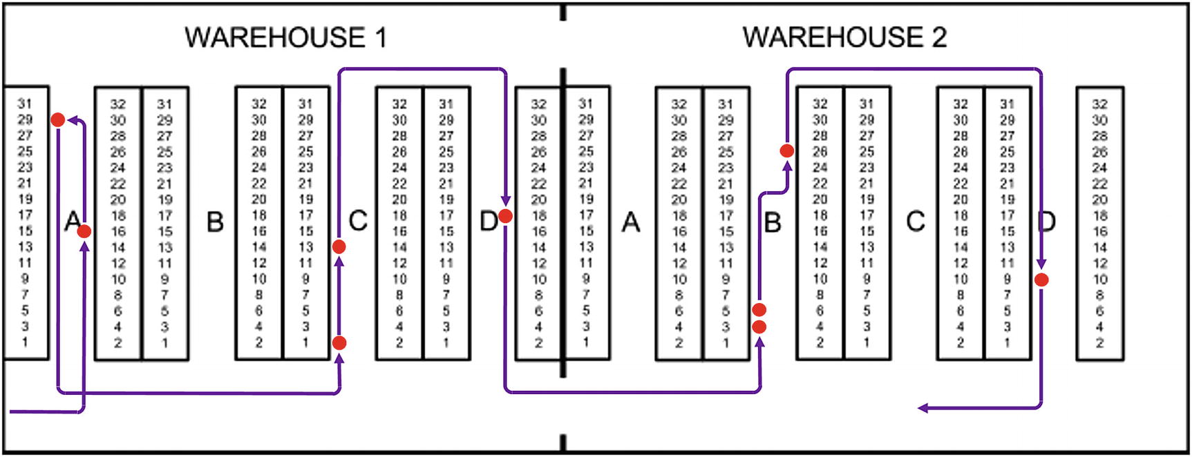
The picking operator can now take this list and drive around the warehouse picking the goods as specified. He’ll follow the route shown in Figure 13-2.
Figure 13-2
The result of the first version of the FIFO picking query
This route has the problem that after having picked the first two locations in aisle A, he needs to start “from the bottom” in aisle C. That means he either has to turn around (as shown in the figure) or he could take an unnecessary drive “down” aisle B. Neither is really satisfactory, and I’ll come back to the solution of this in a little while.
Easy switch of picking principle
But first I’d like to stress the point that the order by of the query itself and the order by within the analytic function do not have to be identical, as they were in Listing 13-3; they can be different like in the picking list query of Listing 13-6, where I use this fact to select the inventory in FIFO order with the analytic orderby, but give the output of the selected rows in location order.
This separation means that I can easily switch picking principle simply by changing my analytic order by, but still get an output in location order.
So for these examples, imagine that beers can keep indefinitely, so it does not matter if I use the first-in, first-out principle or not.
I could then use a picking principle saying that I want to prioritize locations close to the starting point of the driver to give him a short picking route. I just need to change line 11 in Listing 13-6:
...
11 order by i.warehouse, i.aisle, i.position
...
Selecting inventory to pick in location order gives a short route; he does not have to enter warehouse 2 at all:
WH AI POS P_ID PICK_Q
1 A 4 4280 37
1 A 16 6520 48
1 A 29 6520 14
1 B 32 6520 43
1 C 1 4280 36
1 C 5 6520 35
1 D 18 4280 37
Or I could use as picking principle that I want the smallest number of picks:
...
11 order by i.qty desc
...
This will pick from inventories with large quantities first, making it possible to fulfill the order with just five picks:
WH AI POS P_ID PICK_Q
1 A 4 4280 37
1 C 1 4280 34
1 C 5 6520 68
1 D 18 4280 39
2 A 1 6520 72
But if I pick from large quantities first, then over time the warehouse will be full of locations that have just a small quantity that was “left over” from previous picks. I could choose a picking principle that will clean up such small quantities, freeing the locations for new inventory:
...
11 order by i.qty
...
Ordering by quantity ascending instead of descending helps cleaning out locations in the warehouse, but of course then the operator has to pick in more places:
WH AI POS P_ID PICK_Q
1 A 29 6520 14
1 B 32 6520 21
1 C 1 4280 22
1 C 13 6520 20
2 B 3 4280 35
2 B 5 6520 14
2 B 26 6520 24
2 C 7 4280 19
2 C 20 4280 34
2 C 31 6520 21
2 D 9 6520 26
As you can see, having separated the order by that selects the inventory from the order by that controls the picking order, it is easy to switch picking strategies.
With that point made, back to solving the routing problem of Figure 13-2.
Solving optimal picking route
Simply ordering the output in location order means the picking operator needs to drive in the same direction (“upward”) in every aisle – this is not optimal. I’d like him to switch directions so that every other aisle he drives “down.”
But it is not so simple that I can just say up in aisle A and C, down in aisle B and D. Instead I need it to be up in the first, third, fifth…aisle he visits and then down in the second, fourth, sixth…aisle he visits.
To do that, I start by expanding Listing 13-6 with an extra column giving each visited aisle a consecutive number (Listing 13-7).
SQL> select
2 wh, ai
3 , dense_rank() over (
4 order by wh, ai
5 ) as ai#
6 , pos, p_id
7 , least(loc_q, ord_q - acc_prv_q) as pick_q
8 from (
...
26 )
27 where acc_prv_q < ord_q
28 order by wh, ai, pos;
Listing 13-7
Consecutively numbering visited warehouse aisles
The analytic function dense_rank in lines 3–5 gives the same rank to rows that have the same value in the columns used in the order by. And unlike rank, dense_rank does not skip any numbers (as I showed in Chapter 12); it assigns the ranks consecutively.
So using warehouse and aisle in the order by in dense_rank, the ai# column contains the “visited aisle number” I want:
WH AI AI# POS P_ID PICK_Q
1 A 1 16 6520 42
1 A 1 29 6520 14
1 C 2 1 4280 36
1 C 2 13 6520 20
1 D 3 18 4280 39
2 B 4 3 4280 35
2 B 4 5 6520 14
2 B 4 26 6520 24
2 D 5 9 6520 26
That enables me to wrap Listing 13-7 in an inline view to create Listing 13-8 with an odd-even ordering logic.
SQL> select *
2 from (
...
30 )
31 order by
32 wh, ai#
33 , case
34 when mod(ai#, 2) = 1 then +pos
35 else -pos
36 end;
Listing 13-8
Ordering ascending and descending alternately
First, I order by warehouse and visited aisle, but then within each aisle, I use the case structure in lines 33–36 to order the positions ascending in odd numbered aisles and descending in even numbered aisles:
WH AI AI# POS P_ID PICK_Q
1 A 1 16 6520 42
1 A 1 29 6520 14
1 C 2 13 6520 20
1 C 2 1 4280 36
1 D 3 18 4280 39
2 B 4 26 6520 24
2 B 4 5 6520 14
2 B 4 3 4280 35
2 D 5 9 6520 26
That gives the operator a better picking route as you can see in Figure 13-3, so Listing 13-8 is the solution to the second of my three problems.
Figure 13-3
Alternating position order of odd/even visited aisles
Again I can show a variation where I can adapt the query very easily to match changing conditions. In Figure 13-3, you see a door between warehouses 1 and 2 both at the bottom and at the top, but what happens if there’s only a door at the bottom and it’s closed at the top?
A small change to the dense_rank call of Listing 13-8 produces Listing 13-9.
...
5 , dense_rank() over (
6 partition by wh
7 order by ai
8 ) as ai#
...
Listing 13-9
Restarting aisle numbering within each warehouse
All I’ve done is to change an order by warehouse and aisle into a partition by warehouse and order by aisle. The result is that the ranks assigned in column ai# restart from 1 in each warehouse:
WH AI AI# POS P_ID PICK_Q
1 A 1 16 6520 42
1 A 1 29 6520 14
1 C 2 13 6520 20
1 C 2 1 4280 36
1 D 3 18 4280 39
2 B 1 3 4280 35
2 B 1 5 6520 14
2 B 1 26 6520 24
2 D 2 9 6520 26
When ai# restarts in each warehouse, that means that aisle B in warehouse 2 changes from being the fourth aisle he visits overall to being the first aisle he visits in warehouse 2. That means it changes from being an even numbered aisle (ordered descending) to being an odd numbered aisle (ordered ascending).
And that gives the picking route shown in Figure 13-4.
Figure 13-4
What happens when there is just one door between warehouses
The first two problems are now solved, so I’ll now move on to the third and last problem.
Solving batch picking
It’s all well and good that I now can pick a single order by FIFO with a good picking route, but to work efficiently, I need the picking operator to be able to pick multiple orders simultaneously in a single drive through the warehouses.
So I’m going to use Listing 13-2 again to show order data, just this time for two other orders. In real life, I’d probably model a “picking batch” table to use for specifying which orders are to be included in a batch, but here I’m just coding the two order ids using in:
...
15 where o.id in (422, 423)
...
And it shows me two pubs that each have ordered a quantity of both Hoppy Crude Oil and Der Helle Kumpel:
C_ID C_NAME O_ID P_ID P_NAME QTY
51069 Der Wichtelmann 422 4280 Hoppy Crude Oil 80
51069 Der Wichtelmann 422 6520 Der Helle Kumpel 80
50741 Hygge og Humle 423 4280 Hoppy Crude Oil 60
50741 Hygge og Humle 423 6520 Der Helle Kumpel 40
I can start simple in Listing 13-10 by just finding the total quantities ordered for each product and then applying the FIFO picking method of Listing 13-6 to those totals.
SQL> with orderbatch as (
2 select
3 ol.product_id
4 , sum(ol.qty) as qty
5 from orderlines ol
6 where ol.order_id in (422, 423)
7 group by ol.product_id
8 )
9 select
10 wh, ai, pos, p_id
11 , least(loc_q, ord_q - acc_prv_q) as pick_q
12 from (
13 select
14 i.product_id as p_id
15 , ob.qty as ord_q
16 , i.qty as loc_q
17 , nvl(sum(i.qty) over (
18 partition by i.product_id
19 order by i.purchased, i.qty
20 rows between unbounded preceding and 1 preceding
21 ), 0) as acc_prv_q
22 , i.purchased
23 , i.warehouse as wh
24 , i.aisle as ai
25 , i.position as pos
26 from orderbatch ob
27 join inventory_with_dims i
28 on i.product_id = ob.product_id
29 )
30 where acc_prv_q < ord_q
31 order by wh, ai, pos;
Listing 13-10
FIFO picking of the total quantities
Using the with clause, I create the orderbatch subquery in lines 1–8 that simply is an aggregation of the ordered quantities per product. The rest of the query is identical to Listing 13-6, except that it uses orderbatch in line 26 instead of table orderlines.
The output is a picking list showing what needs to be picked to fulfill the two orders:
WH AI POS P_ID PICK_Q
1 A 16 6520 22
1 A 29 6520 14
1 C 1 4280 36
1 C 13 6520 20
1 D 18 4280 39
2 B 3 4280 35
2 B 5 6520 14
2 B 26 6520 24
2 C 20 4280 30
2 D 9 6520 26
But there’s a slight problem for the picking operator – he can see how much to pick, but not how much of that he needs to pack in each order.
To figure that out, I need to calculate some quantity intervals in Listing 13-11.
SQL> with orderbatch as (
...
8 )
9 select
10 wh, ai, pos, p_id
11 , least(loc_q, ord_q - acc_prv_q) as pick_q
12 , acc_prv_q + 1 as from_q
13 , least(acc_q, ord_q) as to_q
14 from (
15 select
16 i.product_id as p_id
17 , ob.qty as ord_q
18 , i.qty as loc_q
19 , nvl(sum(i.qty) over (
20 partition by i.product_id
21 order by i.purchased, i.qty
22 rows between unbounded preceding and 1 preceding
23 ), 0) as acc_prv_q
24 , nvl(sum(i.qty) over (
25 partition by i.product_id
26 order by i.purchased, i.qty
27 rows between unbounded preceding and current row
28 ), 0) as acc_q
29 , i.purchased
30 , i.warehouse as wh
31 , i.aisle as ai
32 , i.position as pos
33 from orderbatch ob
34 join inventory_with_dims i
35 on i.product_id = ob.product_id
36 )
37 where acc_prv_q < ord_q
38 order by p_id, purchased, loc_q, wh, ai, pos;
Listing 13-11
Quantity intervals for each pick out of total per product
The inline view in lines 14–36 is almost the same as before, but I have added an extra rolling sum in lines 24–28, so I now have both a rolling sum of the previous rows in acc_prv_q and a rolling sum that includes the current row in acc_q.
With those I can in lines 12–13 calculate the from and to quantity intervals for the row, showing you this output that I’ve ordered in line 38 so that you easily can see what happens with the intervals:
WH AI POS P_ID PICK_Q FROM_Q TO_Q
1 C 1 4280 36 1 36
1 D 18 4280 39 37 75
2 B 3 4280 35 76 110
2 C 20 4280 30 111 140
1 A 29 6520 14 1 14
2 B 5 6520 14 15 28
1 C 13 6520 20 29 48
2 B 26 6520 24 49 72
2 D 9 6520 26 73 98
1 A 16 6520 22 99 120
With these quantity intervals, you can read that the 36 to be picked in the first row are numbers 1-36 out of the total 140 to be picked of product 4280, the 39 in the next row are then numbers 37-75 out of the 140, and so on.
If you’ve a keen eye, you may have spotted that in Listing 13-11, I am actually doing a superfluous analytic function call, since I am using a call both to calculate rolling sum of previous rows and to calculate rolling sum including the current row. But the latter could also be calculated as the rolling sum of previous rows + the quantity in the current row.
So in Listing 13-12, I’ve changed slightly to only do the rolling sum of previous rows in order to save an analytic function call.
SQL> with orderbatch as (
...
8 )
9 select
10 wh, ai, pos, p_id
11 , least(loc_q, ord_q - acc_prv_q) as pick_q
12 , acc_prv_q + 1 as from_q
13 , least(acc_prv_q + loc_q, ord_q) as to_q
14 from (
15 select
16 i.product_id as p_id
17 , ob.qty as ord_q
18 , i.qty as loc_q
19 , nvl(sum(i.qty) over (
20 partition by i.product_id
21 order by i.purchased, i.qty
22 rows between unbounded preceding and 1 preceding
23 ), 0) as acc_prv_q
24 , i.purchased
25 , i.warehouse as wh
26 , i.aisle as ai
27 , i.position as pos
28 from orderbatch ob
29 join inventory_with_dims i
30 on i.product_id = ob.product_id
31 )
32 where acc_prv_q < ord_q
33 order by p_id, purchased, loc_q, wh, ai, pos;
Listing 13-12
Quantity intervals with a single analytic sum
The inline view again only contains the acc_prv_q (as it used to), and then in line 13, I am using acc_prv_q + loc_q instead of the acc_q I no longer have. The result of Listing 13-12 is identical to that of Listing 13-11.
Having quantity intervals for the picks is not enough; I also need similar quantity intervals for the orders, as I show in Listing 13-13.
SQL> select
2 ol.order_id as o_id
3 , ol.product_id as p_id
4 , ol.qty
5 , nvl(sum(ol.qty) over (
6 partition by ol.product_id
7 order by ol.order_id
8 rows between unbounded preceding and 1 preceding
9 ), 0) + 1 as from_q
10 , nvl(sum(ol.qty) over (
11 partition by ol.product_id
12 order by ol.order_id
13 rows between unbounded preceding and 1 preceding
14 ), 0) + ol.qty as to_q
15 from orderlines ol
16 where ol.order_id in (422, 423)
17 order by ol.product_id, ol.order_id;
Listing 13-13
Quantity intervals for each order out of total per product
I’m skipping the inline view here and instead calculate from_q directly in lines 5–9 and to_q in lines 10–14. In both calculations, I’m doing a rolling sum of all previous rows, so that when I’m using the exact same analytic function expression twice, the SQL engine will recognize this and only perform the analytic call once.
The output shows me then that the 80 of product 4280 that is ordered in order 422 are numbers 1-80 out of the 140, just like the picking quantity intervals before.
O_ID P_ID QTY FROM_Q TO_Q
422 4280 80 1 80
423 4280 60 81 140
422 6520 80 1 80
423 6520 40 81 120
With the two sets of quantity intervals, I can join them where they overlap and that way see how many of each pick go to what order. Listing 13-14 brings the code together.
SQL> with olines as (
2 select
3 ol.order_id as o_id
4 , ol.product_id as p_id
5 , ol.qty
6 , nvl(sum(ol.qty) over (
7 partition by ol.product_id
8 order by ol.order_id
9 rows between unbounded preceding and 1 preceding
10 ), 0) + 1 as from_q
11 , nvl(sum(ol.qty) over (
12 partition by ol.product_id
13 order by ol.order_id
14 rows between unbounded preceding and 1 preceding
15 ), 0) + ol.qty as to_q
16 from orderlines ol
17 where ol.order_id in (422, 423)
18 ), orderbatch as (
19 select
20 ol.p_id
21 , sum(ol.qty) as qty
22 from olines ol
23 group by ol.p_id
24 ), fifo as (
25 select
26 wh, ai, pos, p_id, loc_q
27 , least(loc_q, ord_q - acc_prv_q) as pick_q
28 , acc_prv_q + 1 as from_q
29 , least(acc_prv_q + loc_q, ord_q) as to_q
30 from (
31 select
32 i.product_id as p_id
33 , ob.qty as ord_q
34 , i.qty as loc_q
35 , nvl(sum(i.qty) over (
36 partition by i.product_id
37 order by i.purchased, i.qty
38 rows between unbounded preceding and 1 preceding
39 ), 0) as acc_prv_q
40 , i.purchased
41 , i.warehouse as wh
42 , i.aisle as ai
43 , i.position as pos
44 from orderbatch ob
45 join inventory_with_dims i
46 on i.product_id = ob.p_id
47 )
48 where acc_prv_q < ord_q
49 )
50 select
51 f.wh, f.ai, f.pos, f.p_id
52 , f.pick_q, f.from_q as p_f_q, f.to_q as p_t_q
53 , o.o_id , o.from_q as o_f_q, o.to_q as o_t_q
54 from fifo f
55 join olines o
56 on o.p_id = f.p_id
57 and o.to_q >= f.from_q
58 and o.from_q <= f.to_q
59 order by f.p_id, f.from_q, o.from_q;
Listing 13-14
Join overlapping pick and order quantity intervals
I build the query using three withclause subqueries:
First I create olines, which is Listing 13-13 calculating the quantity intervals for the orderlines.
Then orderbatch, similar to how I did it in Listing 13-12, except that I do the aggregation using olines in line 22 instead of the orderlines table, since olines already has the desired orderlines.
The third subquery is fifo, which also comes from Listing 13-12 and takes care of building the FIFO picks including quantity intervals.
The main query then is a join of fifo and olines on the product id and on overlapping quantity intervals. In the resulting output, you see the from/to intervals for the picks as p_f_q/p_t_q and for the orderlines as o_f_q/o_t_q (short column names are good for print):
WH AI POS P_ID PICK_Q P_F_Q P_T_Q O_ID O_F_Q O_T_Q
1 C 1 4280 36 1 36 422 1 80
1 D 18 4280 39 37 75 422 1 80
2 B 3 4280 35 76 110 422 1 80
2 B 3 4280 35 76 110 423 81 140
2 C 20 4280 30 111 140 423 81 140
1 A 29 6520 14 1 14 422 1 80
2 B 5 6520 14 15 28 422 1 80
1 C 13 6520 20 29 48 422 1 80
2 B 26 6520 24 49 72 422 1 80
2 D 9 6520 26 73 98 422 1 80
2 D 9 6520 26 73 98 423 81 120
1 A 16 6520 22 99 120 423 81 120
In the first row, all 36 go to order 422. Likewise in the second row, all 39 go to order 422.
But the next 35 picked are numbers 76-110 (out of 140), which overlaps both with order 422 (numbers 1-80) and order 423 (numbers 81-140). You can see from those overlaps that 5 of the 35 (numbers 76-80) should go to order 422 and the 30 of the 35 (numbers 81-110) should go to order 423.
In Listing 13-15, I calculate this as well as clean up the query a bit to not show the intermediate calculation columns.
How much quantity from each pick goes to which order
Lines 53–56 calculate the “quantity for order” (q_f_o) by taking either the quantity that is on the location or the “size of the interval overlap,” whichever is the smaller of the two. The result is this output with all the necessary information for the picking operator:
WH AI POS P_ID PICK_Q O_ID Q_F_O
1 C 1 4280 36 422 36
1 D 18 4280 39 422 39
2 B 3 4280 35 422 5
2 B 3 4280 35 423 30
2 C 20 4280 30 423 30
1 A 29 6520 14 422 14
2 B 5 6520 14 422 14
1 C 13 6520 20 422 20
2 B 26 6520 24 422 24
2 D 9 6520 26 422 8
2 D 9 6520 26 423 18
1 A 16 6520 22 423 22
That solved the third problem; now all that is needed to complete the solution is to combine the solutions of problems 2 and 3, so the picking operator also can do the batch picking in an efficient picking route.
Finalizing the complete picking SQL
I have Listing 13-15 for batch picking and Listing 13-8 for a good picking route. Combining the two in Listing 13-16 gives me the complete solution.
The with clause subqueries olines, orderbatch, and fifo are the same as Listing 13-15. Then the main query from Listing 13-15 I have put into subquery pick in lines 49–66.
I’ve added the calculation of the “visited aisle number” ai# (from Listing 13-8) in lines 52–54.
Then the main query is simply selecting the necessary information from the pick subquery and using the order by from Listing 13-8 to give an optimal picking route:
WH AI POS P_ID PICK_Q O_ID Q_F_O
1 A 16 6520 22 423 22
1 A 29 6520 14 422 14
1 C 13 6520 20 422 20
1 C 1 4280 36 422 36
1 D 18 4280 39 422 39
2 B 26 6520 24 422 24
2 B 5 6520 14 422 14
2 B 3 4280 35 422 5
2 B 3 4280 35 423 30
2 C 20 4280 30 423 30
2 D 9 6520 26 422 8
2 D 9 6520 26 423 18
Where a location is repeated on the list, like 2 B 3, you can see that it shows 35 should be picked, 5 of which are to be placed in the package for order 422 and 30 are for the package for order 423.
With this list, the picking operator will be led in a good route through the warehouses, picking products for a batch of multiple orders, where the products have been selected by the first-in, first-out principle.
In total this is practically a complete warehouse goods picking app in a single SQL statement.
Lessons learned
This chapter has shown you the building of a single SQL app with multiple uses of analytic functions that have given you knowledge on
Using the window clause to apply analytic sum to a subset of the rows to find the subset that gives a sufficiently large result
Calculating intervals with analytic rolling sums to find overlapping intervals
Assigning dense_rank to results for alternating ascending and descending ordering
When you understand how to build a statement like this piece by piece with analytic functions, you can create many similar statements that contain a lot of business logic, thereby achieving an app with a lot better performance than extracting the data and doing the same logic procedurally.