CHAPTER 6

PivotTables

PivotTables are a neat feature of Excel 2007 that allows users to summarize and analyze data. By adding or removing data elements from an onscreen selection tool, your users can easily reshape their data for analysis or reporting.

A PivotTable report provides an interactive method to quickly and easily summarize large amounts of data (without the need to export the data to an external database system like Microsoft Access or an external reporting tool).

Here are some examples of when you might want to use a PivotTable to display your data:

• To query large amounts of data and create different views
• To aggregate and subtotal data, and/or create custom calculations and formulas
• To expand and collapse levels of data
• To move rows to columns or columns to rows to see different summaries of the source data (hence the term pivot)

PivotTables enable you to take huge amounts of data and present a concise, easy-to-read view of that data.

Putting Data into a PivotTable Report

In the Download section for this book on the Apress web site, find the file named PivotTable01.xlsx and open it.

Remember our fictitious band "VBA" from Chapter 1? Well, they've been out touring and their manager wants to see what's selling and what's not, and where items are selling best. PivotTable01.xlsx contains sales data from the first quarter of their tour, as shown in Figure 6-1.

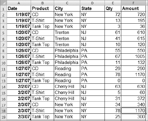
Figure 6-1. Tour sales data

A good way for the manager to look at this data is via an Excel 2007 PivotTable report. We're going to record a macro while we create a PivotTable. Then we'll take a look at some of the properties and methods available to us.

1. Start the Macro Recorder (Developer ribbon Record Macro).
2. Name the new macro MakePivotTable.
3. Put the cursor anywhere inside the sales data.
4. Choose Insert Ribbon Tables PivotTable. The Create PivotTable dialog box will be displayed, as shown in Figure 6-2.
   
   
   

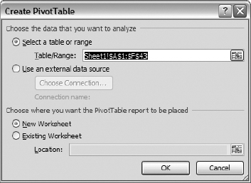
   Figure 6-2. Create PivotTable dialog box

The Create PivotTable dialog box contains two sections. The first section is where you can choose a data source. This can be a table or range within an Excel workbook or data from an external source. External data is accessed through a connection file, such as an Office Data Connection (ODC) file (.odc) or a Universal Data Connection (UDC) file (.udcx).

The second section lets you dictate where you would like the PivotTable report to be placed.

1. For now, just accept the defaults and click OK. A blank PivotTable report will be inserted on Sheet4, as shown in Figure 6-3.

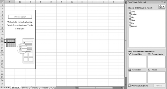
Figure 6-3. Excel 2007 PivotTable report default view

The new PivotTable report has a revamped interface that allows for easy manipulation of pivot data. All fields in the table are listed in the PivotTable Field List pane, which you can see on the right side of Figure 6-3. Check boxes are provided for users to choose the fields they want to include in the report. Text fields will by default place themselves in the Row Labels list and numeric fields will default to the Values list.

An easier way to create a report is to drag the field from the selection section at the top of the PivotTable Field List pane to the correct list below (shown in Figure 6-4).

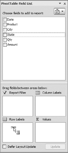
Figure 6-4. Dragging the State field to the Row Labels section

Once you drop the field, the PivotTable updates to show the text or data (when available), as shown in Figure 6-5.

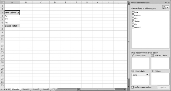
Figure 6-5. State field added to the PivotTable

1. Drag the Product field to the Column Labels list.
2. Drag the Qty field to the Values list. The PivotTable Field List pane should look like Figure 6-6.
   
   
   

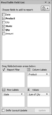
   Figure 6-6. PivotTable Field List with all fields added

The PivotTable report will look like Figure 6-7.

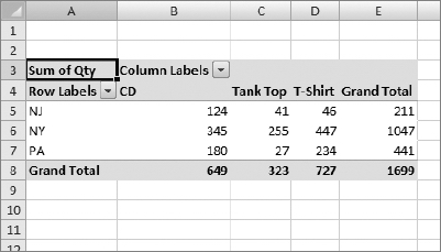
Figure 6-7. The completed PivotTable report

We see a sales summary by product line by state. But what if we also need to see sales by city within each state?

1. Drag the City field to the Row Labels list and place it under the State field.

The finished report should now look like Figure 6-8.

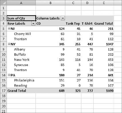
Figure 6-8. City added to PivotTable report

1. Stop the Macro Recorder by clicking the Stop Recording command on the Developer ribbon.

If you have had any experience with previous versions of Excel PivotTable reports, you probably immediately noticed a change in the UI of the blank PivotTable.

The PivotTable Field List pane in Excel 2007 now does the work of all three components shown in Figure 6-9. The user experience is much cleaner this way, and makes using –PivotTables much easier for users.

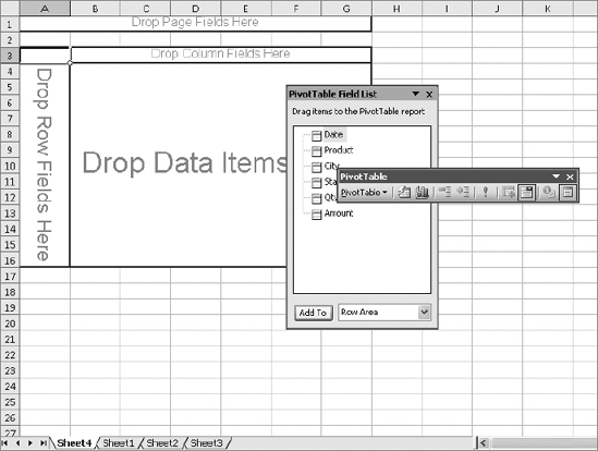
Figure 6-9. Excel 2003 PivotTable report default view

The Macro Code

Listing 6-1 shows the code the Macro Recorder generated for us.

The first thing the code does is add a new worksheet to the workbook. Then it creates the PivotTable using the source data range we provided in the Create PivotTable dialog box. Then it places the PivotTable on the new sheet (in this case Sheet4) and gives it a default name.

Sheets.Add
ActiveWorkbook.PivotCaches.Create(SourceType:=xlDatabase, SourceData:=
    "Sheet1!R1C1:R43C6", Version:=xlPivotTableVersion12).CreatePivotTable
    TableDestination:="Sheet4!R3C1", TableName:="PivotTable1", DefaultVersion
    :=xlPivotTableVersion12

The PivotCaches.Create method takes three arguments, of which only one (SourceType) is required. The SourceData argument is required when SourceType does not equal xlExternal. Table 6-1 lists the PivotCaches.Create method's arguments and describes them.

Table 6-1. PivotCaches.Create Method Arguments

Name	Required (Y/N)	Data Type	Description
SourceType	Y	xlPivotTableSourceType	Choices are xlConsolidation, xlDatabase, or xlExternal
SourceData	N	Variant	The data for the new PivotTable cache
Version	N	Variant	Version of the PivotTable

The PivotCaches.Create method returns a PivotCache object. The Macro Recorder very cleverly calls the CreatePivotTable method based on the return from the Create method in one long (but readable) line of code:

ActiveWorkbook.PivotCaches.Create(SourceType:=xlDatabase, SourceData:=
    "Sheet1!R1C1:R43C6", Version:=xlPivotTableVersion12).CreatePivotTable
    TableDestination:="Sheet4!R3C1", TableName:="PivotTable1", DefaultVersion
    :=xlPivotTableVersion12

The CreatePivotTable method defines where the table will be placed, its name, and its default version. Table 6-2 lists the CreatePivotTable method's arguments.

Table 6-2. CreatePivotTable Method Arguments

Name	Required (Y/N)	Data Type	Description
TableDestination	Y	Variant	The cell in the top-left corner of the PivotTable's destination range.
TableName	N	Variant	The name of the PivotTable report.
ReadData	N	Variant	Set to True to create a PivotTable cache that contains all of the records from the data source (can be very large). Set to False to enable setting some fields as server-based page fields before the data is read.
DefaultVersion	N	Variant	The default version of the PivotTable report.

The code then selects the new sheet and the starting range location for the PivotTable.

Sheets("Sheet4").Select
Cells(3, 1).Select

We added two text fields (State and Products) to the PivotTable Field List pane and one data field containing the item quantities (Qty):

With ActiveSheet.PivotTables("PivotTable1").PivotFields("State")
    .Orientation = xlRowField
    .Position = 1
End With
With ActiveSheet.PivotTables("PivotTable1").PivotFields("Product")
    .Orientation = xlColumnField
    .Position = 1
End With
ActiveSheet.PivotTables("PivotTable1").AddDataField ActiveSheet.PivotTables(
    "PivotTable1").PivotFields("Qty"), "Sum of Qty", xlSum

This is where the code is telling the PivotTable how to display the data assigned to each PivotField object. The Orientation property is set to a value of the xlPivotFieldOrientation enumeration type, as shown in Table 6-3.

Table 6-3. xlPivotFieldOrientation Enumerations

Name	Value	Description
xlRowField	1	Row
xlColumnField	2	Column
xlPageField	3	Page
xlDataField	4	Data
xlHidden	0	Hidden

The Position property notes where in the row or column hierarchy the field belongs, and therefore how the data will be grouped on the PivotTable. After we added the City field to the Row Labels list in the PivotTable Field List pane, the next bit of code was added:

With ActiveSheet.PivotTables("PivotTable1").PivotFields("City")
    .Orientation = xlRowField
    .Position = 2
End With

Notice that its Orientation property is set to xlRowField, denoting row data, and its position is 2. So in the table's rows, we have State in position 1 and City in position 2. If you refer back to Figure 6-8, you can see the data hierarchy displayed.

Let's save this workbook as a macro-enabled workbook. Click the Office button and choose Save As Excel Macro-Enabled Workbook, leaving the name the same (except for the extension), as shown in Figure 6-10.

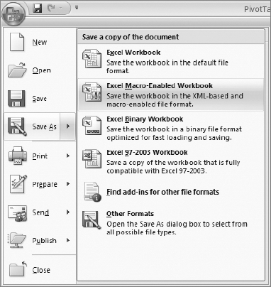
Figure 6-10. Saving the file as macro-enabled

Unfortunately, if we rerun the MakePivotTable macro again, we'll get an error, as shown in Figure 6-11.

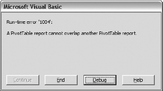
Figure 6-11. Running MakePivotTable a second time generates an error.

---

Note The runtime error 1004 shown in Figure 6-11 was generated in Windows XP. Windows Vista users will still see runtime error 1004, but its description will read "Application-defined or object-defined error."

---

We can't drop another PivotTable on top of an existing PivotTable. Let's make a few changes to our code to allow us to create our PivotTables dynamically based upon data that is?currently being viewed by the user.

There are two issues that stand out in our existing code:

• We have to add a new worksheet for an additional PivotTable for the data because we can't use the existing sheet (or we have to find a new location on the existing worksheet).
• What if the source data range expands (or shrinks) the next time we get this data?

In the VBE, add a new subroutine and name it MakeDynamicPivotTable. Copy the code from the MakePivotTable procedure, and then make the following modifications. Add the following variable declarations at the top of the MakeDynamicPivotTable procedure:

Dim ws As Worksheet
Dim rngRangeToPivot As Range
Dim sPivotLoc As String

The first variable, ws, will be used to store the new worksheet that we'll be adding. The next variable, rngRangeToPivot, will get the data source range for us regardless of number of rows. The last variable, sPivotLoc, will hold a string value denoting the range to place the new PivotTable.

The first thing we'll do is get the location of the data range that we'll be putting into our PivotTable. We'll do this first because once we add a new sheet, the data viewed by the user will no longer be active.

Add the following line of code to assign the current data region (the region where the cursor is currently placed):

Set rngRangeToPivot = ActiveCell.CurrentRegion

The ActiveCell.Current region property will retrieve the range of the contiguous set of cells surrounding the cursor location.

Now let's add a new worksheet and define the PivotTable location on the new worksheet:

Set ws = Sheets.Add
sPivotLoc = ws.Name & "!R3C1"

We're adding a new worksheet and assigning that worksheet to the ws variable. Then we're looking at that worksheet to determine its name and concatenating it to the cell location where the PivotTable will be place on the new worksheet. We're using Excel's default location of row 3/column 1, but you can place the PivotTable anywhere you like on your worksheet.

Finally, add the two commands shown in Listing 6-2 to make the PivotCaches.Create method and the PivotCache.CreatePivotTable table commands act on our new dynamic variables.

Compare this to the original version of these lines of code in Listing 6-3.

In the original code, the macro recorder set SourceData:="Sheet1!R1C1:R43C6". We changed that to refer to the rngRangeToPivot variable, SourceData=rngRangeToPivot. Regardless of how many rows are in the data range, the data source for our PivotTable will reflect the correct data.

The next line to compare is our call to the PivotCache object's CreatePivotTable method. The original code set the TableDestination to a location in a hard-coded reference to a worksheet: CreatePivotTable TableDestination:="Sheet4!R3C1". We replaced that with a call to our dynamic variable sPivotLoc, which refers to the name of the new worksheet we added, whatever that might be: CreatePivotTable TableDestination:=sPivotLoc.

The last difference is that the original code selects the hard-coded worksheet, Sheets("Sheet4").Select, while our new dynamic code simply refers to the ws variable and selects the worksheet it contains using the Worksheet object's Select method, ws.Select.

Listing 6-4 shows the completed MakeDynamicPivotTable subroutine.

Refreshing Data in an Existing PivotTable Report

How do we handle keeping our data fresh in a PivotTable? When rows are modified, added, or deleted, how do we pass that on to our PivotTable reports?

If our data had come from an external source like an Access or SQL Server database, refreshing the data would be as simple as running the following command with the PivotTable activated:

ActiveSheet.PivotTables("PivotTable1").PivotCache.Refresh

How do we handle updating our PivotTable data when the data does not sit in a DBMS? If the data on Sheet1 in our example is modified, how do we refresh the PivotTable?

When we created our macro to build the PivotTable, we assigned a dedicated range of data to the PivotTable using the ActiveCell.CurrentRegion property. The Refresh command cannot recalculate the CurrentRegion property we used because it knows nothing about it. So when we apply the Refresh command, whether through Excel's UI or via VBA code, it only refreshes the data range we initially supplied. Any values that have changed within that range (or any deleted rows) would be updated, but any additions to the data would not be applied to the PivotTable.

To update the PivotTable report we created, we will write a subroutine that determines the original data range of the PivotTable and uses that to recalculate the current data range. It will then apply that data range to the PivotTable's SourceData property, and then refresh the PivotTable.

In the VBE, create a new subroutine and name it RefreshPivotTableFromWorksheet. Add the following code:

Sub RefreshPivotTableFromWorksheet()
Dim sData As String
Dim iWhere As Integer
Dim rngData As Range

  sData = ActiveSheet.PivotTables("PivotTable1").SourceData
  iWhere = InStr(1, sData, "!")
  sData = Left(sData, iWhere)

  Set rngData =
    ActiveWorkbook.Sheets(Left(sData, iWhere - 1)).Cells(1, 1).CurrentRegion

  ActiveSheet.PivotTables("PivotTable1").SourceData =
                                          sData & rngData.Address(, , xlR1C1)
End Sub

Let's take a look at what this code is doing. We have three variables declared. sData will hold the value of the current range for the PivotTable's source data. We want to find the bang character (!) so we can retrieve the name of the worksheet the data came from. We'll store that in the iWhere variable. And finally, we have a variable of type Range, rngData, that will be assigned the CurrentRegion of cell A1 on the data worksheet. With this information, we have the tools to refresh our pivot data any time detail data is added on the data worksheet.

The first step is to get the current data source for the PivotTable:

sData = ActiveSheet.PivotTables("PivotTable1").SourceData

Next we'll find the ! character:

iWhere = InStr(1, sData, "!")

Now we want the worksheet name including the !:

sData = Left(sData, iWhere)

We modify sData because we only needed it to determine the worksheet name. The original data source range is going to be replaced, so we discard it at this time.

Now we'll assign the CurrentRegion property of cell A1 of the worksheet stored in sData to the rngData variable:

Set rngData =
    ActiveWorkbook.Sheets(Left(sData, iWhere - 1)).Cells(1, 1).CurrentRegion

Once we have the CurrentRegion, we can replace the current SourceData value of the PivotTable object with it:

ActiveSheet.PivotTables("PivotTable1").SourceData =
                                        sData & rngData.Address(, , xlR1C1)

We're passing in the xlR1C1 enum for the ReferenceStyle argument. This is the string format the SourceData property is looking for.

Now that we've set the SourceData for the PivotTable to the new CurrentRegion of the data worksheet, all that's left to do is call the Refresh command:

ActiveSheet.PivotTables("PivotTable1").PivotCache.Refresh

Let's give it a test. On Sheet1, add the following data to the grid for the city of Rochester, NY, as shown in Figure 6-12.

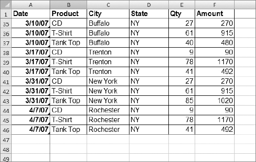
Figure 6-12. New rows added to PivotTable source data

Open Sheet4 (or the sheet your PivotTable is on, if different). Click any cell inside the –PivotTable. When the PivotTable is selected, a couple of new ribbons are displayed, as shown in Figure 6-13.

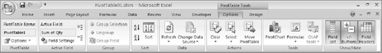
Figure 6-13. The PivotTable Tools ribbon (Options ribbon shown)

On the PivotTable Tools ribbon, select Options Data Refresh. Click OK on the Windows Vista security warning. Nothing happens—the Rochester data does not display.

On the Developer ribbon, run the RefreshPivotTableFromWorksheet subroutine. Now the new city appears in the data summary, as shown in Figure 6-14.

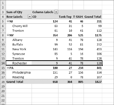
Figure 6-14. Rochester data displayed after RefreshPivotTableFromWorksheet is run

Applying Formatting to a PivotTable Report

You will probably find that some of the default formatting Excel applies to your PivotTable reports needs some modification—things such as the general number format, the table formatting without lines, the default naming of calculated fields to "Sum of field name," and its handling of null or blank entries.

In the Download section for this book on the Apress web site, find the file named PivotTable02_Formatting.xlsm, and open it.

Blank Data Records

To see the effect of blank records on a PivotTable report, let's make Sheet1 active and remove the data for Reading, PA's tank top sales. The Quantity and Sales Total values are 0, but we want to make them blank as though no data were added (as shown in Figure 6-15).

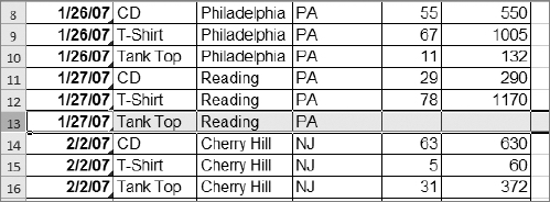
Figure 6-15. Blank data for Reading, PA tank top sales

1. Activate the worksheet containing the PivotTable report.
2. Refresh the data (either through the UI or the RefreshPivotTableFromWorksheet procedure). Figure 6-16 shows Excel 2007's default behavior when we have blank values in a PivotTable.

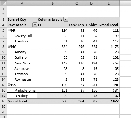
Figure 6-16. Blank values display as blank on PivotTable report

1. Drag the Sum of Qty label back up to the field selection list in the PivotTable Field List.

There is a little quirk that exists in the UI that you might encounter when coding PivotTables that bears a quick mention here. When Excel finds blank or null data in a range of data used in a PivotTable, and that field is used in the summary section, it defaults the summary field to "Count of field name" even though "Sum of field name" may be a more appropriate selection.

1. Drag the Qty field back down to the Values list.

Figure 6-17 shows Excel displaying "Count of field name" when we want to sum.

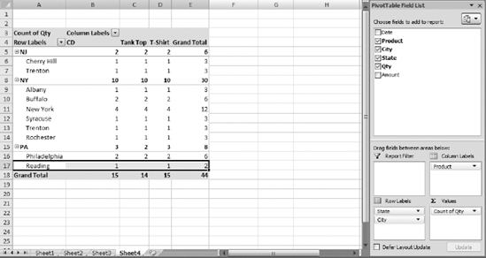
Figure 6-17. Count of Qty is the default due to the blank data record.

1. To prevent blank data from displaying, we can use the NullString property of the PivotTable object. In the VBE, add the following subroutine to the project:
   
   Sub ZeroForBlanks()
    ActiveSheet.PivotTables("PivotTable1").NullString = "0"
End Sub
   
   
2. From the Macros dialog box, run the subroutine. Figure 6-18 shows the result of running the ZeroForBlanks macro.
3. To fix Excel's inaccurate guess that we wanted to count the number of Qty records in the summary section of our PivotTable, we can use the Function property of the PivotField object. Add the following subprocedure to the standard code module:
   
   Sub ChangeSummaryFunction()
    With ActiveSheet.PivotTables("PivotTable1").PivotFields("Count of Qty")
        .Caption = "Sum of Qty"
        .Function = xlSum
    End With
End Sub

Once this code runs, the PivotTable will look like it did in Figure 6-16.

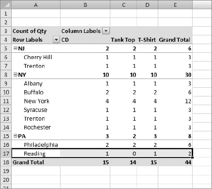
Figure 6-18. Zeros displayed instead of blanks

Table 6-4 lists the possible choices for the Function property.

Table 6-4. XlConsolidationFunction Enumeration

Name	Value	Description
xlAverage	−4106	Averages all numeric values
xlCount	−4112	Counts all cells including numeric, text, and errors; equal to the worksheet function =COUNTA()
xlCountNums	−4113	Counts numeric values only; equal to the worksheet function =COUNT()
xlMax	−4136	Shows the largest value
xlMin	−4139	Shows the smallest value
xlProduct	−4149	Multiplies all the cells together
xlStDev	−4155	Standard deviation based on a sample
xlStDevP	−4156	Standard deviation based on the whole population
xlSum	−4157	Returns the total of all numeric data
xlUnknown	1000	No subtotal function specified
xlVar	−4164	Variation based on a sample
xlVarP	−4165	Variation based on the whole population

Changing the Number Format

The default number format in a new PivotTable is Excel's general number format. Most of us like to see commas or currency symbols, which make the data more readable. To change the number format, you use the PivotField.NumberFormat property. The NumberFormat property sets or returns the string value that represents the format code for the numeric value. The format code is the same string value given by the Format Codes option in the Format Cells dialog box shown in Figure 6-19.

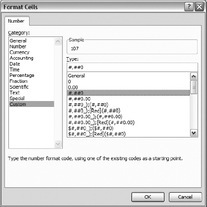
Figure 6-19. The Format Cells dialog box

Add the following routine to a standard module:

Sub FormatNumbersComma()
    With ActiveSheet.PivotTables("PivotTable1").PivotFields("Sum of Qty")
        .NumberFormat = "#,##0"
    End With
End Sub

Run the FormatNumbersComma subroutine from the Macros dialog box. The result should look like Figure 6-20.

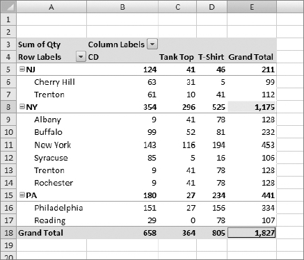
Figure 6-20. Grand Total rows with commas added

Changing Field Names

By default, Excel uses the name "Sum of field name" or "Count of field name" when you add summary value fields to a PivotTable. You can change the names to something with more visual appeal using VBA code.

Add the Amount field to the Values list in the PivotTable Field List. Change the Count value to Sum in the Value Field Settings dialog box (as shown in Figure 6-21) by clicking the Amount field in the Values list and choosing Value Field Settings from the right-click shortcut menu. Figure 6-22 shows the result of changing the field names.

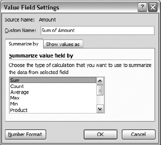
Figure 6-21. Value Field Settings dialog box

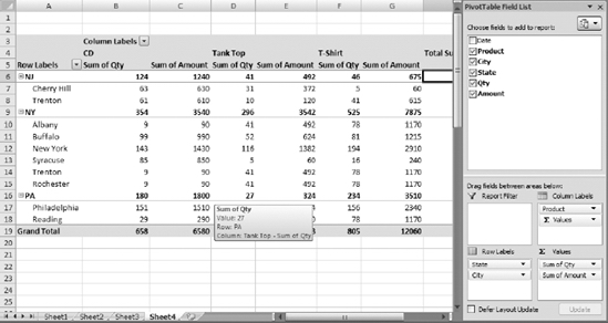
Figure 6-22. PivotTable showing Sum of Qty and Sum of Amount fields

Use the PivotField.Caption property to change the captions to something more easily readable.

Add the following subroutine to a standard code module:

Sub ChangeColHeading()
    ActiveSheet.PivotTables("PivotTable1").PivotFields("Sum of Qty").Caption =
        "Item Qty"
    ActiveSheet.PivotTables("PivotTable1").PivotFields("Sum of Amount").Caption =
        "Item Amount"
End Sub

Run the code from the Macros dialog box. The result should look like Figure 6-23.

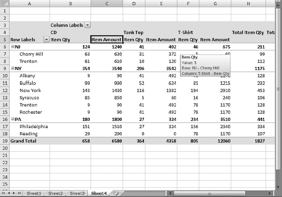
Figure 6-23. Summary field headings modified

Adding Formatting to a PivotTable Report

The default PivotTable report Excel generates looks okay, but Excel 2007 does provide us with 75 different formatting options. To change the look of a PivotTable report using VBA code, use the PivotTable object's TableStyle2 property. This property is named TableStyle2 because there is already a TableStyle property (but it's not a member of the PivotTable object's properties—go figure).

Add a new subroutine to a standard code module and add the following code:

Sub ApplyTableStyle()
    ActiveSheet.PivotTables("PivotTable1").TableStyle2 = "PivotStyleLight1"
    'ActiveSheet.PivotTables("PivotTable1").TableStyle2 = "PivotStyleLight22"
    'ActiveSheet.PivotTables("PivotTable1").TableStyle2 = "PivotStyleMedium23"
End Sub

Before we run this code, let's remove the Item Qty field from the Values list in the PivotTable Field List to make the PivotTable smaller and the formatting easier to see.

Run the code from the Macros dialog box to apply the PivotStyleLight1 formatting to the PivotTable, as shown in Figure 6-24.

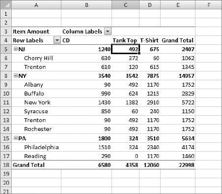
Figure 6-24. PivotStyleLight1 formatting applied

Comment out the first line of code in the ApplyTableStyle procedure and uncomment the second line. Run the subroutine from the Macros dialog box to apply PivotStyleLight22 format–ting, as shown in Figure 6-25.

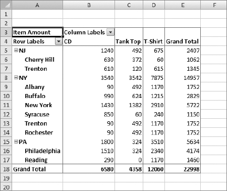
Figure 6-25. PivotStyleLight22 formatting applied

Comment out the second line of code in the ApplyTableStyle procedure and uncomment the third line. Run the subroutine from the Macros dialog box to apply PivotStyleMedium23 formatting, as shown in Figure 6-26.

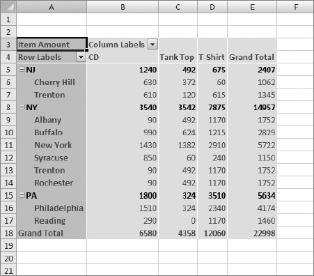
Figure 6-26. PivotStyleMedium23 formatting applied

Summary

PivotTables in Excel 2007 provide users with a very easy-to-use interface with which they can analyze and summarize large amounts of data. In this chapter, we took a look at code generated by Excel's Macro Recorder to get a feel for the PivotTable and PivotCache objects' properties and methods. We then saw how we could modify that code to make it more flexible and dynamic.

Excel 2007 PivotTable reports are not linked to their data, but use the PivotCache object to store a pointer to the data. When the data on a worksheet changes, the PivotTable does not automatically update with those changes, especially if new data is appended. We created a method to let the user refresh the PivotTable if the worksheet data on which it was based was appended to.

Finally, we looked at some of the formatting options available to us using VBA code. We were able to fix some of Excel 2007's default formatting behaviors, such as its use of the general number format, generic summary field names, and its handling of blank rows. We also saw how applying styles can dress up a PivotTable report.