
Now that you (hopefully) have a rudimentary understanding of the Internet and web technologies that power it, let’s move forward to a skill that every PM needs in their toolset: SQL. SQL (pronounced “see-quill” or “S-Q-L” depending on preference) stands for Structured Query Language, and is used for creating, transforming, and manipulating data in a relational database. A relational database is an information system that exists to structure data in rows and columns for easy read and write alterations. For example, let’s take a look at an example SQL database table for vehicle data:
ID | Make | Model | Color |
|---|---|---|---|
1 | BMW | 328i | White |
2 | Mercedes-Benz | CLA 250 | Black |
3 | Acura | TSX | Blue |
4 | Porsche | 911 | Red |
As you can see, each column of data is indicated with a header label, and all fields are represented in rows underneath. If you’re familiar with cells in Excel, the concept of how and why a table is structured in this way will become immediately clear as we walk through this chapter. At a basic level, SQL enables a developer or analyst to build new databases and tables in a quick, repeatable manner and add data to them easily. On the flip side, SQL can allow you as a product manager to pull data directly from the database without chewing up engineering cycles. PMs who can master the art of querying tables can save their development team significant time on data pull requests, and enable themselves to chop the data up in creative ways to identify patterns at will. Whenever an application requires back-and-forth interaction with a set of data (e.g., posts on Facebook, movie titles on IMDb, movies on Netflix, etc.), you can almost guarantee that a database is involved in some form or fashion. Although different implementations of relational databases exist on the market (MySQL, Microsoft SQL Server, PostgreSQL, etc.), the underlying syntax is common (if not identical) between all the products. We’ll be using mostly mySQL syntax in this chapter since it is one of the most popular and widely used offerings on the market. In this section, we’ll cover basic SQL statements used for data handling, walk through the process of joining sets of data together, and touch on advanced topics in a broad strokes view. Don’t worry, it’s easier than it sounds.
And with that, let’s jump right into writing SQL statements!
Definition
A “query” is a statement issued to a database to return information. In the scope of a SQL database, a query encompasses anything typed into a terminal or GUI (graphical user interface) that is a direct command for data retrieval.
CREATE, DELETE, and SHOW database
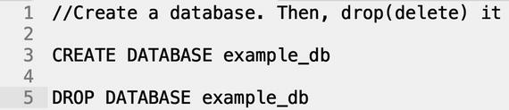
Before we set out on a journey to harness the power of raw data and become SQL wizards, we need to create a database to store the information. A database is simply a collection of tables, and houses data for future use. For example, a car dealership database (car_db) can contain tables such as inventory_table (tracking available cars), orders_table (records all historical purchases), HR_table (employee information), and so on. As you’ll soon notice as you step through this chapter, SQL is an intuitive language because it uses simple terms to define the commands. In this scenario, the statement to create a new database is CREATE DATABASE, and the action to delete the newly created database is DROP DATABASE. The same structure can be used to add and delete tables inside the databases as well (CREATE TABLE [name] & DROP TABLE [name]). Once the database is created and defined, we can populate it with tables and send commands for data retrieval.
Query:
To confirm that a database has indeed been created, you can use the SHOW DATABASES command. If a list emerges with the previously named database, then everything is working as intended. If a blank list is thrown back, then you may have to revisit your creation step.
Query:

SELECT statements
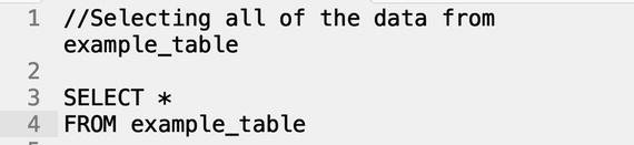
A SELECT statement is the most common SQL command used to retrieve data: it tells the database what data you want fetched. If we wanted to write a query that will return all of the data in our vehicle table (named example_table), we would issue the following.
Query:
Result:
ID | Make | Model | Color |
|---|---|---|---|
1 | BMW | 328i | White |
2 | Mercedes-Benz | CLA 250 | Black |
3 | Acura | TSX | Blue |
4 | Porsche | 911 | Red |
Let’s break this command down.
- 1. The two forward slashes (//) denotes a comment to explain the query. It reinforces the goal of the query that we’re executing, and only exists to help you, the reader, understand what we’re doing. Also, ignore the line numbers. I’m using Sublime Text as my IDE (integrated development environment), and it automatically numbers the lines on the fly. They have no relation to the query being issued.
- 2. The SELECT defines the main command we want the database to interpret.
- 3. The asterisk (*) is a catch-all for everything in that table. It essentially translates to EVERYTHING in simple terms.
- 4. The FROM describes which table we want to pull data from (in this case, example_table).
- 5. Formally issue the command, and all of the rows and columns are displayed.
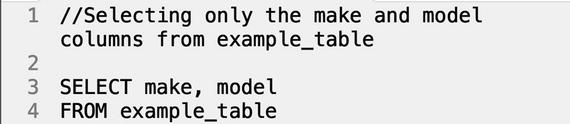
Great! But what if you want to return only the make and model of the car? Let’s change up the original statement to fit our new requirements.
Query:
Result:
Make | Model |
|---|---|
BMW | 328i |
Mercedes-Benz | CLA 250 |
Acura | TSX |
Porsche | 911 |
In this case, we’re asking the database to return ONLY the make and model columns instead of the entire table. If the user wants to include the “color” column, all they have to do is add in “color” to the SELECT query after “model”.
Simple so far, right? Let’s keep pushing forward.
SELECT statements with conditions
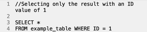
At this stage, you may be wondering: “What about the rows? How do we prevent the entire data dump from being surfaced every time we run the command?”
Good question. Cutting and filtering the data in a useful fashion requires operating on both dimensions, so we use the WHERE operator to specify the constraints.
Query:
Result:
ID | Make | Model | Color |
|---|---|---|---|
1 | BMW | 328i | White |
In addition to specifying values that already exist in the table, the WHERE operator can also be used for comparisons and logic operations (<, >, =, LIKE, and NOT). Imagine a table listing cost and locale of food items in a region, as shown below, and you were a PM tasked with completing a competitor analysis.
Item Number | Name | Price | Zip Code |
|---|---|---|---|
132452123 | Sunflower Seeds | $3.45 | 96035 |
43656455 | Apple Pies | $12.44 | 39503 |
59049304 | Nutella | $5.44 | 85033 |
If we were to kick off an assessment and wished to trim the data based on price and zip code, we could couple the WHERE operator with the AND operator to chain commands together, as shown in the following sample query.
Query:

Result:
Item Number | Name |
|---|---|
59049304 | Nutella |
SQL operator breakdown
AND: Both statements must be true for data to be returned.
SELECT *
FROM NFL_teams
WHERE name = 'Tom Brady' AND team = 'New England Patriots'
OR: Either the first condition or the second condition must be true for the data to be returned.
SELECT *
FROM product_info
WHERE price > 20 OR discount_status = 'clearance'
NOT: All data is returned except for condition specified by NOT. NOT is exclusionary, and exists to return the opposite of the specified state.
SELECT *
FROM universities
WHERE name IS NOT IN ('Cornell', 'Harvard')
The commands we’ve been issuing are on miniscule data sets with less than five rows, but using the WHERE clause coupled with complex operator combinations on tables with hundreds of thousands of rows (possibly millions) can lead to insights that influence product decisions and break the holistic data view into digestible chunks.
UPDATE table with new data
So far, we’ve been exercising our ability to read data from a database, but for data freshness and overall practicality, we need the power to update and add data. Using UPDATE, we can identify a row, set a new value, and finalize the change. Our example_table with vehicle data incorrectly uses a discontinued model name for Acura, so let’s use UPDATE to correct this mistake.
Query:
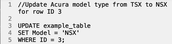
Table contents after UPDATE is run:
ID | Make | Model | Color |
|---|---|---|---|
1 | BMW | 328i | White |
2 | Mercedes-Benz | CLA 250 | Black |
3 | Acura | NSX | Blue |
4 | Porsche | 911 | Red |
DELETE table rows
Conversely, instead of updating data from the table, the DELETE command removes rows completely. DELETE can be used with conditions, or as a blanket command using the structure DELETE [tablename] to clear all of the contents of a table, so be sure to exercise caution to avoid erasing all of your data with a mistake query!
Query:
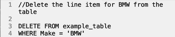
Result:
ID | Make | Model | Color |
|---|---|---|---|
2 | Mercedes-Benz | CLA 250 | Black |
3 | Acura | NSX | Blue |
4 | Porsche | 911 | Red |
ORDER BY
The ORDER BY command
is positioned well to sort data and trim the rows returned to a manageable size. ORDER BY takes column names as a parameter, and arranges them in ascending order by default, with an option to convert to descending by appending DESC to the end of the query. If the table you’re dealing with contains thousands of rows and you want a subsection of the full view from a top down perspective, use the LIMIT command to restrict the number of rows that are returned.
Query:
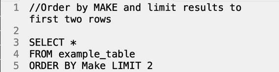
Result:
ID | Make | Model | Color |
|---|---|---|---|
3 | Acura | NSX | Blue |
2 | Mercedez-Benz | CLA 250 | Black |
JOINS
The last command we’ll cover is the concept of a table join in SQL. Joins allow data from multiple tables to be combined using similar columns that exist in both tables. In total, four common joins are typically used to merge table contents together.
Left Join: all rows from the left table are retrieved, along with matching rows from the right table.
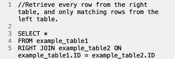
Right Join: all rows from the right table are retrieved, along with matching rows from the left table.
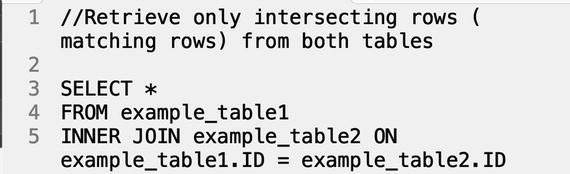
Innner Join: only matching rows belonging to both tables are retrieved.
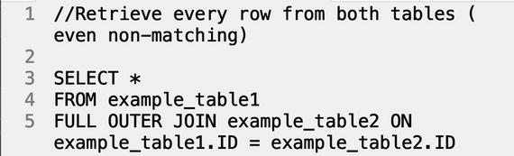
Outer Join: retrieves all rows from both tables.
To better illustrate this point, we’ll walk through each join type step-by-step using the following example tables.
Table 1.
example_table1
ID | First Name |
|---|---|
1 | Grant |
2 | Rob |
3 | Femi |
Table 2.
example_table2
ID | Last Name |
|---|---|
1 | Tall |
2 | Lee |
4 | Haque |
5 | Oje |
LEFT JOIN (also called LEFT OUTER JOIN)
A left join
will return all values in the left table (the table defined first in the query) and join against all of the matching values on the right table (table listed after the LEFT JOIN indicator). Companies don’t hold all of their data and information in one single database. Instead, grasping the concept of table joins will help you identify common fields and stitch the data together across tables. Aside from using the JOIN operator, we also need to use ON to establish which column we want to use to join the data. Both tables must have one column with a linking key for a join to be successful. A primary key is a distinct ID (e.g. integer) used to assign each row in a table a unique identifier. The foreign key is the mapping value; in essence, it is the same value that sits in another table that can be used to join the two together. The primary / foreign key paradigm can be hard to understand at first, so I recommend follow up research if the queries below are difficult to digest.
Query:
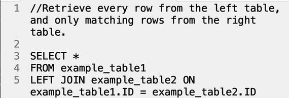
Result:
ID | First Name | Last Name |
|---|---|---|
1 | Grant | Tall |
2 | Rob | Lee |
3 | Femi | null |
Note
the “null” value that surfaces when we return this set of data indicates no value in the right table that matches the ID of 3.
RIGHT JOIN (also called RIGHT OUTER JOIN)
A right join
will return all values in the right table (the trailing table in the JOIN command) and join against all of the matching values on the left table. Notice that the positioning of the tables in the query doesn’t change, since first placement signifies left table and second placement is associated with the right table.
Query:
Result:
ID | First Name | Last Name |
|---|---|---|
1 | Grant | Tall |
2 | Rob | Lee |
4 | null | Haque |
5 | null | Oje |
INNER JOIN
An inner join
will return only the values that match in BOTH tables. Depending on what you specify as the join criteria, the results returned can vary between queries.
Query:
Result:
ID | First Name | Last Name |
|---|---|---|
1 | Grant | Tall |
2 | Rob | Lee |
OUTER JOIN (also called FULL OUTER JOIN)
An outer join
will return every row in both tables, even non-matching pairs. If the rows happen to match, then they will only populate one row. For example, in the resulting table below, we don’t have one unique row for ID 1, Grant and another unique row for ID 1, Tall. Common records are merged together, and mismatched rows use the null designation.
Query:
Result:
ID | First Name | Last Name |
|---|---|---|
1 | Grant | Tall |
2 | Rob | Lee |
3 | Femi | null |
4 | null | Haque |
5 | null | Oje |
Note
MySQL doesn’t support FULL OUTER JOIN at the time of this publication. To replicate this function, you will need to use the UNION operator instead and thread together a left and right join.
Advanced topics
We’ve covered a lot in this chapter, but there’s still a lot more to know about SQL and relational databases. If you’re ready and willing to go deeper down this rabbit hole, I’ve brushed over some advanced topics below. Note that I’ve left out details and simplified a few of the concepts listed, but you will sharpen your understanding as you do more independent research. The goal is to get you curious enough to learn on your own and move closer to mastery at your own pace.
Indexing:
Dealing with massive tables with millions of rows can be difficult from a data processing standpoint because the queries will take minutes (or even hours) depending on complexity and available processing power. To speed up the data fetch, you can create indexes against your database, and avoid having to rerun the entire query each time. To frame this in a simpler fashion, think about searching for a word in the dictionary. You can spend time flipping through the pages, one by one, until you finally arrive on the correct definition, or you can skip to the index in the back of the book and find the exact page without having to perform a manual search operation each time. A database table index allows you to do the same, and save processing time by avoiding unnecessary database operations.
Normalization:
Falling in the domain of database design, normalization splits the data into logical tables so redundant work can be avoided. For example, imagine a 1,000,000 row table with name, address, and magazine subscription name. If John Doe has 12 entries in the table because he’s moved a bunch of times, then we’ll need to update his address in 12 different places the next time he moves (one time per row). Instead of this long and arduous process, we can split the main table into two tables: one for name and magazine subscription name, one for address and link the two with a set of primary and foreign keys. This way, if John’s address needs to be changed, it only has to be updated in the address table one time.
Sharding:
An advanced technique that splits the database into smaller chunks called “shards” to push across distributed servers. Sharding improves processing performance and enables segmentation of data based on permissions rules the developer creates (e.g., US users vs. EU users). At a local level, instead of running queries on your individual laptop or desktop, you can shard the data and process information across clusters in the cloud for faster results.
NoSQL:
A new wave of databases that break free of the traditional relational model. noSQL databases are often used for big data sets, and can offer advantages over relational databases depending on use case.
ACID: Atomicity, Consistency, Isolation, and Durability. ACID comes into play when dealing with concurrent transactions in databases (checking out items, paying for goods/services) and guarantees the security, validity, and quality of the data in the event of an error or failure when transactions are executed.
Data sanitization / database security:
Changes are made to a database based on the SQL queries that are issued to it, so we must be careful about protecting the back end from any malicious queries. Allowing a user to input data into an application that doesn’t go through a proper sanitization process could leave your data vulnerable. A variety of front-end (input validation) and back-end techniques (query monitoring) can be leveraged to prevent SQL injection from damaging your products or applications.
UML: Unified Modeling Lanugage (UML)
is a standardized method to visualize all of the design components of a system. UML diagrams are used to create schemas that map the tables to one another and describe the relationships between each entity (one to one, one to many, etc.). Before any development work is done, a well-crafted UML diagram can be a quick look into whether the system makes sense and data is appropriately bucketed into the right locations.
Informative…but why is this useful to me as a PM?
Whether you’re joining a newly launched startup or a mature technical firm, both value two key variables: time and money. When you’re engaged in an arms race of innovation against other companies, time is everything, and distracting engineering resources away from building hard features can be costly. A PM who can be a data wrangler and build their own view of the data without a helping hand can be a welcome relief to the engineers, and it can be a quick and easy way to get respect within the team. SQL is a language that can be learned in a short period of time at an intermediate level, so dedicating the effort to practice the commands and dig into the advanced topics will only be advantageous for you in the long run, and a data-driven PM is only made more effective with SQL expertise.
Note
Practicing with or running SQL queries should generally be done in a non-production environment. Running queries in a production environment risks exposure of sensitive information as well as affecting mission-critical operations. Generally, there is no good reason why you would need to query a production database rather than a copied version of that data on a completely separate non-production system. Following best practices ensures that you aren’t the person making the news for deleting all of your company’s data, or for having your laptop filled with sensitive data stored on it stolen from your car (encrypted or not).