
5 Scheduling
The term “schedule” commonly brings to mind the graphical representation of the project activities, including the duration of each activity, the interrelationships among activities, the dates of calculated or imposed milestones, and possibly the completion date of the project. The schedule can be represented graphically in different formats: Gantt charts, milestone charts, or schedule logic networks. These graphical presentations should be based on quantitative data derived from calculations.
Scheduling is not merely the process of assigning calendar dates to the completion of activities of the project, however. It also is the art and science of developing a predicted delivery or completion date for the project by way of developing a logical sequence structure for the project’s activities. The foundation of the scheduling process is the logical sequence of the elements of the schedule network, and this sequence serves as the basis for planning, resource allocation, and resource leveling.
The data provided as part of the scheduling process support management decision-making about a project’s time, cost, and risk management issues. Although calculations can be performed using the sequence logic depicted in a tabular manner, sometimes using the visual depiction of the network diagram is more convenient for conducting schedule computations. Additionally, some schedulers include many of the results of the scheduling calculations directly on the network diagram.
During the early planning stages, a total overall estimate of project duration can be obtained using any one of the estimating models described in the earlier chapters. However, as more details of the project become available, a more definitive, more logical, and more accurate depiction of the project’s duration will become necessary.
A detailed set of WBS and RBS, and the resultant time estimate for each project element, are prerequisites to developing a project schedule (see Figure 5-1). Whereas estimating the cost of higher-level WBS elements is achieved by rolling up the costs of corresponding lower-level elements, estimating the duration of the higher-level WBS elements, and the project, is dependent upon the execution sequence of the lowest WBS elements, as indicated in the logic network. As the details of the project become more accurate, the project’s duration and delivery date can be calculated using the network logic diagram (see Figures 5-2 and 5-3).
The logic network is constructed in the context of the interdependency of activities as indicated by work-related constraints. The network diagram will show the sequencing relationship among the project’s activities. The estimate of the project’s duration will be obtained by calculating the longest chain in the network in light of the sequence of activities and using the estimated activity durations. This chain also represents the shortest duration of the project, given the current logic and the optimum duration of individual elements and activities.
The calendar start date is not required for developing the logic diagram, calculating the floats, or identifying the critical path. However, to assign calendar dates for the start and finish of activities, and the project as a whole, a calendar start date is necessary.
Figure 5-1
Estimating


Figure 5-3 Scheduling

TWO BASIC NETWORKING TECHNIQUES
There are two basic techniques for developing the schedule network and displaying the relationships among the activities of the network (see Figure 5-4): the Critical Path Method (CPM), also known as the Activity on Arrow Technique (AOA) or the Arrow Diagramming Method (ADM); and the Program Evaluation and Review Technique (PERT), also called the Activity on Node Technique or the Precedence Diagramming Method. These sets of names and their associated acronyms highlight the different features of these techniques.
The CPM, or AOA, technique identifies each activity with two numbers, one signifying the start point and the other signifying the end point (see Figure 5-5). To depict activity relationships fully, additional relationships among activities must be signified by arrows between activities. These additional relationships are shown using elements that are called dummy activities. Dummy activities are similar to normal activities in notation, except that they are not real activities because there are no resources attached to them, and their duration of execution is zero.
Figure 5-4
Schedule Network Diagramming Methods

To illustrate, Figure 5-5 shows that Activity F has two predecessors, Activities A and D. To maintain identity and correct linkages, a dummy activity is shown between nodes 2 and 5, which requires no resources and does not consume time. As noted, the AOA notation for network activities contains the relationship information, which makes it easy to store and transfer network information. Additionally, the logic network can be drawn simply from the list of activities.
Figure 5-5
Arrow Diagramming Method

The PERT technique, otherwise known as the AON, identifies each activity with one number (see Figure 5-6). On the other hand, another instrument called the Precedence Table would be needed to specify the necessary activity relationships (see Figure 5-7). The other difference between the AOA and AON techniques is that in an AOA network the relationship between two successive activities is usually in the simple finish to start (FS) mode, whereas in a AON network the activity relationships can be signaled by three other relationship notations, namely, start-start (SS), start-finish (SF), and finish-finish (FF).
Figure 5-6
Precedence Diagramming Method

Figure 5-7
Precedence Table
Notwithstanding the differences, these two techniques have several similarities. Both use forward pass and backward pass to identify the critical path and the amount of floats for noncritical activities. The resulting critical paths will have the same duration and the same floats for the non-critical activities. Further, even though the PERT technique was the first technique to use statistical analysis of the project duration and its associated probability distributions, a CPM network also can benefit from the same set of calculations.
Both of these techniques were used with equal frequency until the mid-eighties. Since then, due to the influence of software tools and other historical issues, the AON technique has gained much more popularity and much wider use. Accordingly, we will use this technique in most of our examples and illustrations.
COMMON CALCULATIONS
Two sets of calculations, forward pass and backward pass, are fundamental to the process of calculating the duration of the project (see Figure 5-8). During the forward pass, go forward from left to right, adding the duration of each activity to the duration of the chain of activities at that point. This set of calculations will take you from the start of the project to its completion in many separate activity chains. The forward pass will identify the shortest duration of project implementation, which is the longest chain within the project, known as the critical path.
Additional information can be obtained from the network data by conducting a backward pass. During the backward pass, go backward from right to left, subtracting the duration of each activity from the duration of the chain of activities at that point. This set of calculations will take you from the end of the project to its start point in all of the activity chains.
Figure 5-8
Schedule Network Diagramming Methods
When conducting the forward pass and the backward pass, one of two notations can be used for the addition and subtraction of durations and for the start and finish dates of activities. One is the traditional schema in which the starting point of an activity is 8 a.m. of the start day, and the end point of the activity is 5 p.m. of the finish day. For example, if a sequence of activities includes two activities of three and five days’ duration, respectively, the start and finish days of the first activity are 1 and 3, while the start and finish of the second activity occur at day 4 and day 8.
The second calculation schema has been introduced in the past 20 years and is used primarily in the IT industry. It uses 5 p.m. as the start point of one activity and the end point of another activity. Using this notation, the start–finish days of the activities in the example are 0–3 and 3–8.
Schedule calculations of a forward pass and a backward pass depend on good estimates for the durations of the activities and a realistic sequencing logic. The relationship among activities is represented by a precedence table in which the order of execution is highlighted. The precedence table is refined by using a relationship qualifier, which can be FS, FF, or SS.
Figure 5-9 shows the graphic depiction of these relationship qualifiers. Additional helpful information for a good schedule is the appropriate lead and lag times, which should be based on experiential data representing good practices. A lag signifies the number of units of time by which an activity, in an FS relationship, must delay its start after the preceding activity has been completed. Conversely, a lead signifies the number of time units by which a succeeding activity will start before the preceding activity is completed.
Forward pass involves calculating the project duration from project start to finish (left to right), which would help to determine the earliest time when an activity can start (ES) and the earliest time when it can finish (EF). The ES and EF of an activity are determined by adding the duration of an activity to the finish date of the activities preceding it.
Backward pass computation will use the project duration that was calculated as part of the forward pass as the starting point of the computations. Then, the latest time when an activity can start (LS) and the latest time when an activity can finish (LF) can be determined. The LS of an activity will be determined by subtracting the duration of an activity from the LS of its succeeding activity.
Figure 5-9
Activity Relationships

The significance of ES and EF are that the dates are the earliest dates that the activity in question can start and finish without affecting other activities. Likewise, LS and LF flag the latest date at which activities can start and finish without affecting other activities. By comparing the data from the forward pass and backward pass, namely the values for ES-EF-LS-LF, one can determine the float of an activity, also known as slack. The float can be determined either from LS-ES or LF-EF. (If these two computations result in different floats for the same activity, there is an error in the previous computations.)
The float of an activity is the amount of time that the activity can be delayed without affecting the start date or finish date of other activities. Low values of float, and a small number of activities that have float, will signal the extent to which the project is likely to require complex schedule management policies to remain on target. On the positive side, high amounts of float, and a large number of activities with float, in a network denote flexibility associated with managing the project schedule.
Some of the activities in the network diagram will have identical values of ES and LS, or EF and LF. In other words, these activities will have zero float. The string, or strings, of activities in the network that have zero float is called the critical path of the network (see Figure 5-10).
The critical path determines the total duration of the project, which is the longest chain of the network. It is possible that a project may have more than one critical path but the duration for all critical paths is equal. A delay in any of the activities on the critical path will delay the project completion by the same amount.
Figure 5-10
Critical Path

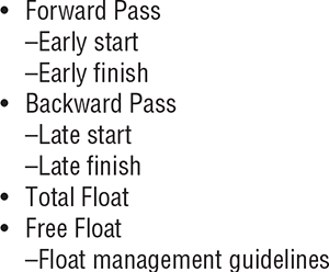
Figures 5-11 through 5-15 demonstrate the project network development and schedule calculations. Figure 5-11 shows the activity name, its ID, duration, and precedence list of a network. For simplicity, all the relationships are shown as finish to start (FS), which is the default in network development. Using the duration values and precedence relationships, a network schedule is developed (see Figure 5-12).
After the project network logic is defined with interdependencies, forward pass calculations will calculate the early start and early finish values, which can be added right on the network (see Figure 5-13). Figure 5-14 then shows the results of the backward pass. The key in these passes is that the forward pass is conducted by adding durations, whereas the backward pass is conducted by subtracting durations. Finally, a comparison of the early and late values will determine the amount of float (total float) for these activities.
Figure 5-11
Schedule Calculations (Activity List and Precedence List)

Figure 5-12
Schedule Calculations (Durations and Network Logic)

Figure 5-13
Schedule Calculations (Early Start, Early Finish)

Figure 5-14
Schedule Calculations (Late Start, Late Finish)

Figure 5-15
Schedule Calculations (Float)
There are two different categories of float: total float and free float. The amount of float that is calculated from the subtraction of, for example, LS-ES, will signify the total float of that activity. In most cases, the free float is the same as the total float. However, if the network contains a stand-alone chain of several activities, they would end up having the same amount of float.
To say that all of these activities can delay their start by the amount shown would be inaccurate. Rather, the float that is shown for these activities, which is the identical value, should be shared among these activities. In other words, in many ways these activities should be treated as though they were on the critical path, because if any one of them uses the float, that will disturb the start and finish dates of the other activities in that chain. Therefore, although the total float for these activities might be six, the free float for all of them is zero. The process by which the project manager will allocate all or portions of this float to any of the activities in this chain is called “float management.”
The example shown in Figure 5-14 uses the traditional schema for start and finish values. In traditional schema, the starting point of an activity is at 8 a.m. of the start day, and the end point of the activity is at 5 p.m. of the finish day. Accordingly, Element A, which has a duration of five days, has Day 1 as the earliest start day and Day 5 as the earliest finish day. Since Activity A precedes Activities B, C, F, and I, all these four activities will have the same earliest start date, i.e., Day 6.
Using the same logic, the ES and EF of all other activities are calculated. The EF calculation of Activity E, which is the last activity of the project, is particularly important. The earliest finish date of Activity E is 29, which implies that the project duration is 29 days.
Starting from Activity E and an EF value of 29 days as the basis, backward pass calculations are made (see Figure 5-13), which are shown in a separate box below each activity. The Activity E latest finish date will be same as the earliest finish date, as this is the final activity of the project. The latest start date of Activity E is derived by subtracting its duration from the project finish duration, which is 29 days; thus, the LS for Activity E is 25 days.
Since Activities B, D, H, and J are predecessors to Activity E, all will have the same latest finish date, i.e., Day 24. By subtracting its duration from 24, the LS for B, D, H, and J are calculated. Using the same logic, the LS and LF of all other activities are calculated.
After both forward pass and backward pass calculations are completed, the next step of schedule computations is to determine float for each activity. The float of an activity is calculated by subtracting the ES from the LS or the EF from the LF (see Figure 5-15). Float values shown in Figure 5-15 indicate the total float. For example, if Activity C is delayed by two days, then the ES for Activity D will change from nine to 11. However, the free float of an activity will not affect the ES of its succeeding activity.
To illustrate this concept, Activity B has 12 days of free float. By delaying it up to 12 days, the ES of Activity E will not change. Compared to Activity C, the delaying decision of Activity B will require less or no coordination with the project team.
An example of the distinction between free float and total can be found in Activities I and J. Both of them have a float of 14 days, with the implication that each one can be delayed by 14 days without affecting the project. Given that they are in a stand-alone string, they share the 14 days, and therefore the free float is zero. The project manager might choose to distribute the 14 days between these two activities, e.g., 5 and 9, or 14 and 0.
Finally, float calculations reveal the critical path of the project, which is A-F-G-H-E. All these activities have zero float, and delay in any of these activities will result in delay in the project.
SCHEDULE MANAGEMENT
Given that the same WBS is used for the formulation of the elemental cost and for the schedule network, the scope, cost, and schedule are closely integrated. Beyond that, all considerations of risk also can be incorporated into this integrated plan, during the planning phase as well as during the execution of the project. Naturally, any updates that are made to the project plans (and there should be regular and frequent updates) will be evaluated in the light of all of these integrated plans.
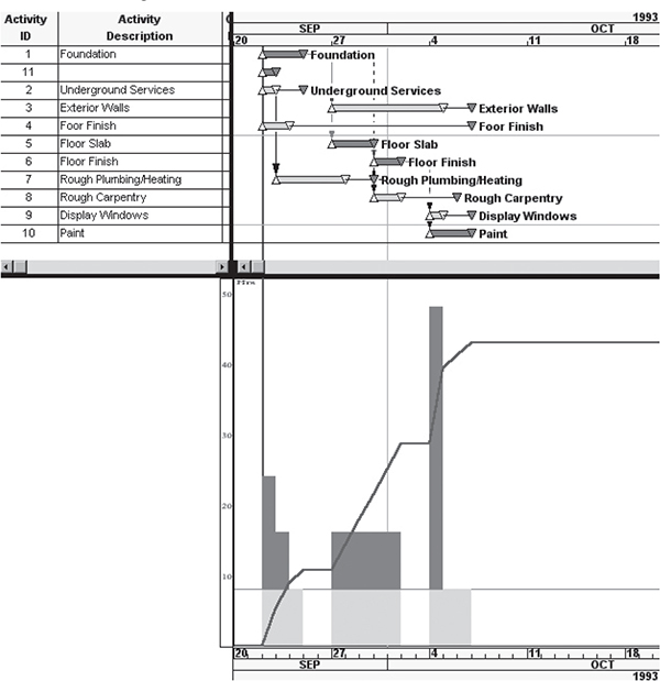
Resource usage over time is normally depicted in a vertical bar chart histogram and is commonly referred to as the resource histogram. With the resource requirements for each WBS element for each of the time periods of the project life cycle, and ultimately for the project, you can develop a resource histogram for each of the project’s resources (see Figure 5-16). The full suite of histograms will highlight the resource requirements for all of the resources spanning the full spectrum of the project life cycle.
Resource utilization and resource histograms must take the work calendar into consideration (see Figure 5-17). As discussed in traditional schema, the traditional work calendar starts at 8 a.m. and ends at 5 p.m., including a non-working hour for lunch break, which should be taken into account for resource calculations. Likewise, working days of the week, holidays, and seasonal adjustments, which will affect productivity, also should be considered in making resource calculations.
Figure 5-16
Sample Schedule with Resource Histogram

Figure 5-17
Work Calendar

A major level of planning sophistication can be achieved by developing a pristine integrated plan for the project, even before overlaying the client and environmental constraints. The pristine plan would be the optimum project plan, i.e., a plan that is unencumbered with milestone constraints and low resource availability, and therefore is poised to deliver the project in the utmost efficient and cost-effective manner. By definition, a pristine schedule will not have any resource overloads because it presumes that the project can have as many resources as it needs for the optimum delivery of the project results.
Then, in response to the inevitable changes in the project environment, the project schedule would be altered to meet client requirements in resources or milestones, with possible impact on project cost. This is indicated by a company-specific optimum curve, or at least by the generic optimum curve. If the project duration needs to be compressed below the optimum duration to comply with the client’s request for an early delivery date, then the resource histogram of the compressed schedule would provide an indication of the additional resources that might be necessary to effect the desired compression.
On the other hand, if there are resource limitations, you can conduct a leveling process on the network. The leveling process involves delaying activities of the project to reduce the overall resource demand for a particular resource (see Figures 5-18 and 5-19). Alternatively, if the project cannot be delayed, and if additional resources can be obtained, the histogram will help determine the amount of additional resources that would be needed.
During the project’s execution period, it is very likely that costs associated with most of the resources will change from the original estimated values, which will affect project cost and may prompt initiatives to schedule changes to maintain the original cost plan. The probability of such resource cost or schedule changes is higher for projects with longer durations.
Likewise, during project execution, it is very likely that a project will experience changes in schedule due to unexpected happenings and unanticipated activities. As a result, schedules will be subjected to enhancements and updates (see Figure 5-20).
While cost and schedule changes can be triggered by enhancements and updates in deliverable information, modified client objectives also can trigger a schedule adjustment. These objectives can initially affect cost, schedule, quality, or resource availability.
Figure 5-18
Resource Histogram with Overload
Administrative milestones often can result in durations for segments of the network that are shorter than anticipated by the current project baseline. This situation is sometimes called negative float. The remedy for a negative float situation is to implement some form of schedule compression.
At the other end of the spectrum, if the project demands more cash flow than the client can provide, then the remedy would be to expand the duration of the project in line with the client’s cash flow abilities (see Figure 5-20). Expanding a schedule also will add to the project’s total cost, however.
Figure 5-19
Resource Histogram Leveled

Figure 5-20
Schedule Adjustments during Maintenance Phase

Schedule compression often is triggered by new and more constrictive client requirements for the completion date. Sometimes, when the original schedule was expanded in response to a shortage of resources, then reverting back to a shorter schedule might be regarded as compression, although in reality it is not.
Schedule compression is almost always accompanied by an increase in project cost, unless, of course, if the current baseline is an expanded form of the pristine schedule. In addition to an increase in cost, there also might be an accompanying increase in delivery risk when the project is compressed.
Since only critical path activities can be considered for compression, they must be prioritized based on the cost penalty associated with their compression. This prioritization can be on the basis of cost, risk, resources, or simply ease of compressing a particular activity. Specifically, a particular critical path element should not be considered for compression if the cost of doing so is prohibitive, if the overall schedule impact from compressing that particular element is minimal, or if the resulting risk is too high.
There are several approaches to reducing an activity’s duration (see Figure 5-21). By adding more resources to an activity, its duration can be decreased. Such an approach, however, would affect productivity.
Figure 5-21
Compression Options

Replacing existing resources with more efficient resources, such as more skilled workers and more efficient machinery, would reduce the duration to a certain extent. For this option, the project manager would need access to the organizational history for efficiency and productivity as related to skill levels.
By extending the work hours or working days in a week, you can reduce the duration of tasks, which will affect the project duration. Changes in core technologies associated with project execution also can reduce the project duration. Sometimes, it is possible to break down an activity further and then perform those fragments in parallel, thus reducing the activity’s duration.
Sometimes, the delivery period of a major procurement item may lengthen the project duration. The project management team should look for an alternate supplier of the procurement item or negotiate with the supplier for speedy delivery by creating incentives.
While compressing a schedule network, keep in mind that complex networks usually have several critical paths, and, therefore, compressing activities on only one of the multiple critical paths will not reduce the duration of the project. Additionally, schedule compression will normally lead to more activities becoming critical, thus creating a highly volatile schedule. Finally, risks associated with a compressed schedule are much higher than those of a pristine schedule.
GANTT CHARTS
A Gantt chart is commonly regarded as the visual symbol of the project schedule. Although the activity interdependencies cannot be reflected accurately and conveniently in Gantt charts, a Gantt chart is easy to understand and is a good communication tool for those members of the organization who are not intimately familiar with the project.
The important distinction between the Gantt chart and the network diagram is that the former is always drawn on a time scale (see Figure 5-22), and thus the information is much easier for the reader to absorb. The network logic is sometimes drawn to a scale, but because it contains much more detailed information, it is a little harder to interpret.
A Gantt chart is a horizontal bar chart developed as a production control tool in 1917 by Henry L. Gantt, an American engineer and social scientist. Frequently used in project management, a Gantt chart provides a graphical illustration of a schedule that helps to plan, coordinate, and track specific tasks in a project. It is constructed with a horizontal axis representing time and a vertical axis representing the tasks that make up the project.
A variation of Gantt chart is a time-phased chart in which only the major milestones of the project are plotted. This chart is aptly called a milestone chart. Gantt charts and milestone charts often are used in conjunction with a network diagram to show a comprehensive suite of project information for baselines, schedule computations, and adjustments.
