
Probability and random variables are an integral part of computation in a graph-computing platform like PyTorch. Understanding probability and the associated concepts are essential. This chapter covers probability distributions and implementation using PyTorch, as well as how to interpret the results of a test. In probability and statistics, a random variable is also known as a stochastic variable , whose outcome is dependent on a purely stochastic phenomenon, or random phenomenon. There are different types of probability distribution, including normal distribution, binomial distribution, multinomial distribution, and the Bernoulli distribution. Each statistical distribution has its own properties.
Recipe 3-1. Setting Up a Loss Function
Problem
How do we set up a loss function and optimize it? Choosing the right loss function increases the chances of model convergence.
Solution
In this recipe, we use another tensor as the update variable, and introduce the tensors to the sample model and compute the error or loss. Then we compute the rate of change in the loss function to measure the choice of loss function in model convergence.
How It Works
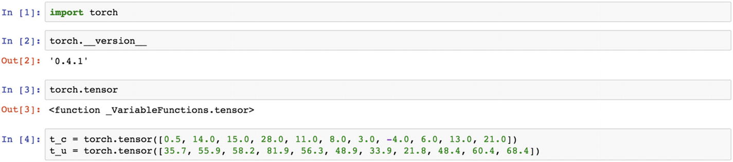
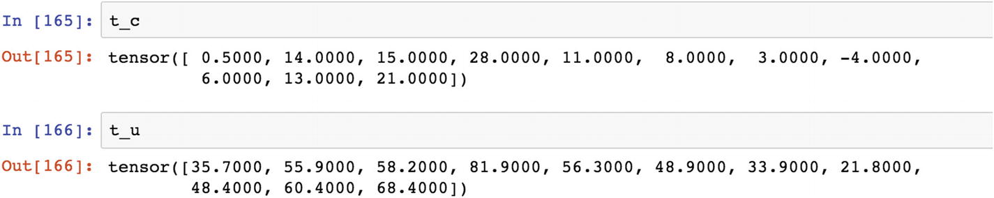
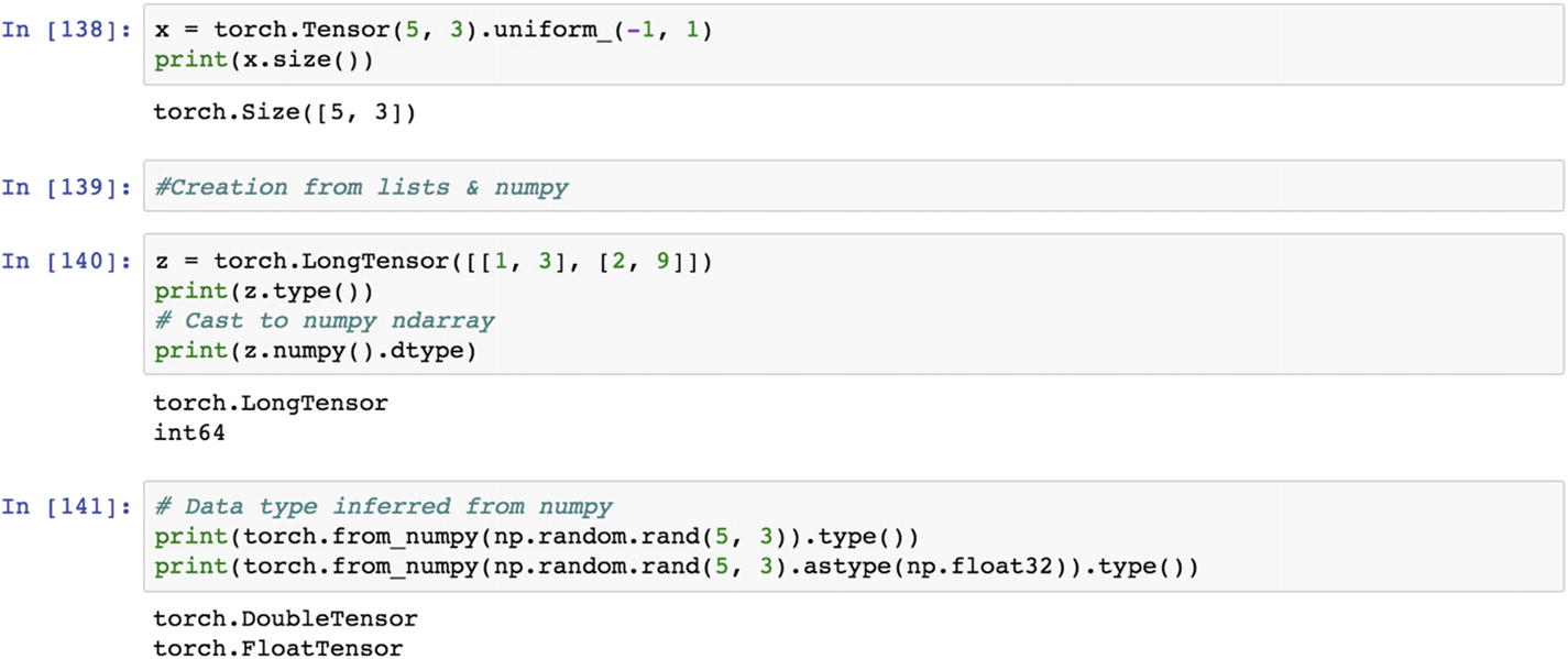
In the following example, t_c and t_u are two tensors. This can be constructed from any NumPy array.
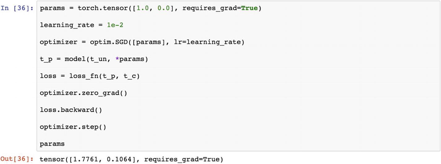
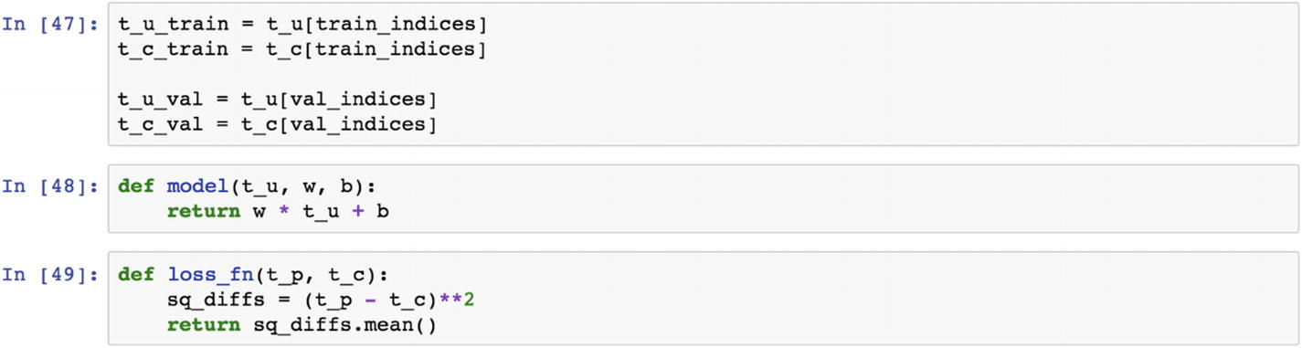
The sample model is just a linear equation to make the calculation happen and the loss function defined if the mean square error (MSE) shown next. Going forward in this chapter, we will increase the complexity of the model. For now, this is just a simple linear equation computation.
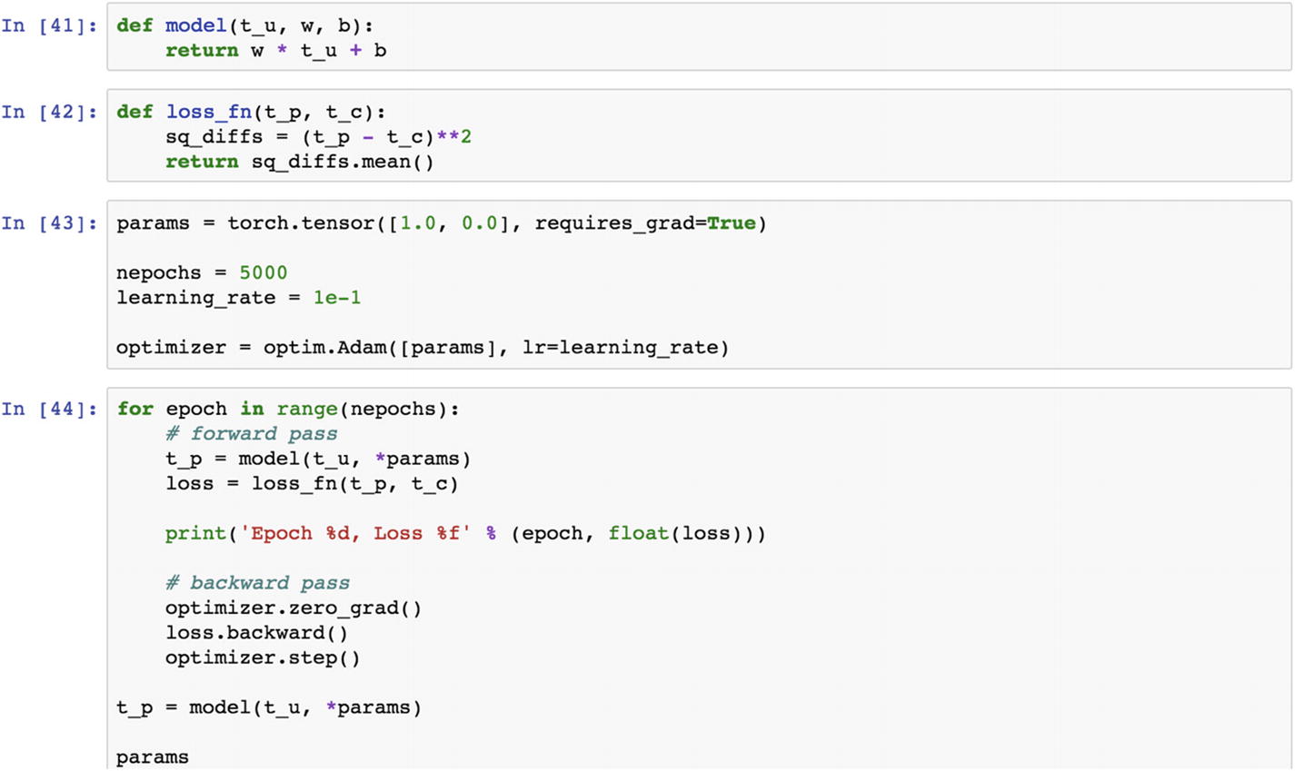
Let’s now define the model. The w parameter is the weight tensor, which is multiplied with the t_u tensor. The result is added with a constant tensor, b, and the loss function chosen is a custom-built one; it is also available in PyTorch. In the following example, t_u is the tensor used, t_p is the tensor predicted, and t_c is the precomputed tensor, with which the predicted tensor needs to be compared to calculate the loss function.
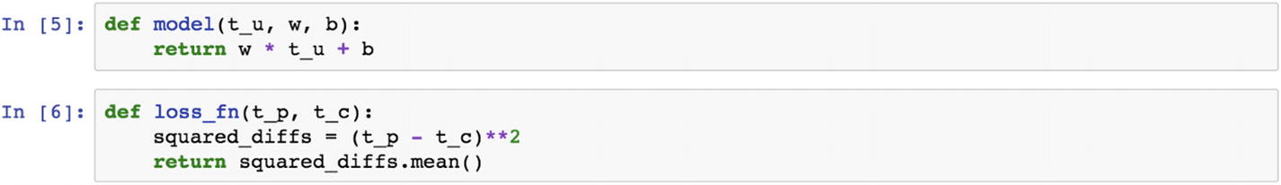
The formula w * t_u + b is the linear equation representation of a tensor-based computation.
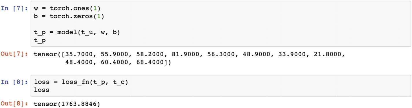
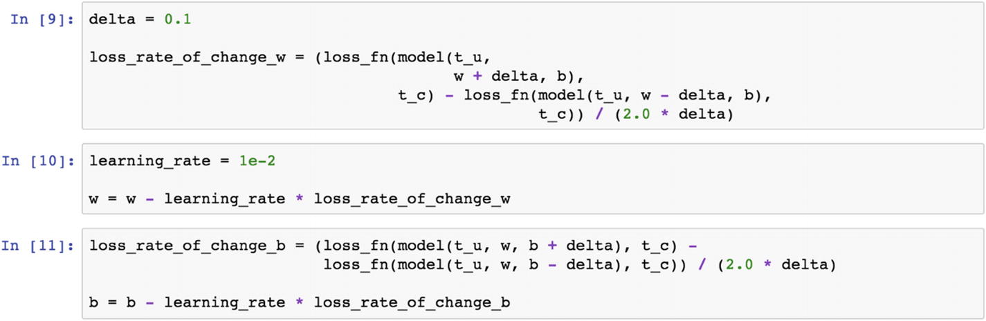
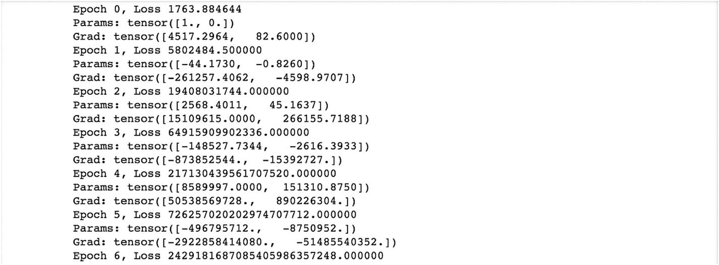
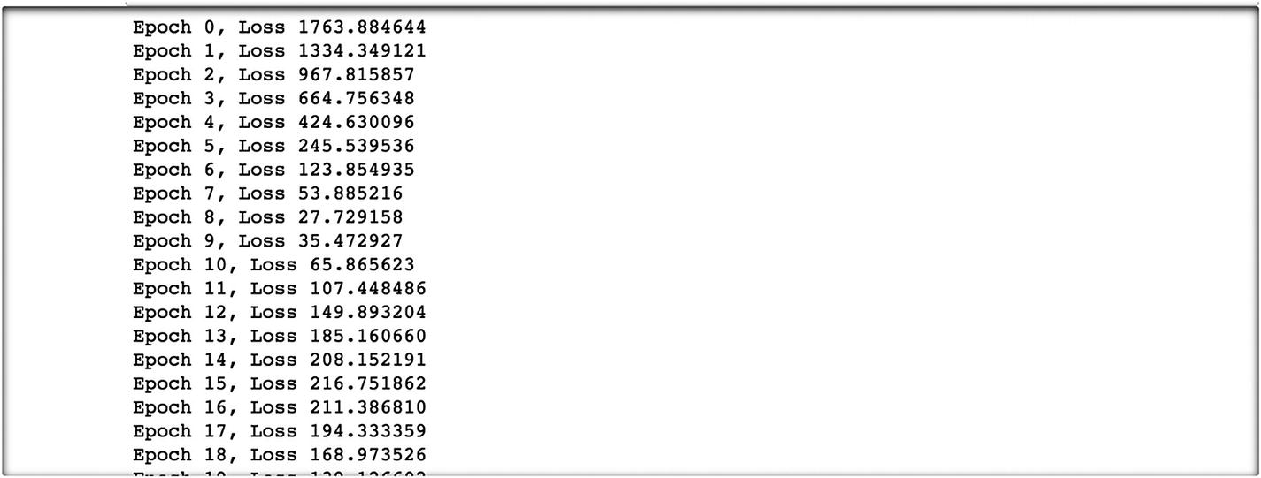
The initial loss value is 1763.88, which is too high because of the initial round of weights chosen. The error in the first round of iteration is backpropagated to reduce the errors in the second round, for which the initial set of weights needs to be updated. Therefore, the rate of change in the loss function is essential in updating the weights in the estimation process.
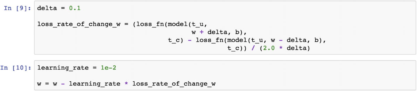
There are two parameters to update the rate of loss function: the learning rate at the current iteration and the learning rate at the previous iteration. If the delta between the two iterations exceeds a certain threshold, then the weight tensor needs to be updated, else model convergence could happen. The preceding script shows the delta and learning rate values. Currently, these are static values that the user has the option to change.

This is how a simple mean square loss function works in a two-dimensional tensor example, with a tensor size of 10,5.
Let’s look at the following example. The MSELoss function is within the neural network module of PyTorch.
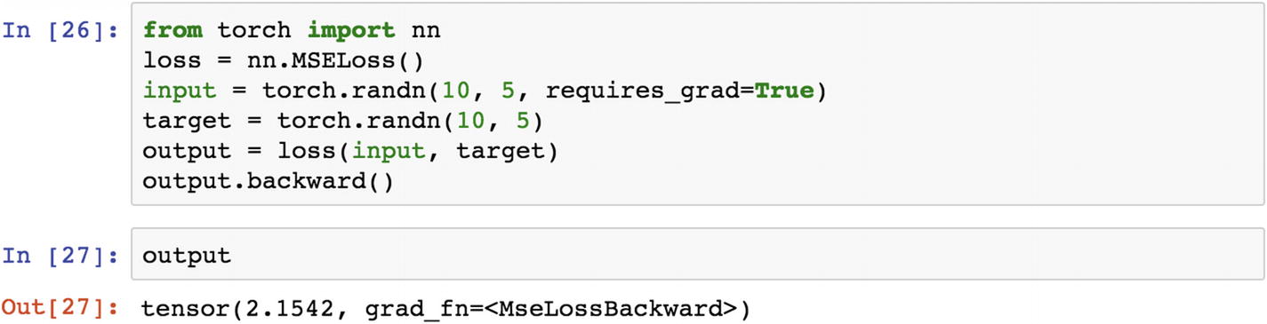
When we look at the gradient calculation that is used for backpropagation, it is shown as MSELoss.

Recipe 3-2. Estimating the Derivative of the Loss Function
Problem
How do we estimate the derivative of a loss function?
Solution
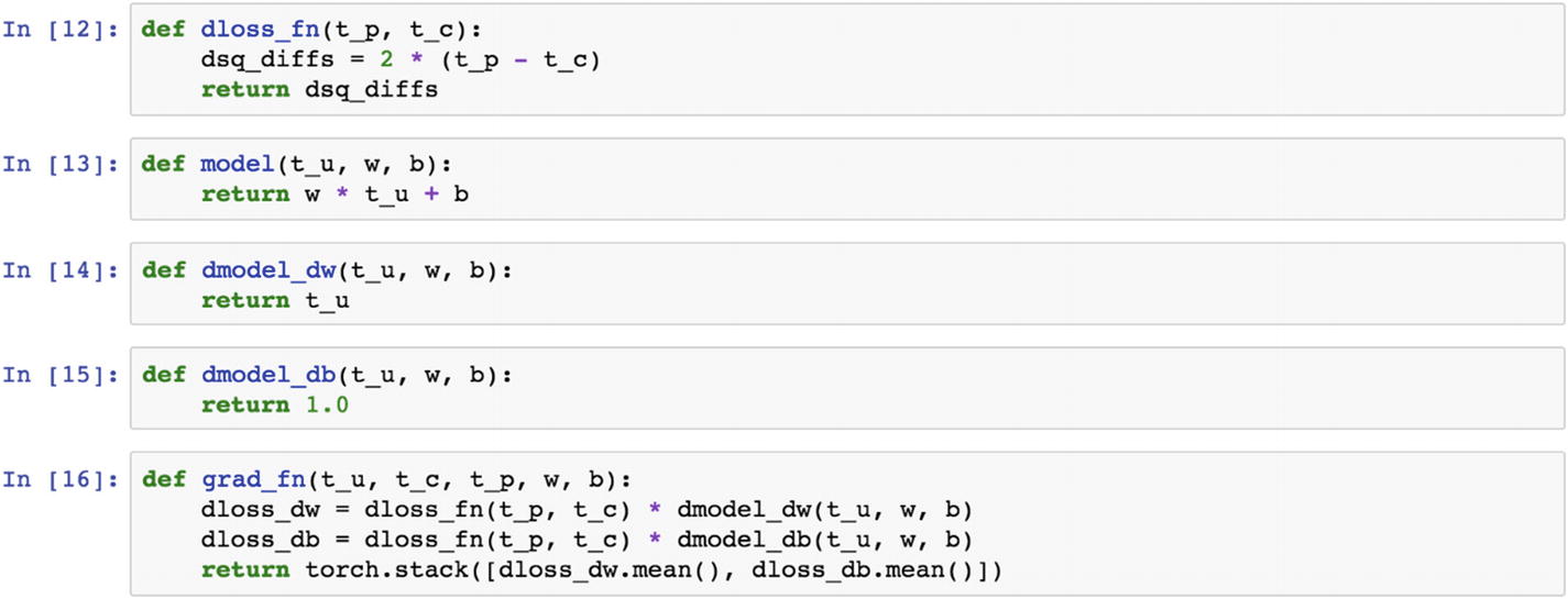
Using the following example, we change the loss function to two times the differences between the input and the output tensors, instead of MSELoss function. The following grad_fn, which is defined as a custom function, shows the user how the final output retrieves the derivative of the loss function.
How It Works
Let’s look at the following example. In the previous recipe, the last line of the script shows the grad_fn as an object embedded in the output object tensor. In this recipe, we explain how this is computed. grad_fn is a derivative of the loss function with respect to the parameters of the model. This is exactly what we do in the following grad_fn.
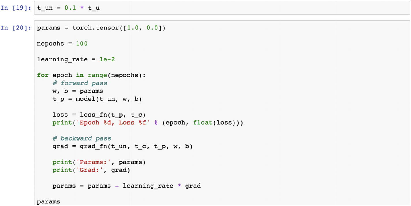
The parameters are the input, bias settings, and the learning rate, and the number of epochs for the model training. The estimation of these parameters provides values to the equation.
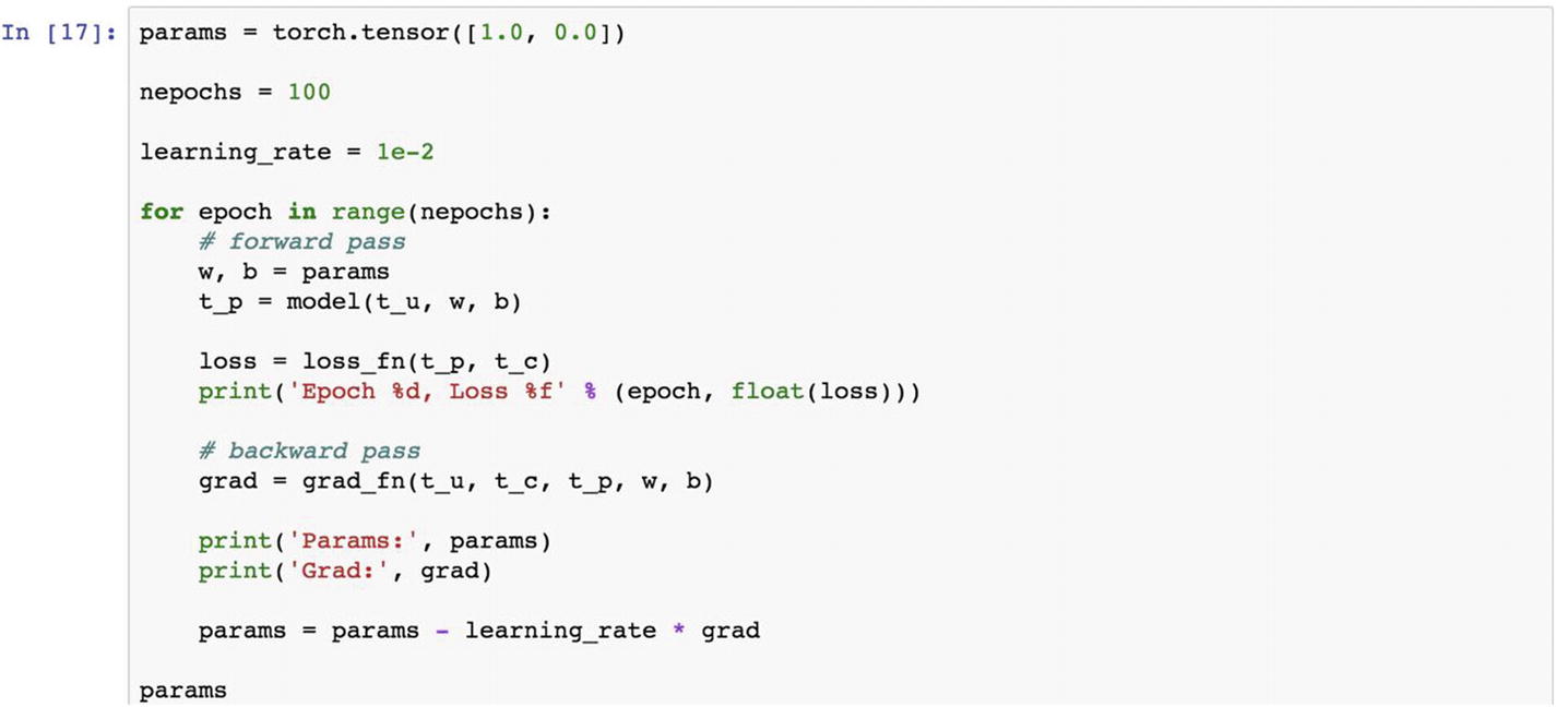
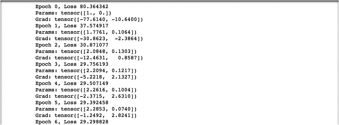
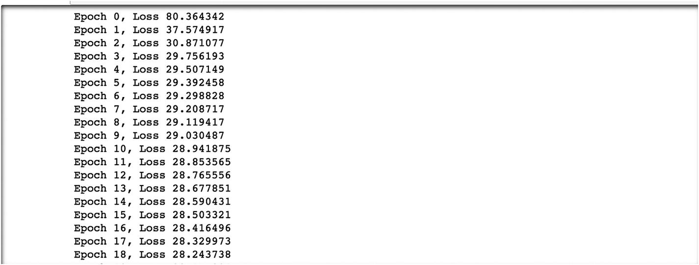
This is what the initial result looks like. Epoch is an iteration that produces a loss value from the loss function defined earlier. The params vector is about coefficients and constants that need to be changed to minimize the loss function. The grad function computes the feedback value to the next epoch. This is just an example. The number of epochs chosen is an iterative task depending on the input data, output data, and choice of loss and optimization functions.
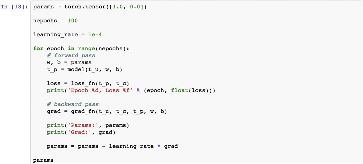
If we reduce the learning rate, we are able to pass relevant values to the gradient, the parameter updates in a better way, and model convergence becomes quicker.
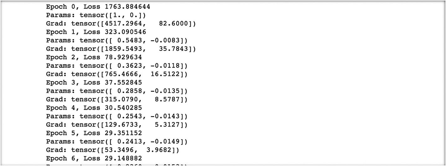
The initial results look like as the following. The results are at epoch 5 and the loss value is 29.35, which is much lower than 1763.88 at epoch 0, and corresponding to the epoch, the estimated parameters are 0.24 and –.01, at epoch 100. These parameter values are optimal.
If we reduce the learning rate a bit, then the process of weight updating will be a little slower, which means that the epoch number needs to be increased in order to find a stable state for the model.
The following are the results that we observe.
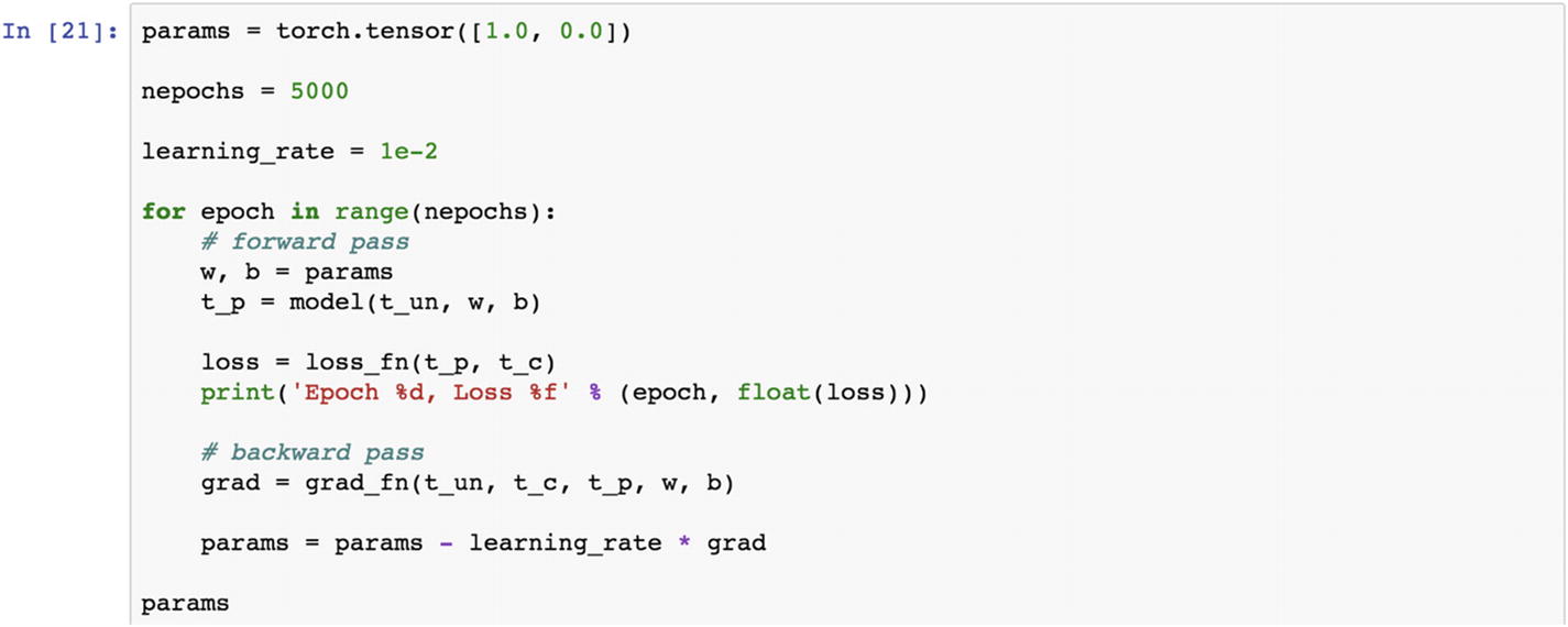
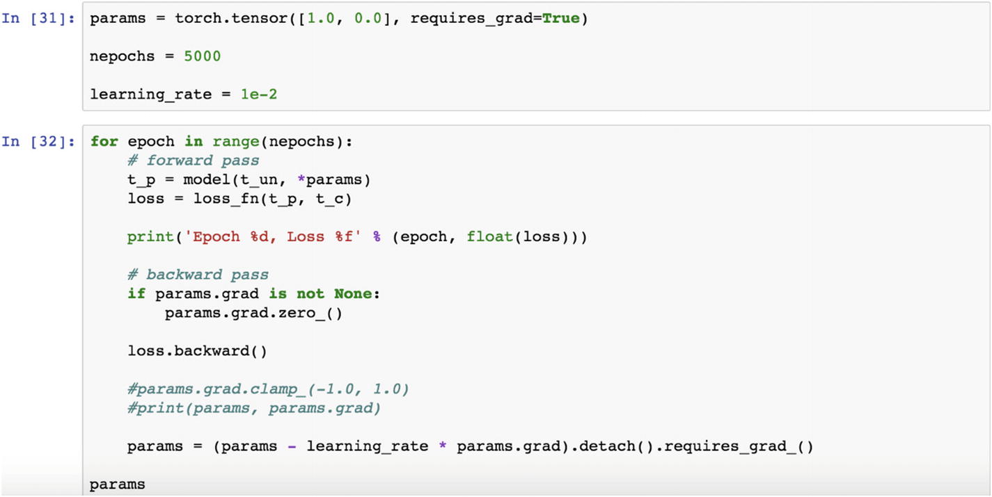
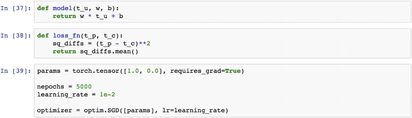
If we increase the number of epochs, then what happens to the loss function and parameter tensor can be viewed in the following script, in which we print the loss value to find the minimum loss corresponding to the epoch. Then we can extract the best parameters from the model.
The following are the results.
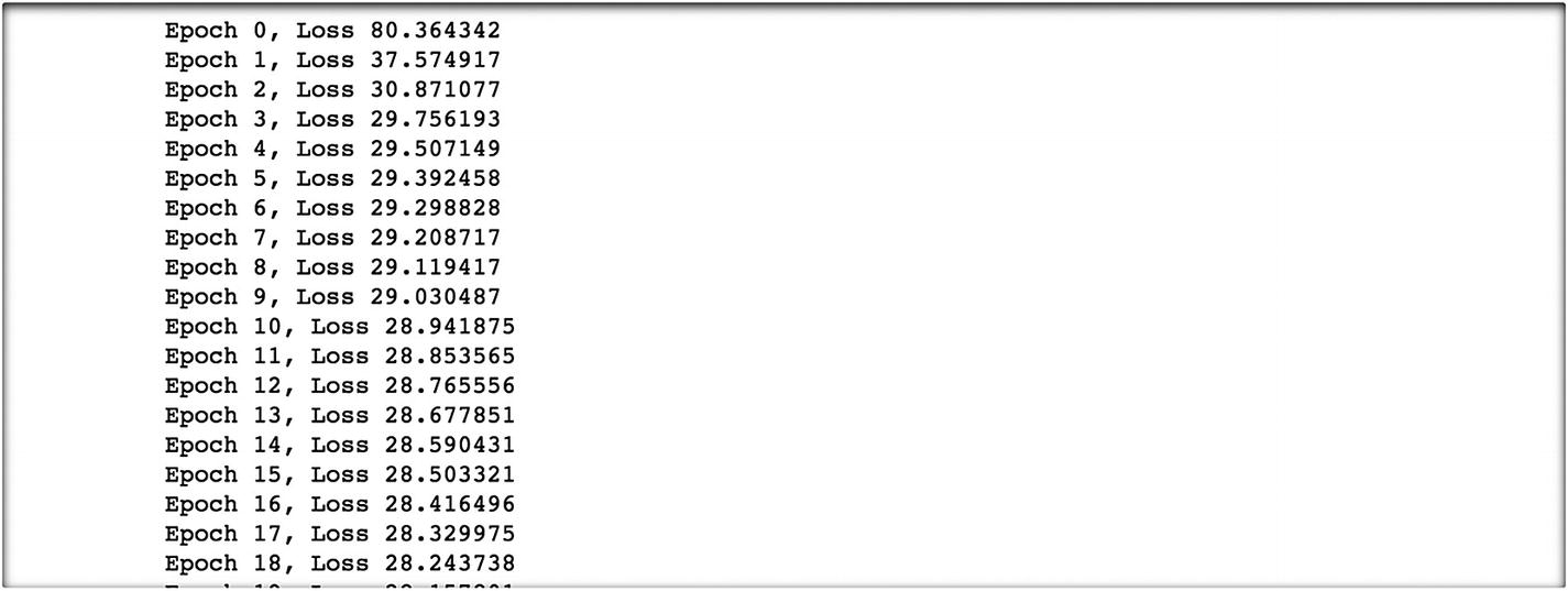
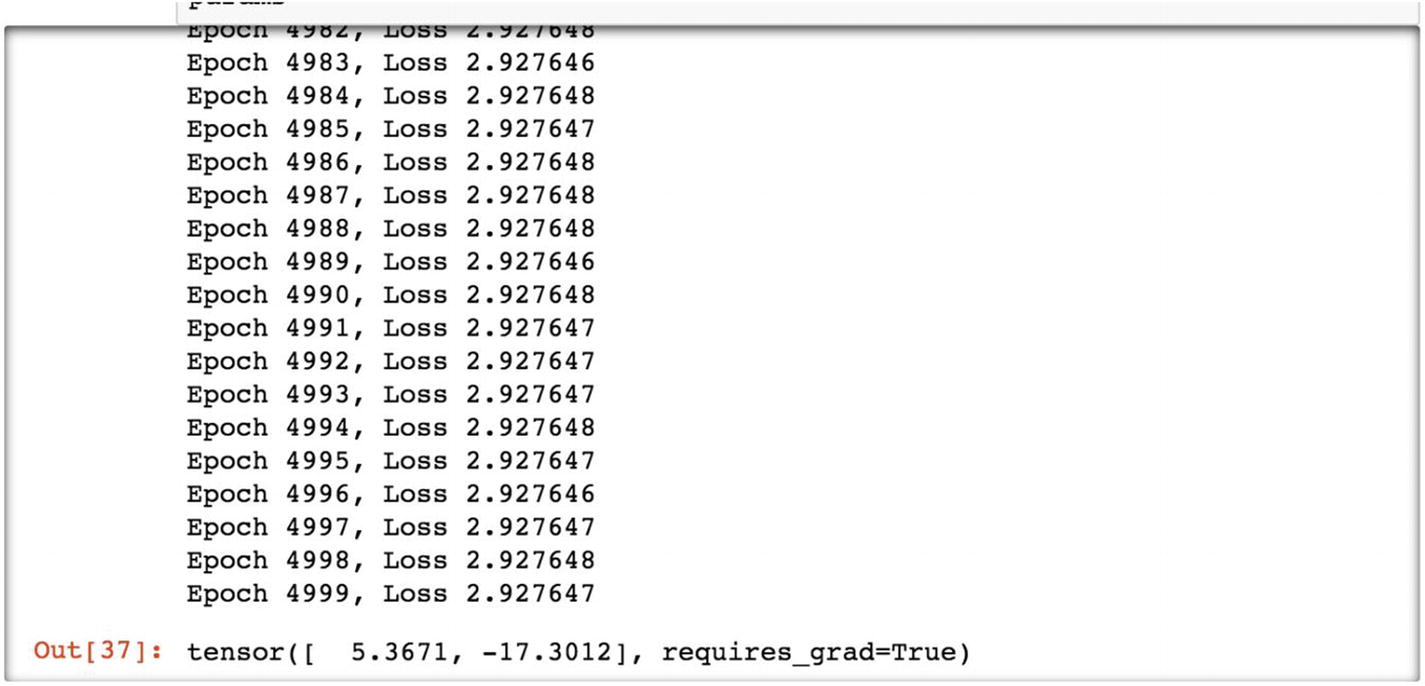
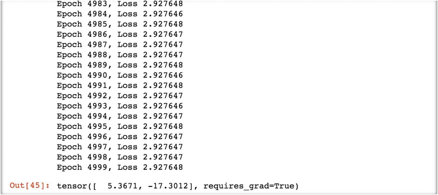
The following is the final loss value at the final epoch level.
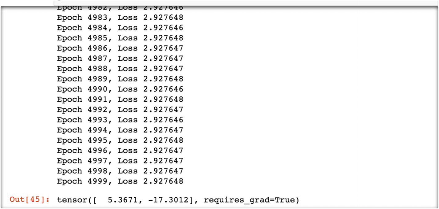
At epoch 5000, the loss value is 2.92, which is not going down further; hence, at this iteration level, the tensor output displays 5.36 as the final weight and –17.30 as the final bias. These are the final parameters from the model.
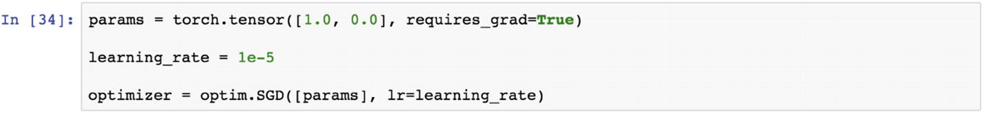
To fine-tune this model in estimating parameters, we can redefine the model and the loss function and apply it to the same example.


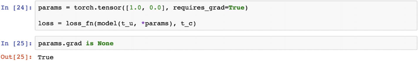
Set up the parameters. After completing the training process, we should reset the grad function to None.
Recipe 3-3. Fine-Tuning a Model
Problem
How do we find the gradients of the loss function by applying an optimization function to optimize the loss function?
Solution
We’ll use the backward() function.
How It Works
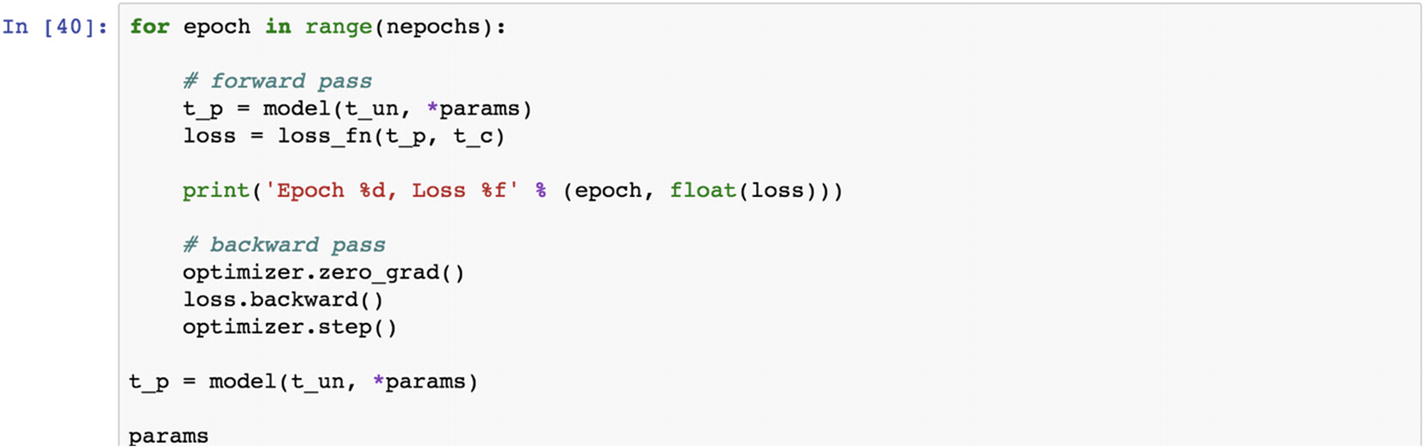
Let’s look at the following example. The backward() function calculates the gradients of a function with respect to its parameters. In this section, we retrain the model with new set of hyperparameters.
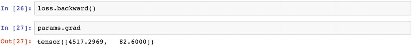
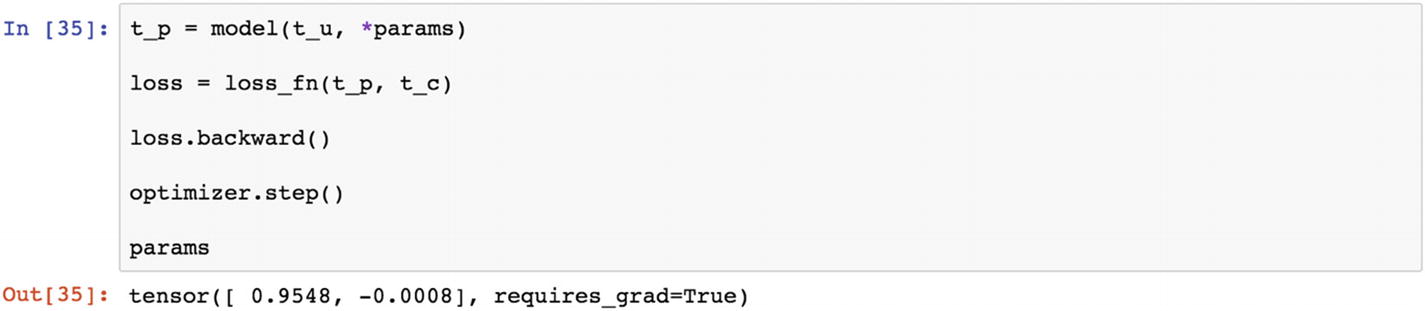
Reset the parameter grid. If we do not o reset the parameters in an existing session, the error values accumulated from any other session become mixed, so it is important to reset the parameter grid.
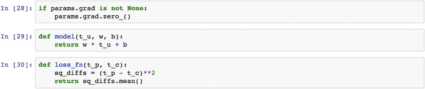
After redefining the model and the loss function, let’s retrain the model.
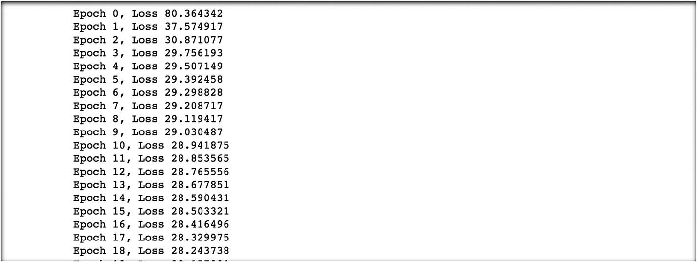
We have taken 5000 epochs. We train the parameters in a backward propagation method and get the following results. At epoch 0, the loss value is 80.36. We try to minimize the loss value as we proceed with the next iteration by adjusting the learning rate. At the final epoch, we observe that the loss value is 2.92, which is same result as before but with a different loss function and using backpropagation.
The final model parameters are 5.3671 with a bias of –17.3012.
Recipe 3-4. Selecting an Optimization Function
Problem
How do we optimize the gradients with the function in Recipe 3-3?
Solution
There are certain functions that are embedded in PyTorch, and there are certain optimization functions that the user has to create.
How It Works
Let’s look at the following example.
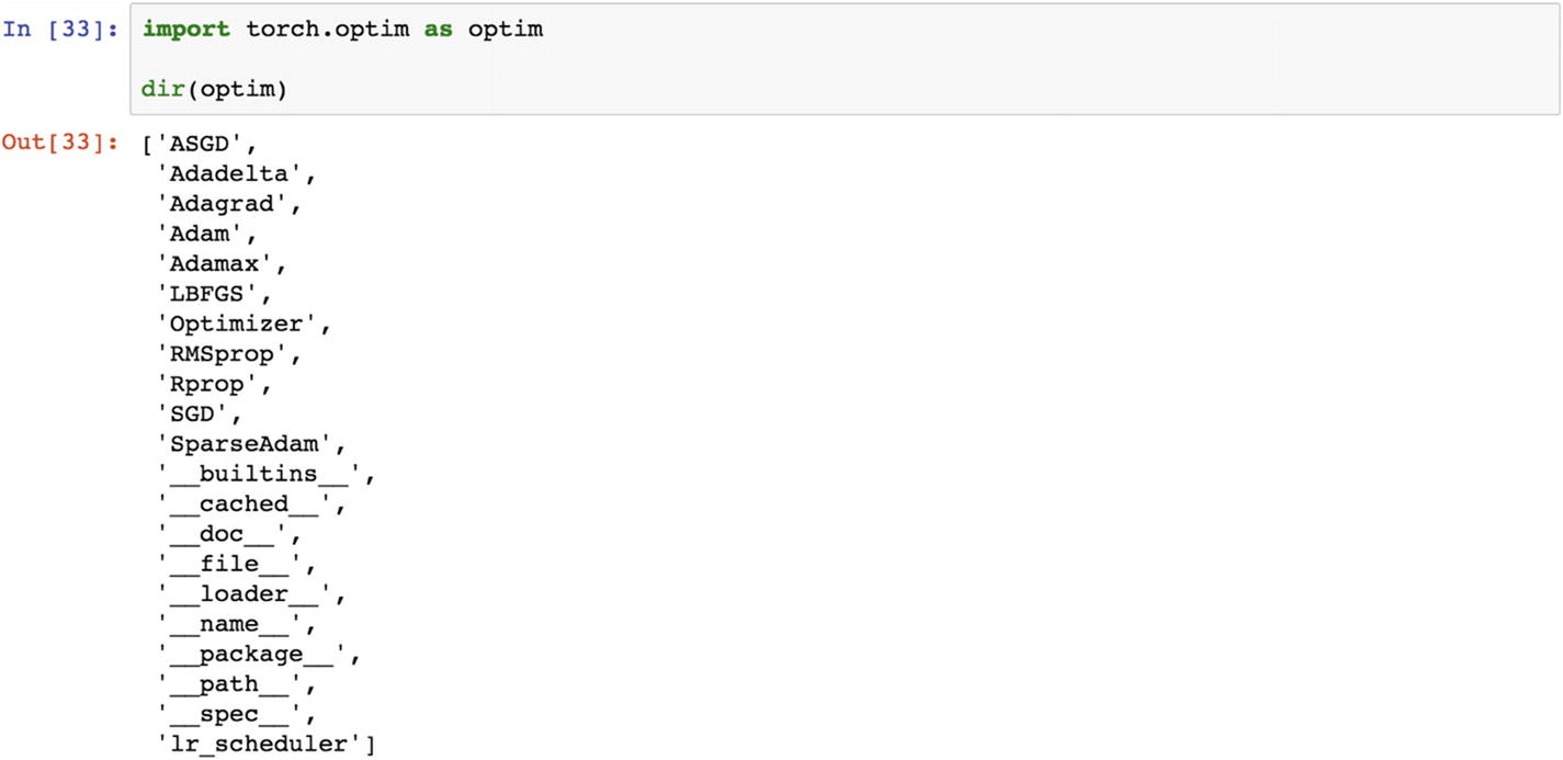
Each optimization method is unique in solving a problem. We will describe it later.
The Adam optimizer is a first-order, gradient-based optimization of stochastic objective functions. It is based on adaptive estimation of lower-order moments. This is computationally efficient enough for deployment on large datasets. To use torch.optim, we have to construct an optimizer object in our code that will hold the current state of the parameters and will update the parameters based on the computed gradients, moments, and learning rate. To construct an optimizer, we have to give it an iterable containing the parameters and ensure that all the parameters are variables to optimize. Then, we can specify optimizer-specific options, such as the learning rate, weight decay, moments, and so forth.
Adadelta is another optimizer that is fast enough to work on large datasets. This method does not require manual fine-tuning of the learning rate; the algorithm takes care of it internally.
Now let’s call the model and loss function out once again and apply them along with the optimization function.
Let’s look at the gradient in a loss function. Using the optimization library, we can try to find the best value of the loss function.
The example has two custom functions and a loss function. We have taken two small tensor values. The new thing is that we have taken the optimizer to find the minimum value.
In the following example, we have chosen Adam as the optimizer.
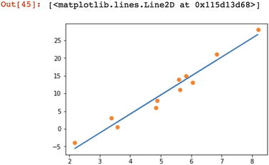
In the preceding code, we computed the optimized parameters and computed the predicted tensors using the actual and predicted tensors. We can display a graph that has a line shown as a regression line.
Let’s visualize the sample data in graphical form using the actual and predicted tensors.

Recipe 3-5. Further Optimizing the Function
Problem
How do we optimize the training set and test it with a validation set using random samples?
Solution
We’ll go through the process of further optimization.
How It Works
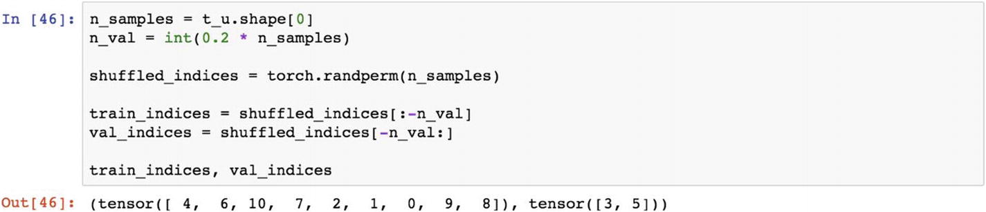
Let’s look at the following example. Here we set the number of samples, then we take 20% of the data as validation samples using shuffled_indices. We took random samples of all the records. The objective of the train and validation set is to build a model in a training set, make the prediction on the validation set, and check the accuracy of the model.
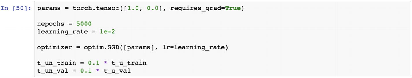
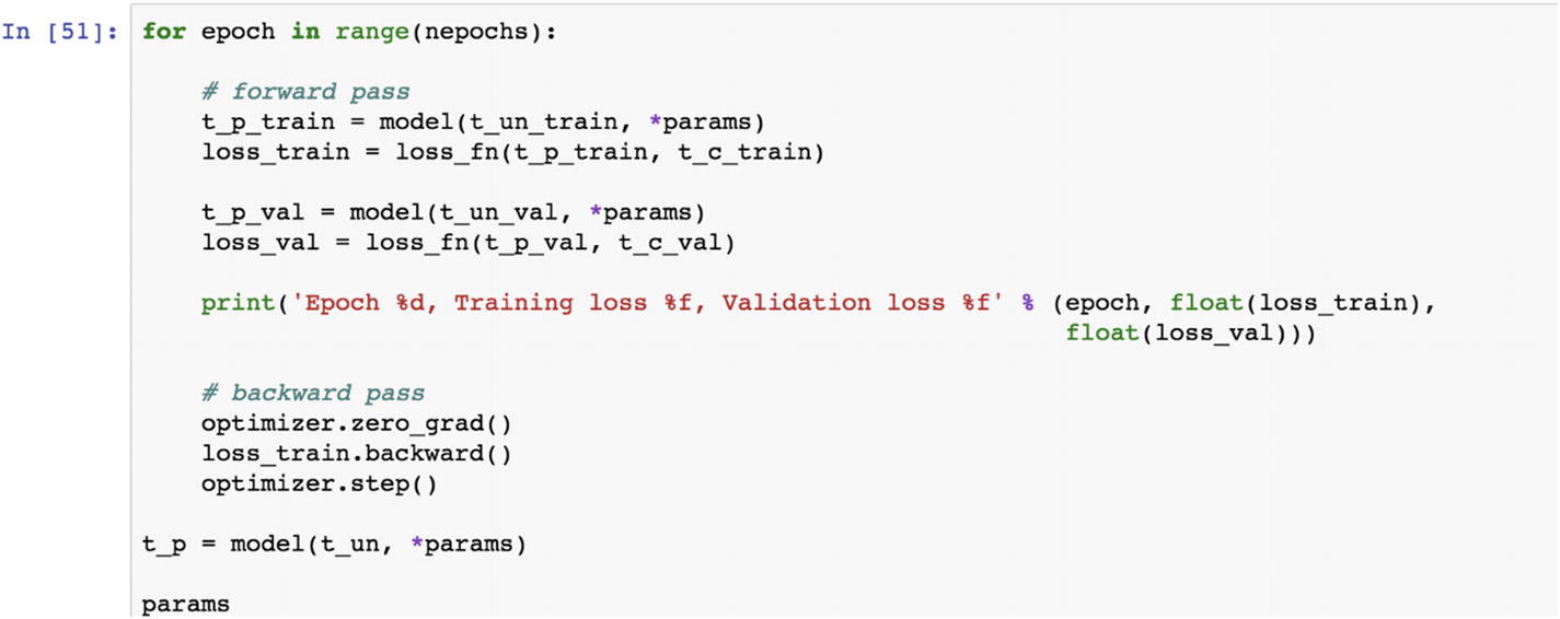
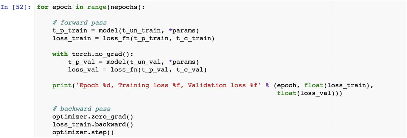
Now let’s run the train and validation process. We first take the training input data and multiply it by the parameter’s next line. We make a prediction and compute the loss function. Using the same model in third line, we make predictions and then we evaluate the loss function for the validation dataset. In the backpropagation process, we calculate the gradient of the loss function for the training set, and using the optimizer, we update the parameters.
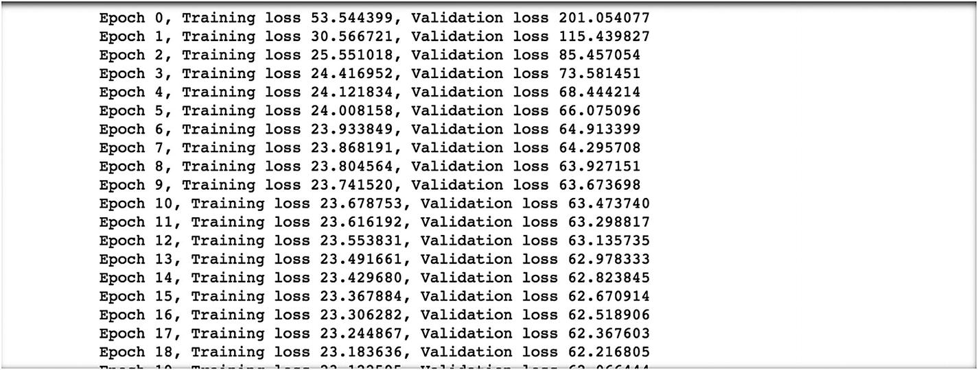
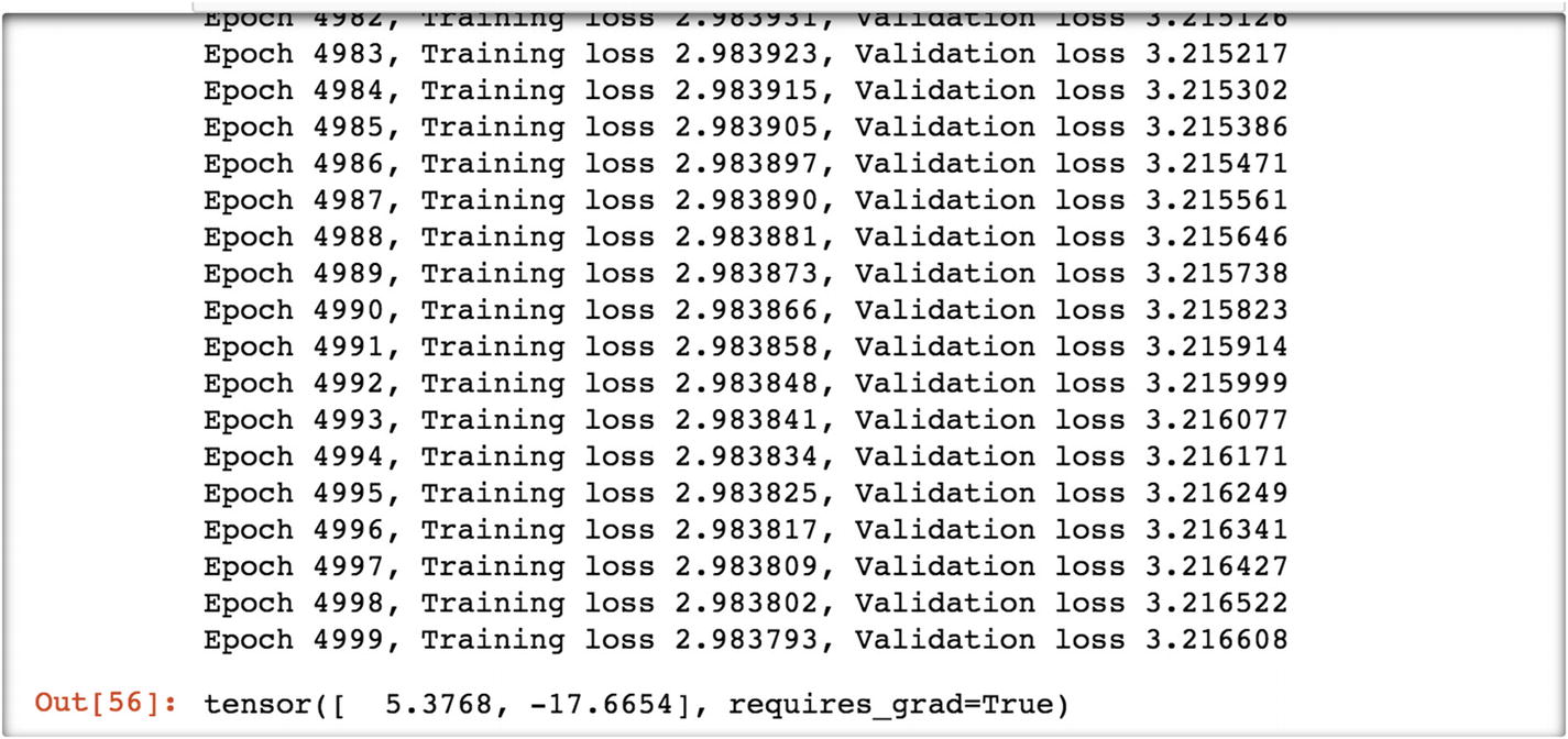
The following are the last 10 epochs and their results.
In the previous step, the gradient was set to true. In the following set, we disable gradient calculation by using the torch.no_grad() function . The rest of the syntax remains same. Disabling gradient calculation is useful for drawing inferences, when we are sure that we will not call Tensor.backward() . This reduces memory consumption for computations that would otherwise be requires_grad=True.
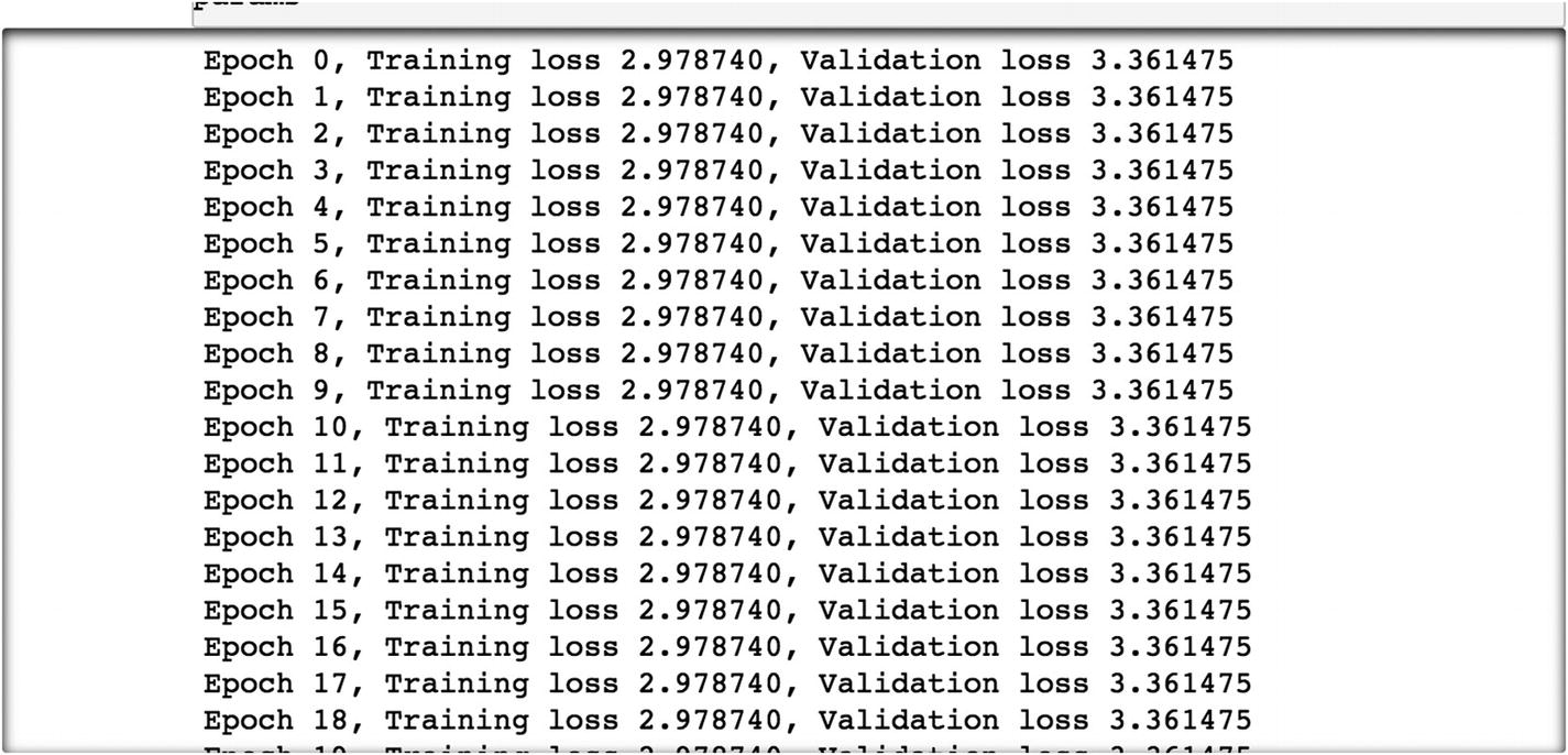
The last rounds of epochs are displayed in other lines of code, as follows.
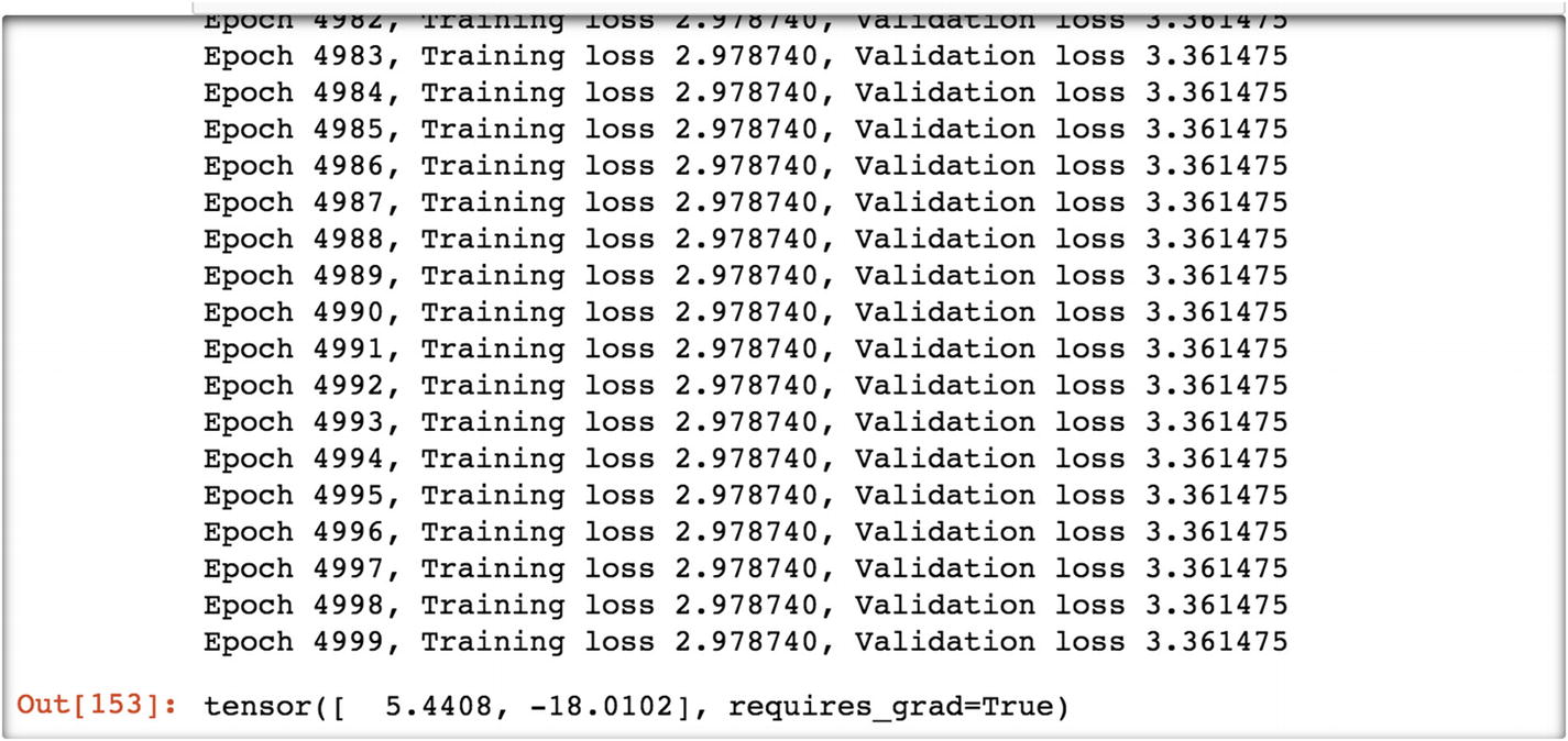
The final parameters are 5.44 and –18.012.
Recipe 3-6. Implementing a Convolutional Neural Network (CNN)
Problem
How do we implement a convolutional neural network using PyTorch?
Solution
There are various built-in datasets available on torchvision. We are considering the MNIST dataset and trying to build a CNN model.
How It Works
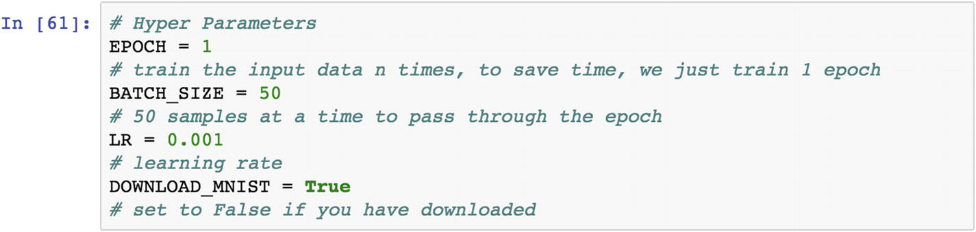
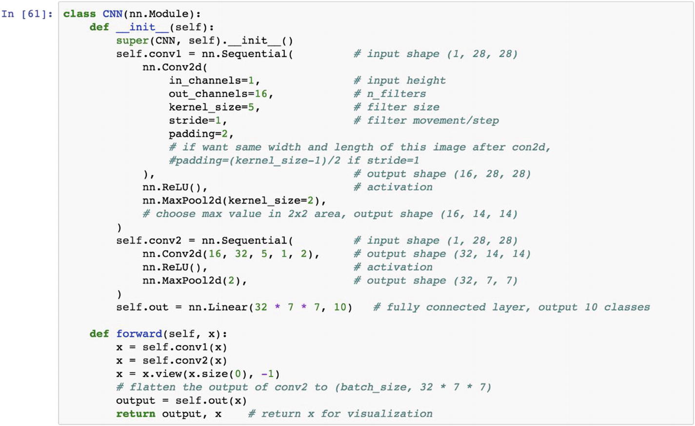
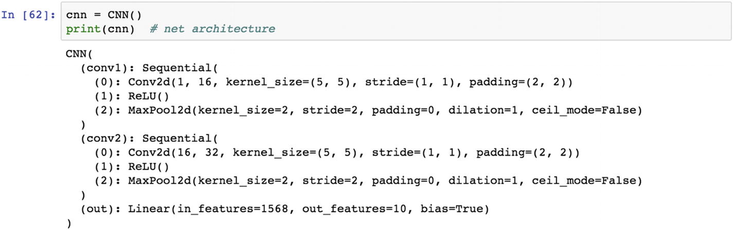
Let’s look at the following example. As a first step, we set up the hyperparameters . The second step is to set up the architecture. The last step is to train the model and make predictions.
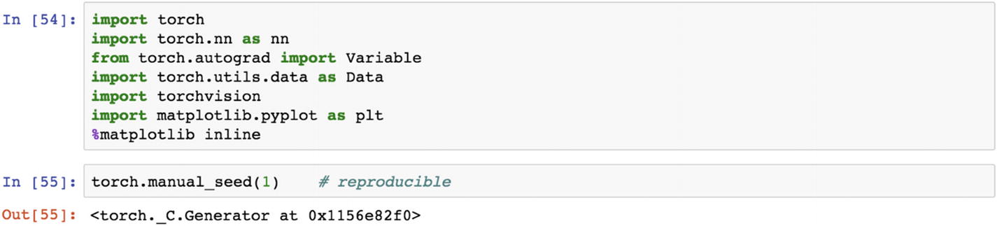
In the preceding code, we are importing the necessary libraries for deploying the convolutional neural network model using the digits dataset. The MNIST digits dataset is the most popular dataset in deep learning for computer vision and image processing.
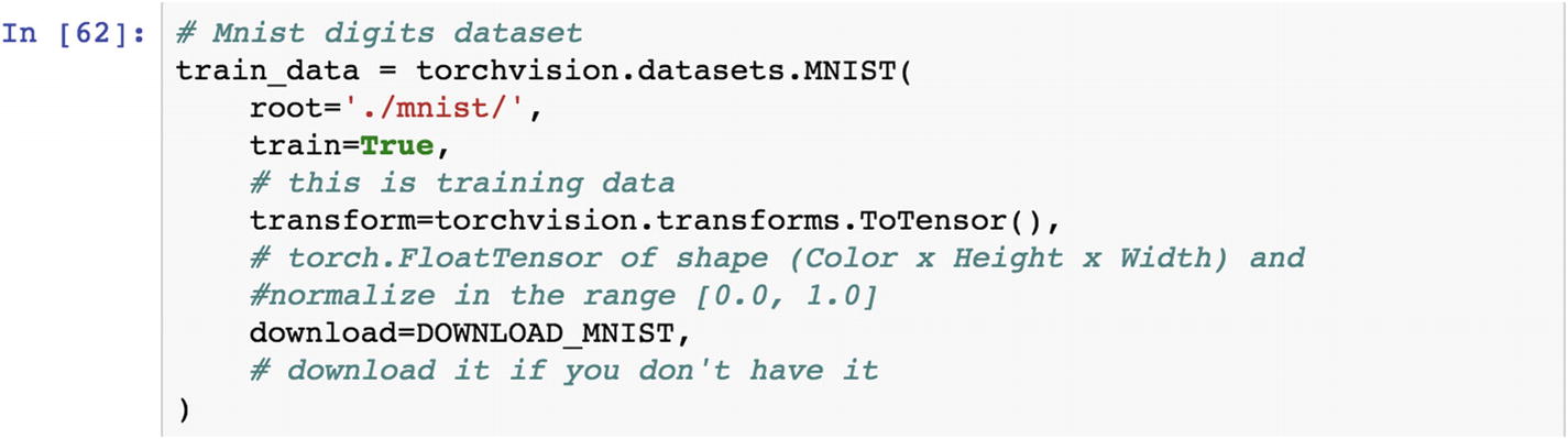
Let’s load the dataset using the loader functionality .
In convolutional neural network architecture, the input image is converted to a feature set as set by color times height and width of the image. Because of the dimensionality of the dataset, we cannot model it to predict the output. The output layer in the preceding graph has classes such as car, truck, van, and bicycle. The input bicycle image has features that the CNN model should make use of and predict it correctly. The convolution layer is always accompanied by the pooling layer, which can be max pooling and average pooling. The different layers of pooling and convolution continue until the dimensionality is reduced to a level where we can use fully connected simple neural networks to predict the correct classes.

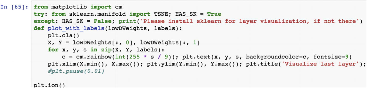
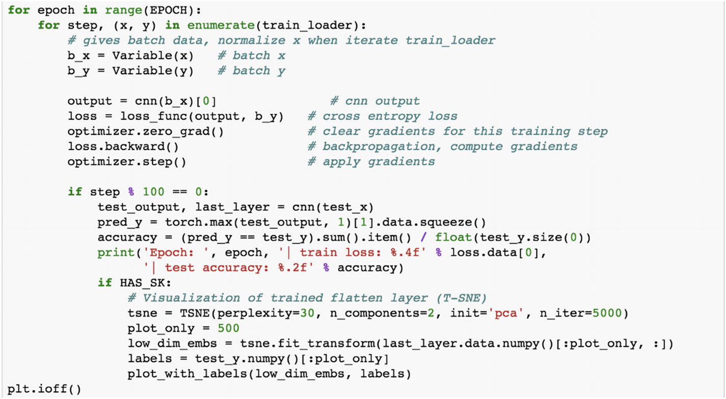
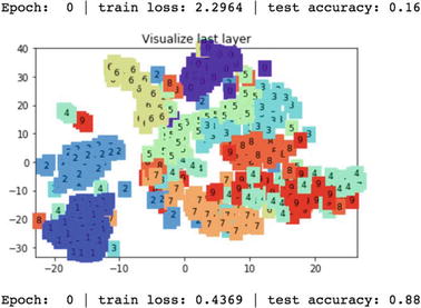
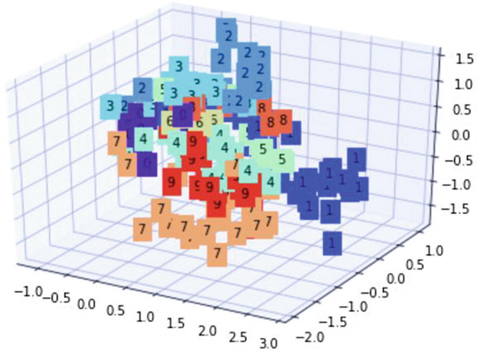
In the preceding graph, if we look at the number 4, it is scattered throughout the graph. Ideally, all of the 4s are closer to each other. This is because the test accuracy was very low.
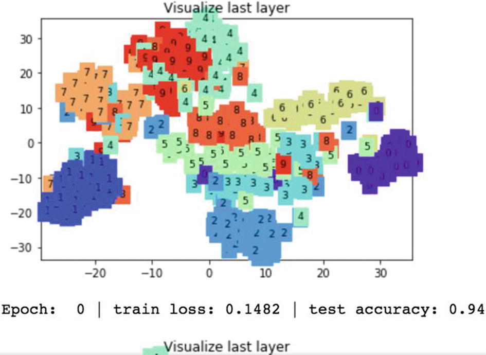
In this iteration, the training loss is reduced from 0.4369 to 0.1482 and the test accuracy improves from 16% to 94%. The digits with the same color are placed closely on the graph.
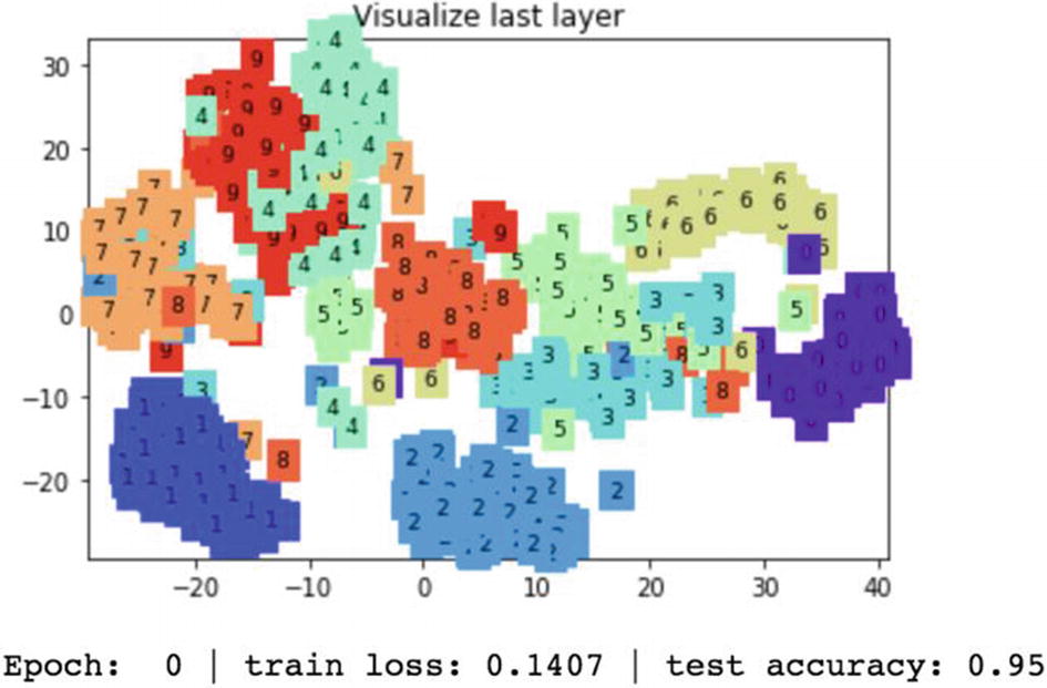
In the next epoch, the test accuracy on the MNIST digits dataset the accuracy increases to 95%.
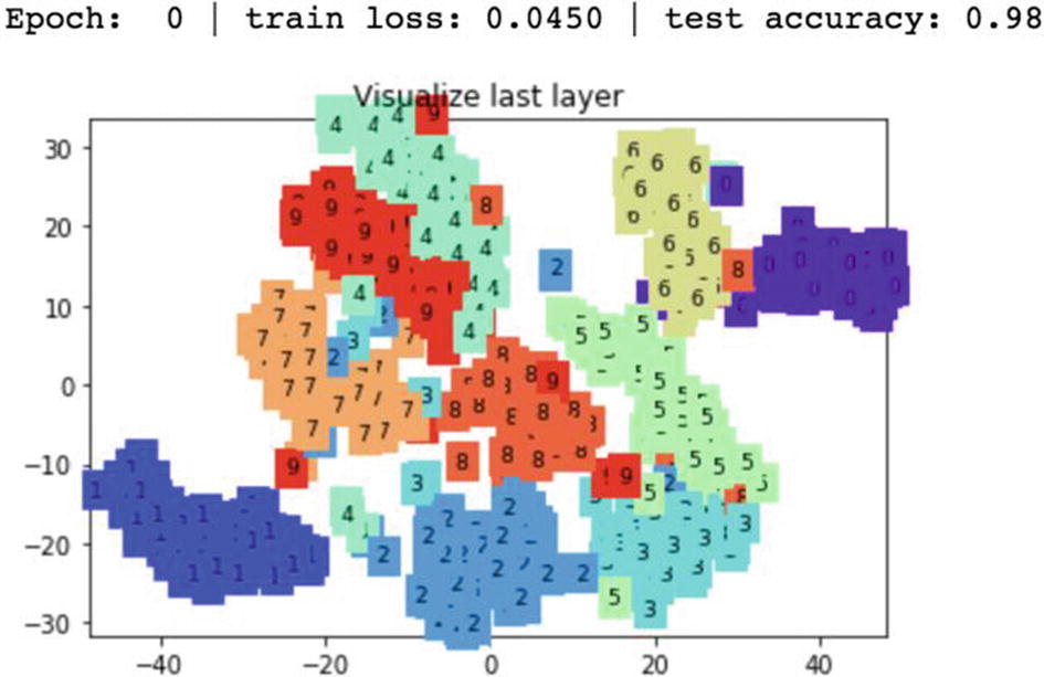
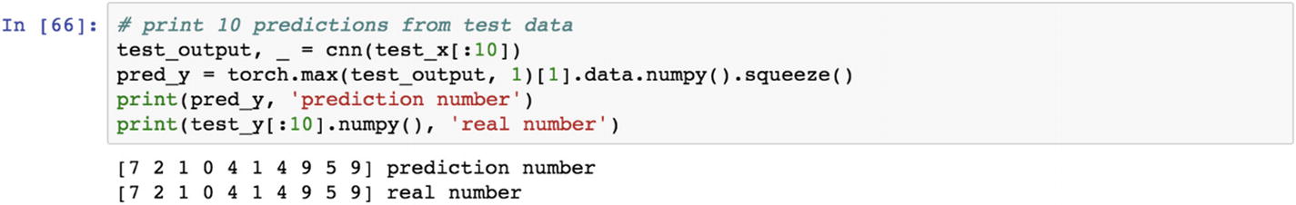
In the final step/epoch, the digits with similar numbers are placed together. After training a model successfully, the next step is to make use of the model to predict. The following code explains the predictions process. The output object is numbered as 0, 1, 2, and so forth. The following shows the real and predicted numbers.
Recipe 3-7. Reloading a Model
Problem
How do we store and re-upload a model that has already been trained? Given the nature of deep learning models, which typically require a larger training time, the computational process creates a huge cost to the company. Can we retrain the model with new inputs and store the model?
Solution
In the production environment, we typically cannot train and predict at the same time because the training process takes a very long time. The prediction services cannot be applied until the training process using epoch is completed, the prediction services cannot be applied. Disassociating the training process from the prediction process is required; therefore, we need to store the application’s trained model and continue until the next phase of training is done.
How It Works
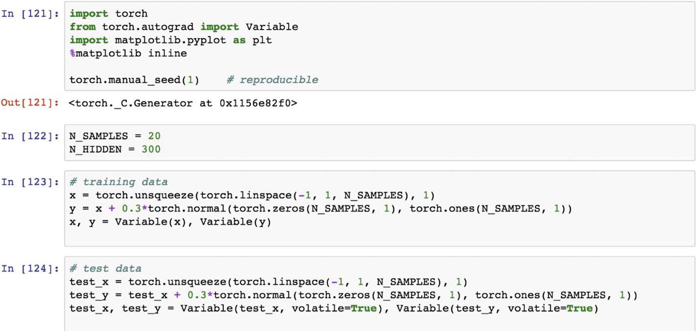
Let’s look at the following example, where we are creating the save function, which uses the Torch neural network module to create the model and the restore_net() function to get back the neural network model that was trained earlier.
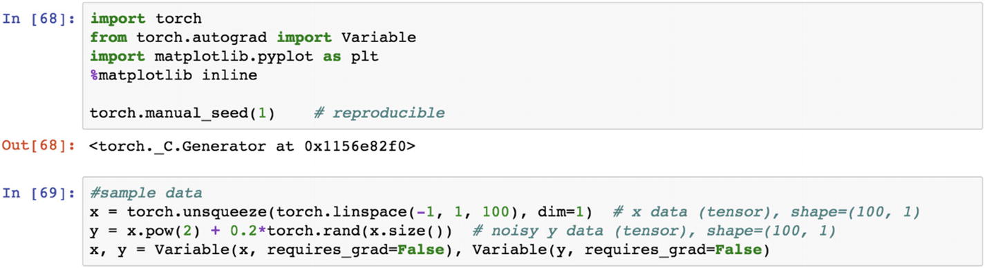
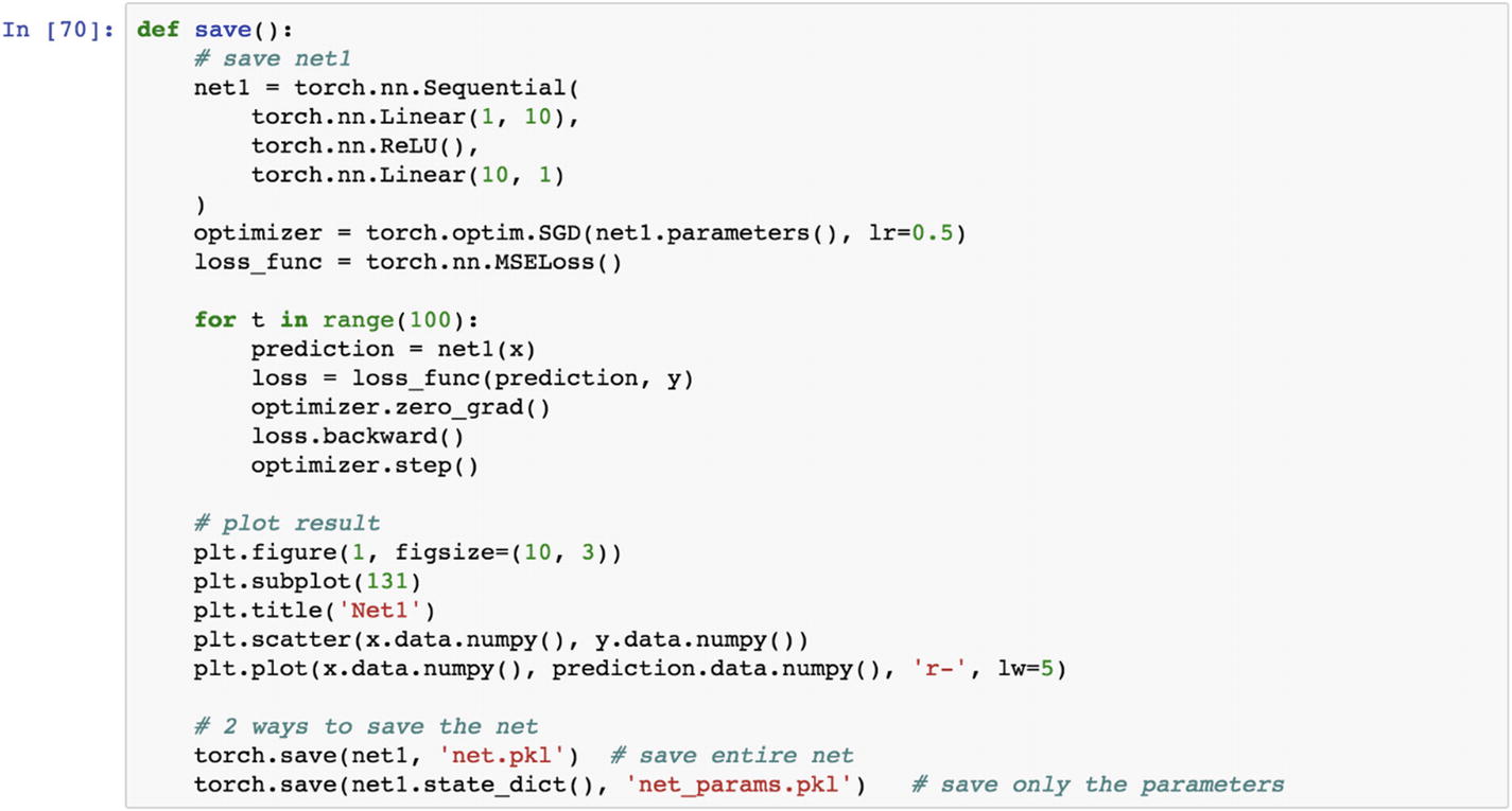
The preceding script contains a dependent Y variable and an independent X variable as sample data points to create a neural network model. The following save function stores the model. The net1 object is the trained neural network model, which can be stored using two different protocols: (1) save the entire neural network model with all the weights and biases, and (2) save the model using only the weights. If the trained model object is very heavy in terms of size, we should save only the parameters that are weights; if the trained object size is low, then the entire model can be stored.
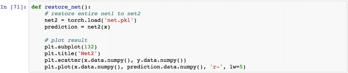
The prebuilt neural network model can be reloaded to the existing PyTorch session by using the load function. To test the net1 object and make predictions, we load the net1 object and store the model as net2. By using the net2 object, we can predict the outcome variable. The following script generates the graph as a dependent and an independent variable. prediction.data.numpy() in the last line of the code shows the predicted result.
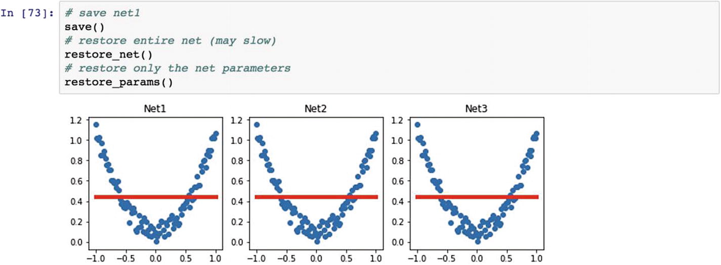
Loading the pickle file format of the entire neural network is relatively slow; however, if we are only making predictions for a new dataset, we can only load the parameters of the model in a pickle format rather than the whole network.
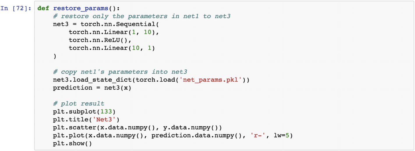
Reuse the model. The restore function makes sure that the trained parameters can be reused by the model. To restore the model, we can use the load_state_dict() function to load the parameters of the model. If we see the following three models in the graph, they are identical, because net2 and net3 are copies of net1.
Recipe 3-8. Implementing a Recurrent Neural Network (RNN)
Problem
How do we set up a recurrent neural network using the MNIST dataset?
Solution
The recurrent neural network is considered as a memory network. We will use the epoch as 1 and a batch size of 64 samples at a time to establish the connection between the input and the output. Using the RNN model, we can predict the digits present in the images.
How It Works
Let’s look at the following example. The recurrent neural network takes a sequence of vectors in the input layer and produces a sequence of vectors in the output layer. The information sequence is processed through the internal state transfer in the recurrent layer. Sometimes the output values have a long dependency in past historical values. This is another variant of the RNN model: the long short-term memory (LSTM) model . This is applicable for any sort of domain where the information is consumed in a sequential manner; for example, in a time series where the current stock price is decided by the historical stock price, where the dependency can be short or long. Similarly, the context prediction using the long and short range of textual input vectors. There are other industry use cases, such as noise classification, where noise is also a sequence of information.
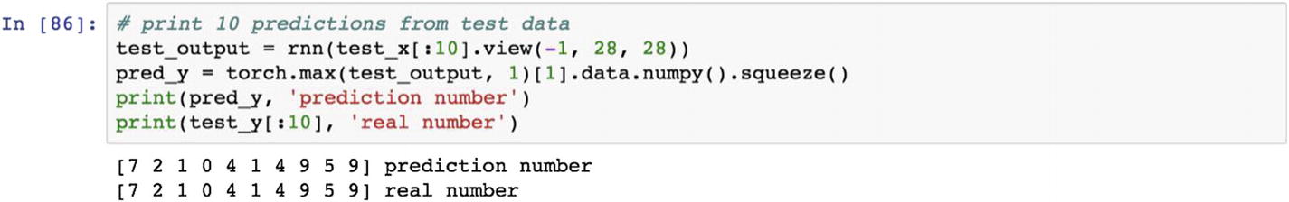
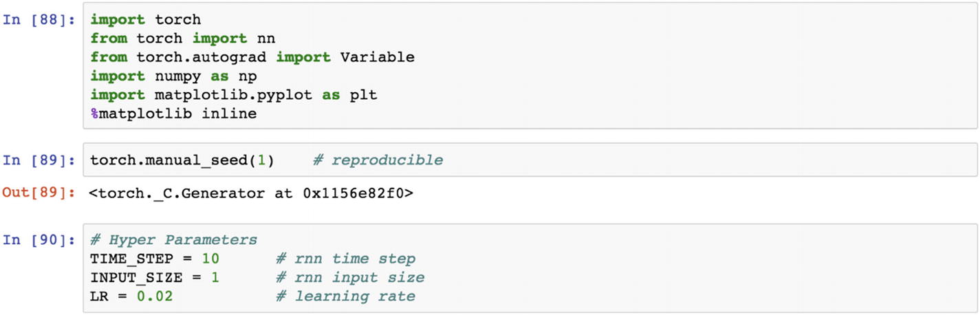
The following piece of code explains the execution of RNN model using PyTorch module.
There are three sets of weights: U, V and W. The set of weights vector, represented by W, is for passing information among the memory cells in the network that display communication among the hidden state. RNN uses an embedding layer using the Word2vec representation. The embedding matrix is the size of the number of words by the number of neurons in the hidden layer. If you have 20,000 words and 1000 hidden units, for example, the matrix has a 20,000×1000 size of the embedding layer. The new representations are passed to LSTM cells, which go to a sigmoid output layer.
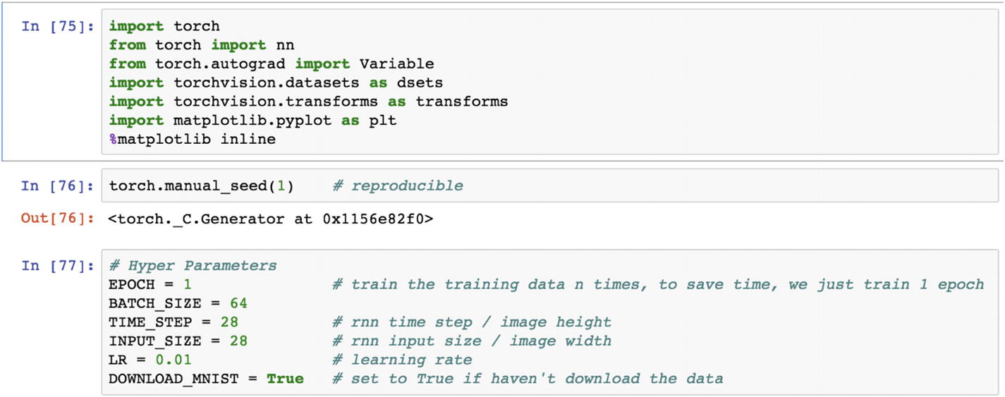
The RNN models have hyperparameters, such as the number of iterations (EPOCH); batch size dependent on the memory available in a single machine; a time step to remember the sequence of information; input size, which shows the vector size; and learning rate. The selection of these values is indicative; we cannot depend on them for other use cases. The value selection for hyperparameter tuning is an iterative process; either you can choose multiple parameters and decide which one is working, or do parallel training of the model and decide which one is working fine.
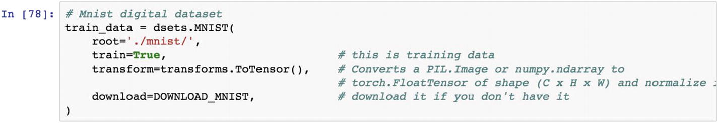
Using the dsets.MINIST() function, we can load the dataset to the current session. If you need to store the dataset, then download it locally.
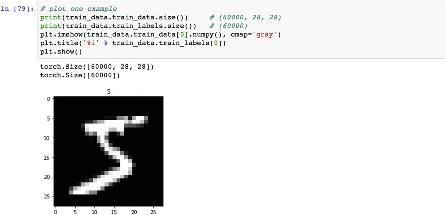
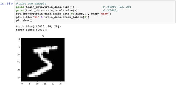
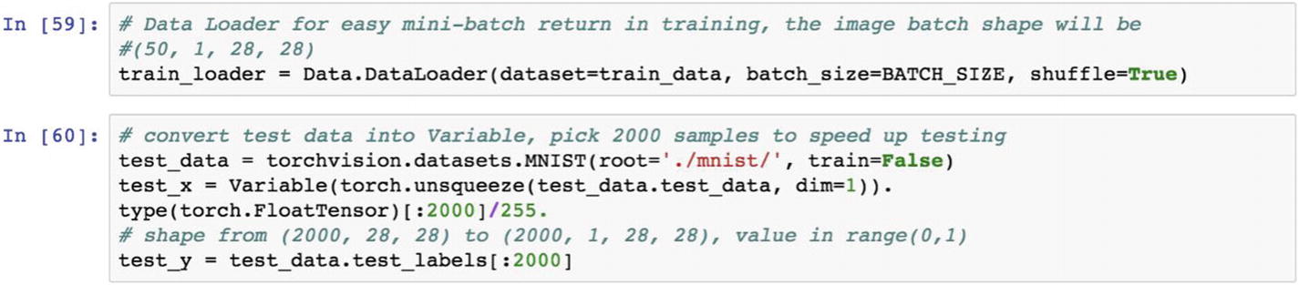
The preceding script shows what the sample image dataset would look like. To train the deep learning model, we need to convert the whole training dataset into mini batches, which help us with averaging the final accuracy of the model. By using the data loader function, we can load the training data and prepare the mini batches. The purpose of the shuffle selection in mini batches is to ensure that the model captures all the variations in the actual dataset.
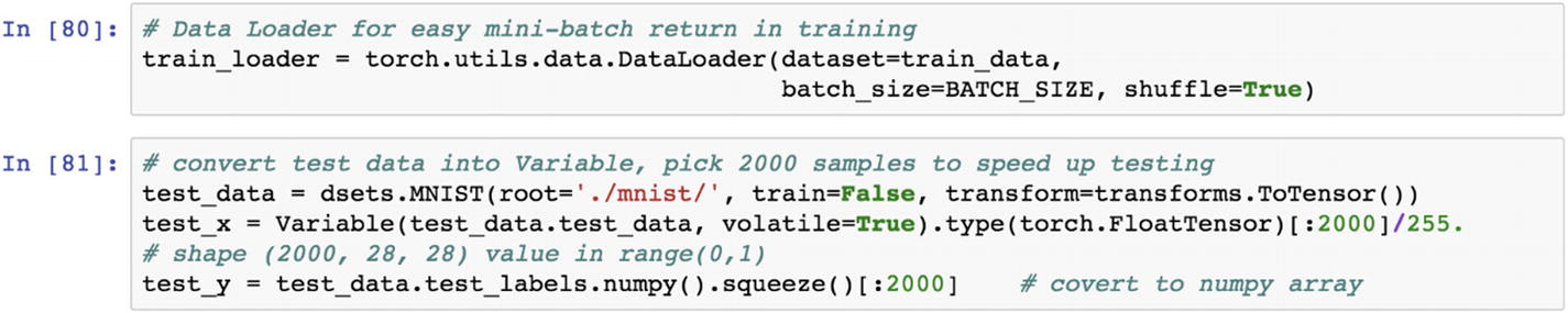
The preceding script prepares the training dataset. The test data is captured with the flag train=False. It is transformed to a tensor using the test data random sample of 2000 each at a time is picked up for testing the model. The test features set is converted to a variable format and the test label vector is represented in a NumPy array format.
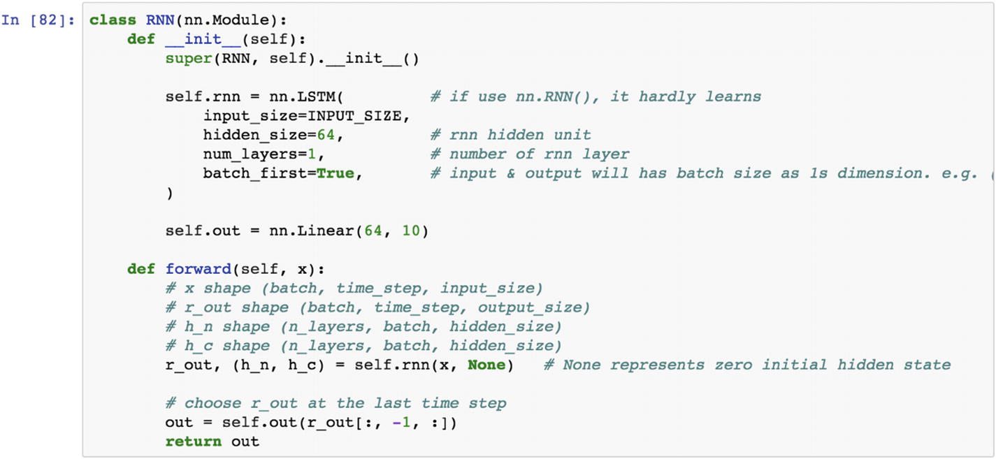
In the preceding RNN class, we are training an LSTM network , which is proven effective for holding memory for a long time, and thus helps in learning. If we use the nn.RNN() model, it hardly learns the parameters, because the vanilla implementation of RNN cannot hold or remember the information for a long period of time. In the LSTM network, the image width is considered the input size, hidden size is decided as the number of neurons in the hidden layer, num_layers shows the number of RNN layers in the network.
The RNN module, within the LSTM module, produces the output as a vector size of 64×10 because the output layer has digits to be classified as 0 to 9. The last forward function shows how to proceed with forward propagation in an RNN network.
The following script shows how the LSTM model is processed under the RNN class. In the LSTM function, we pass the input length as 28 and the number of neurons in the hidden layer as 64, and from the hidden 64 neurons to the output 10 neurons.
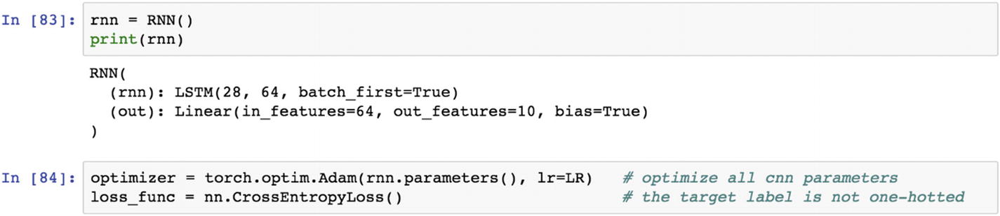
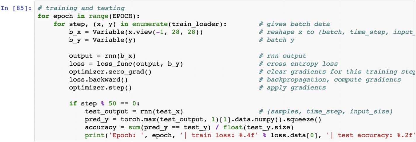
To optimize all RNN parameters, we use the Adam optimizer. Inside the function, we use the learning rate as well. The loss function used in this example is the cross-entropy loss function. We need to provide multiple epochs to get the best parameters.
In the following script, we are printing the training loss and the test accuracy. After one epoch, the test accuracy increases to 95% and the training loss reduces to 0.24.
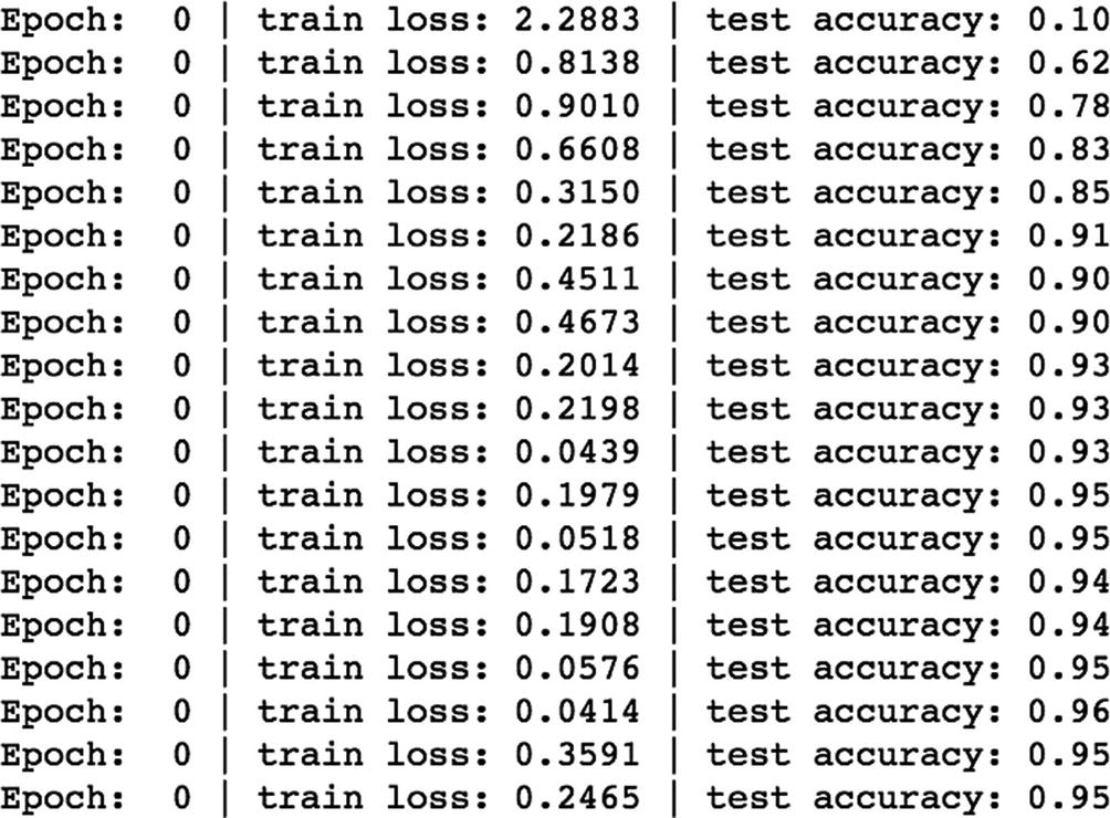
Once the model is trained, then the next step is to make predictions using the RNN model. Then we compare the actual vs. real output to assess how the model is performing.
Recipe 3-9. Implementing a RNN for Regression Problems
Problem
How do we set up a recurrent neural network for regression-based problems?
Solution
The regression model requires a target function and a feature set, and then a function to establish the relationship between the input and the output. In this example, we are going to use the recurrent neural network (RNN) for a regression task. Regression problems seem to be very simple; they do work best but are limited to data that shows clear linear relationships. They are quite complex when predicting nonlinear relationships between the input and the output.
How It Works
Let’s look at the following example that shows a nonlinear cyclical pattern between input and output data. In the previous recipe, we looked at an example of RNN in general for classification-related problems, where predicted the class of the input image. In regression, however, the architecture of RNN would change, because the objective is to predict the real valued output. The output layer would have one neuron in regression-related problems.
RNN time step implies that the last 10 values predict the current value, and the rolling happens after that.
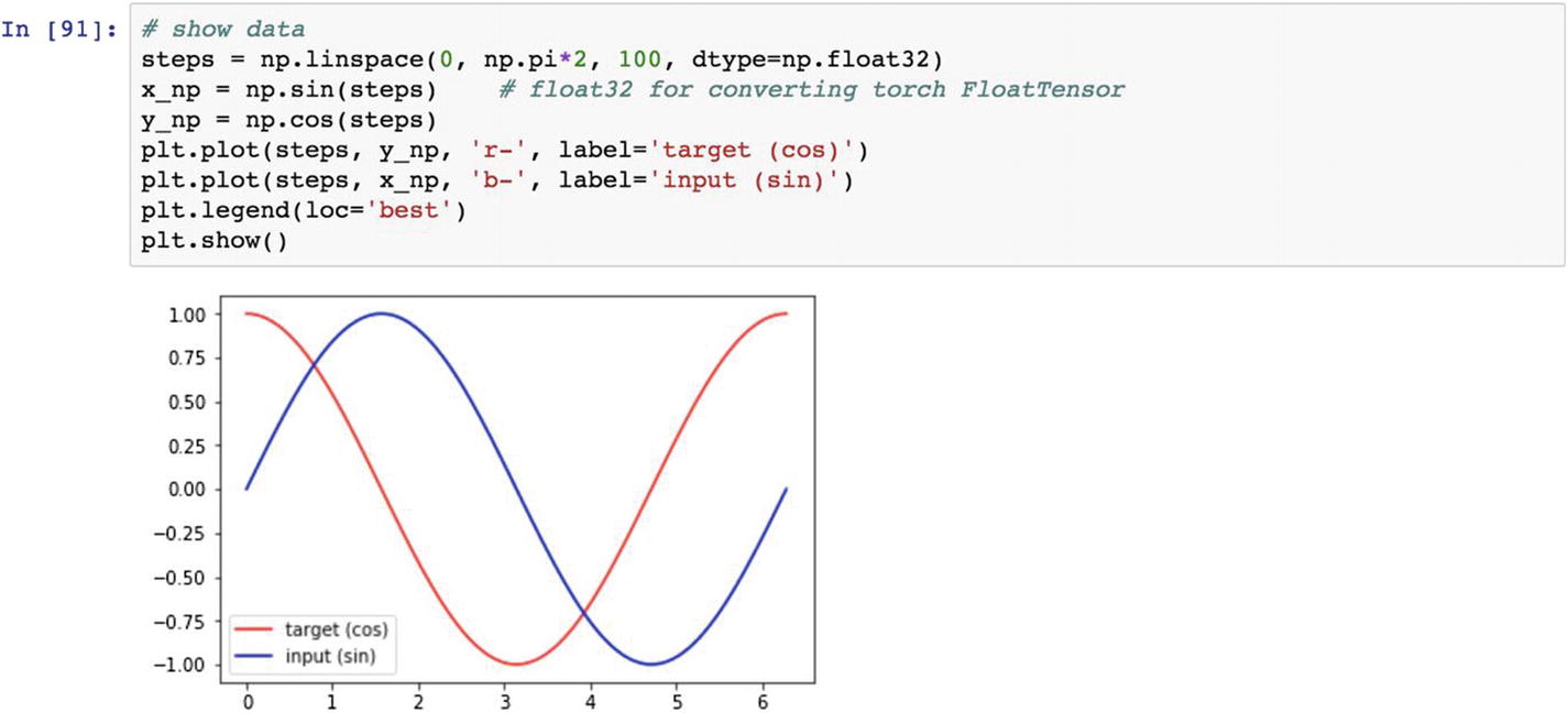
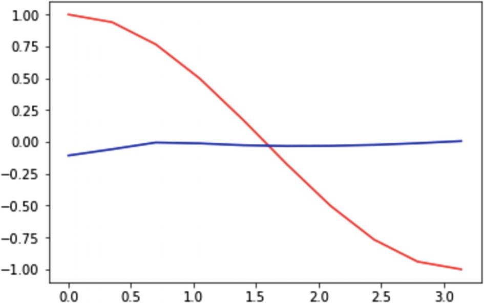
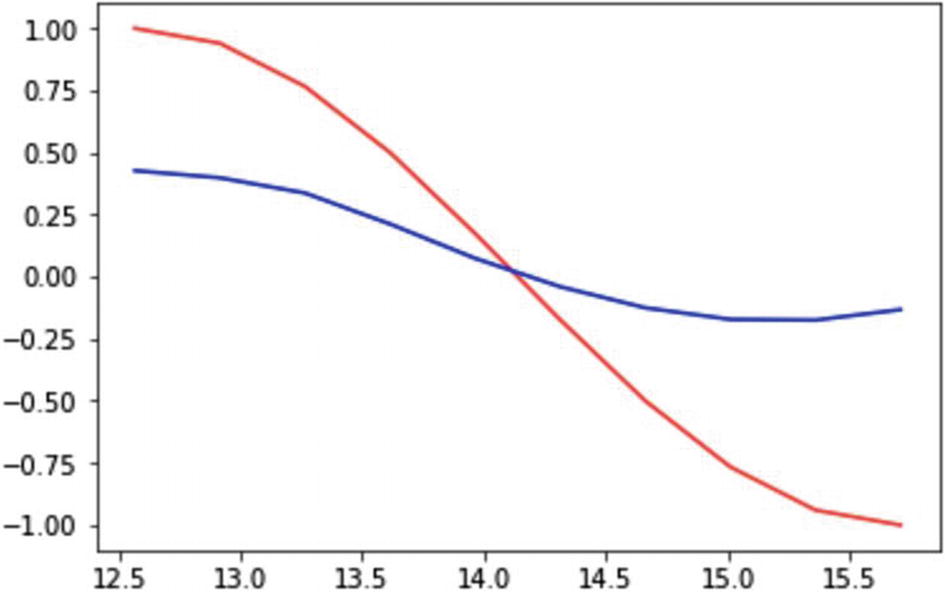
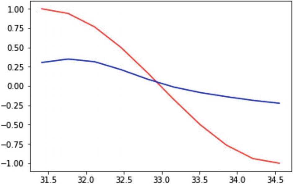
The following script shows some sample series in which the target cos function is approximated by the sin function.
Recipe 3-10. Using PyTorch Built-in Functions
Problem
How do we set up an RNN module and call the RNN function using PyTorch?
Solution
By using the built-in function available in the neural network module, we can implement an RNN model.
How It Works
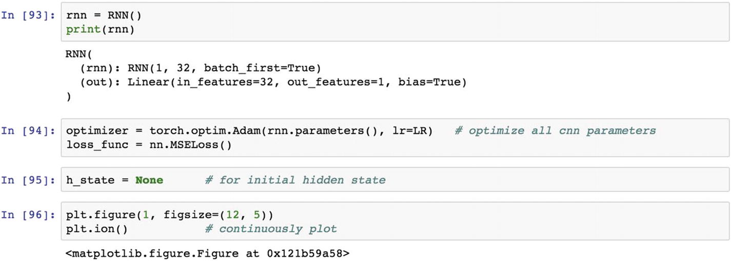
Let’s look at the following example. The neural network module in the PyTorch library contains the RNN function. In the following script, we use the input matrix size, the number of neurons in the hidden layer, and the number of hidden layers in the network.
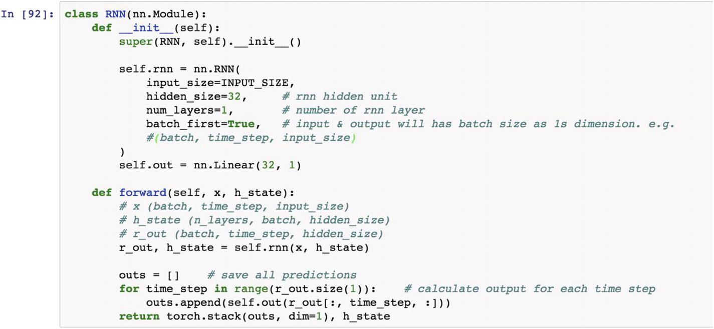
After creating the RNN class function, we need to provide the optimization function, which is Adam, and this time, the loss function is the mean square loss function. Since the objective is to make predictions of a continuous variable, we use MSELoss function in the optimization layer.
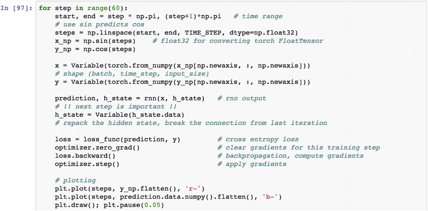
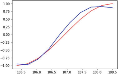
Now we iterate over 60 steps to predict the cos function generated from the sample space , and have it predicted by a sin function. The iterations take the learning rate defined as before, and backpropagate the error to reduce the MSE and improve the prediction.
Recipe 3-11. Working with Autoencoders
Problem
How do we perform clustering using the autoencoders function?
Solution
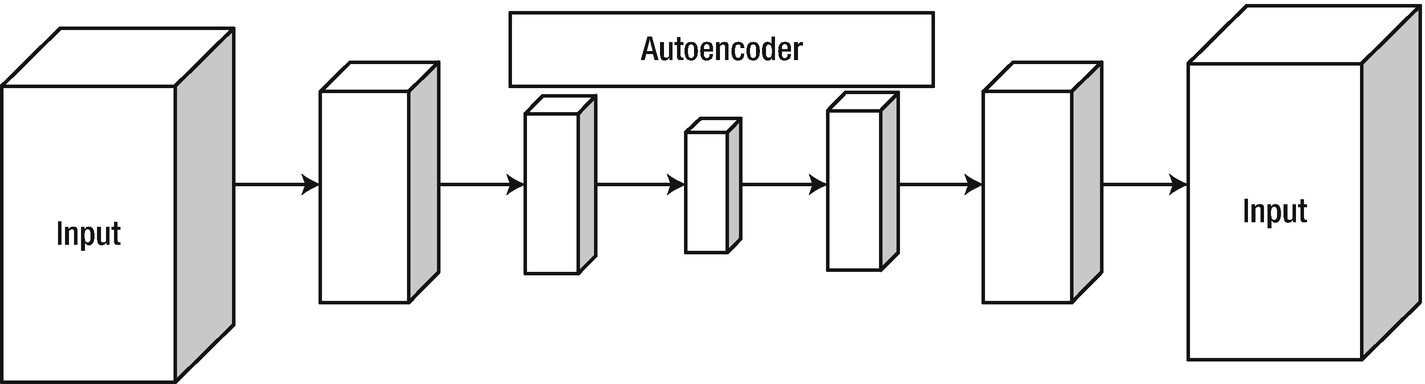
Autoencoder architecture
How It Works
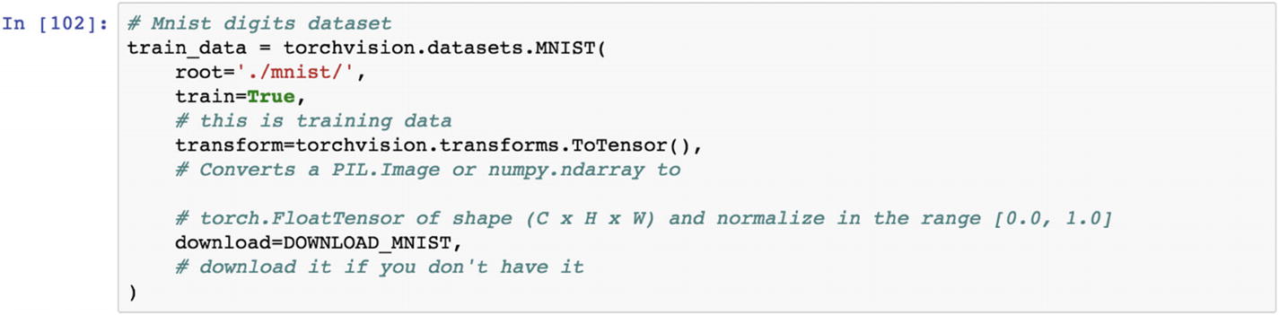
Let’s look at the following example. The torchvision library contains popular datasets, model architectures, and frameworks. Autoencoder is a process of identifying latent features from the dataset; it is used for classification, prediction, and clustering. If we put the input data in the input layer and the same dataset in the output layer, then we add multiple layers of hidden layers with many neurons, and then we pass through a series of epochs. We get a set of latent features in the innermost hidden layer. The weights or parameters in the central hidden layer are known as the autoencoder layer .
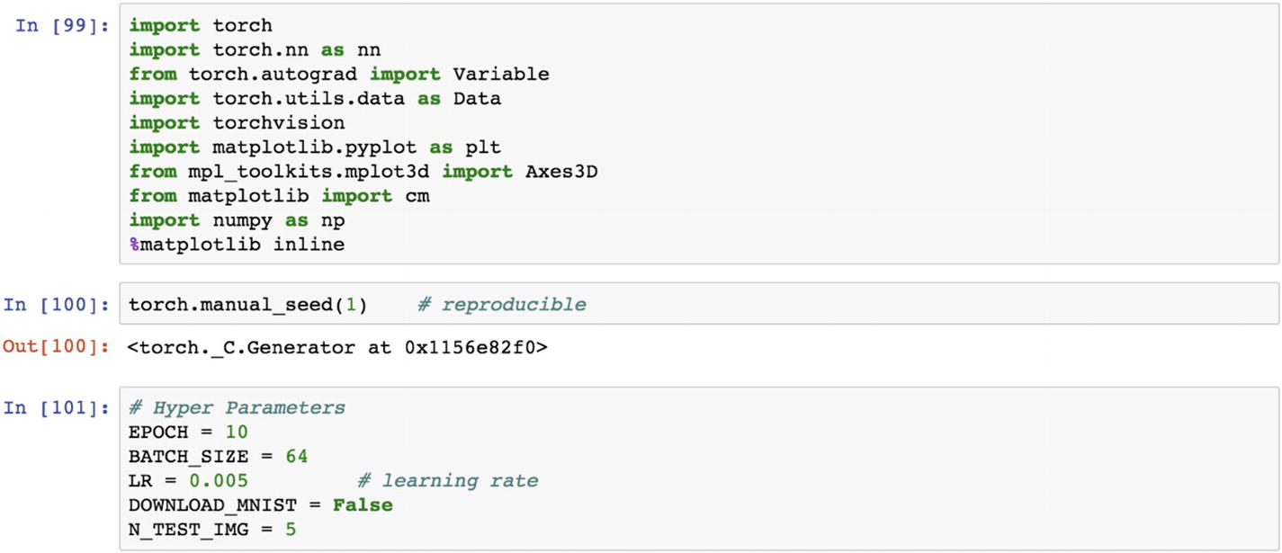
We again use the MNIST dataset to experiment with autoencoder functionality. This time we are taking 10 epochs, a batch size 64 to be passed to the network, a learning rate of 0.005, and 5 images for testing.
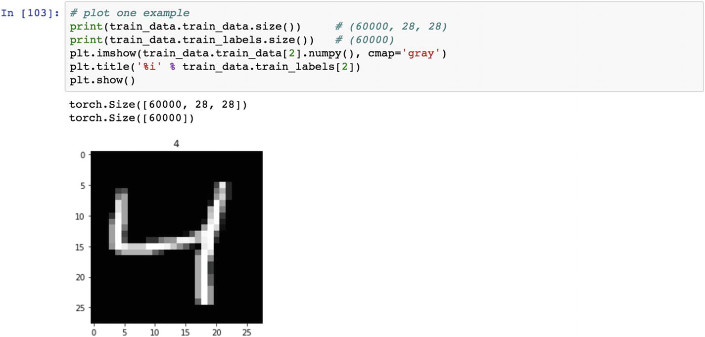
The following plot shows the dataset uploaded from the torchvision library and displayed as an image.
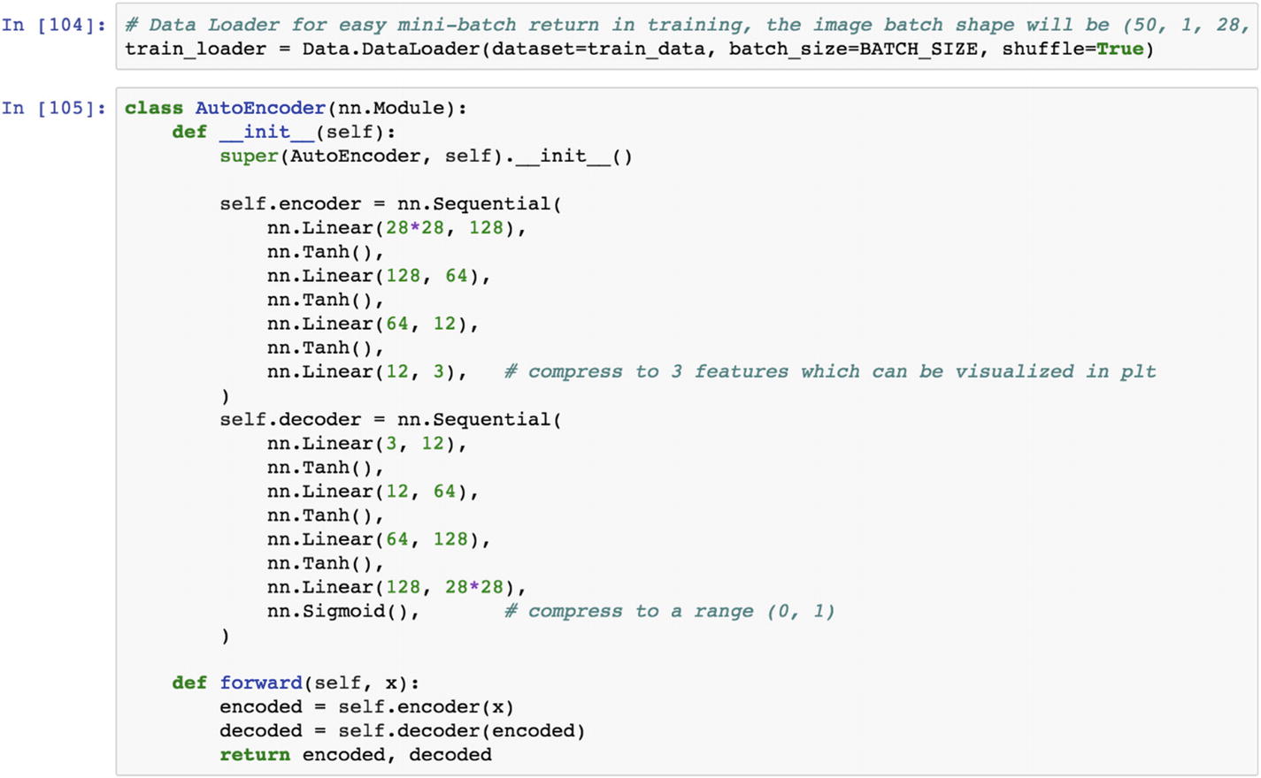
Let’s discuss the autoencoder architecture. The input has 784 features. It has a height of 28 and a width of 28. We pass the 784 neurons from the input layer to the first hidden layer, which has 128 neurons in it. Then we apply the hyperbolic tangent function to pass the information to the next hidden layer. The second hidden layer contains 128 input neurons and transforms it into 64 neurons. In the third hidden layer, we apply the hyperbolic tangent function to pass the information to the next hidden layer. The innermost layer contains three neurons, which are considered as three features, which is the end of the encoder layer. Then the decoder function expands the layer back to the 784 features in the output layer.
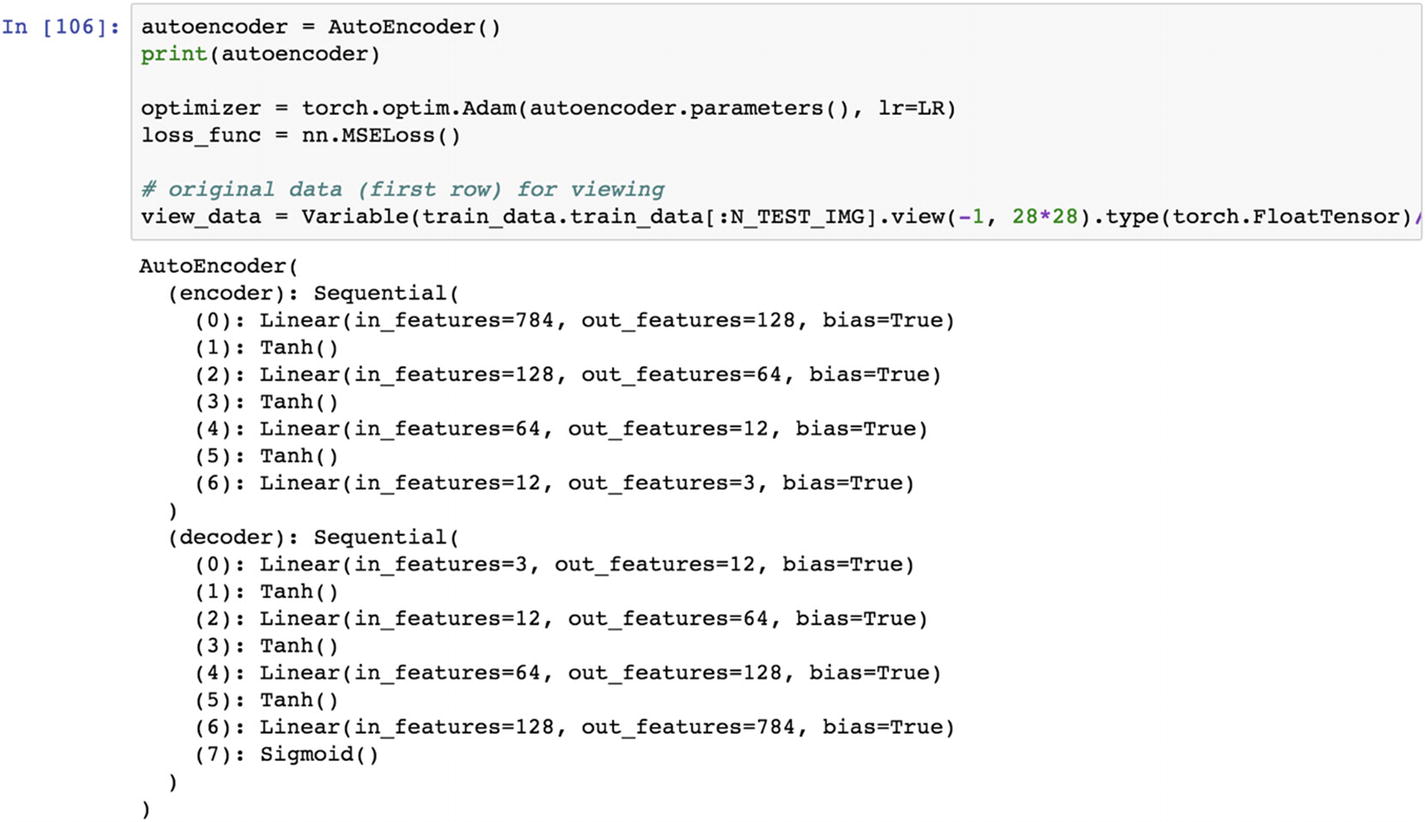
Once we set the architecture, then the normal process of making the loss function minimize corresponding to a learning rate and optimization function happens. The entire architecture passes through a series of epochs in order to reach the target output.
Recipe 3-12. Fine-Tuning Results Using Autoencoder
Problem
How do we set up iterations to fine-tune the results?
Solution
Conceptually, an autoencoder works the same as the clustering model. In unsupervised learning, the machine learns patterns from data and generalizes it to the new dataset. The learning happens by taking a set of input features. Autoencoder functions are also used for feature engineering.
How It Works
Let’s look at the following example. The same MNIST dataset is used as an example, and the objective is to understand the role of the epoch in achieving a better autoencoder layer. We increase the epoch size to reduce errors to a minimum; however, in practice, increasing the epoch has many challenges, including memory constraints.
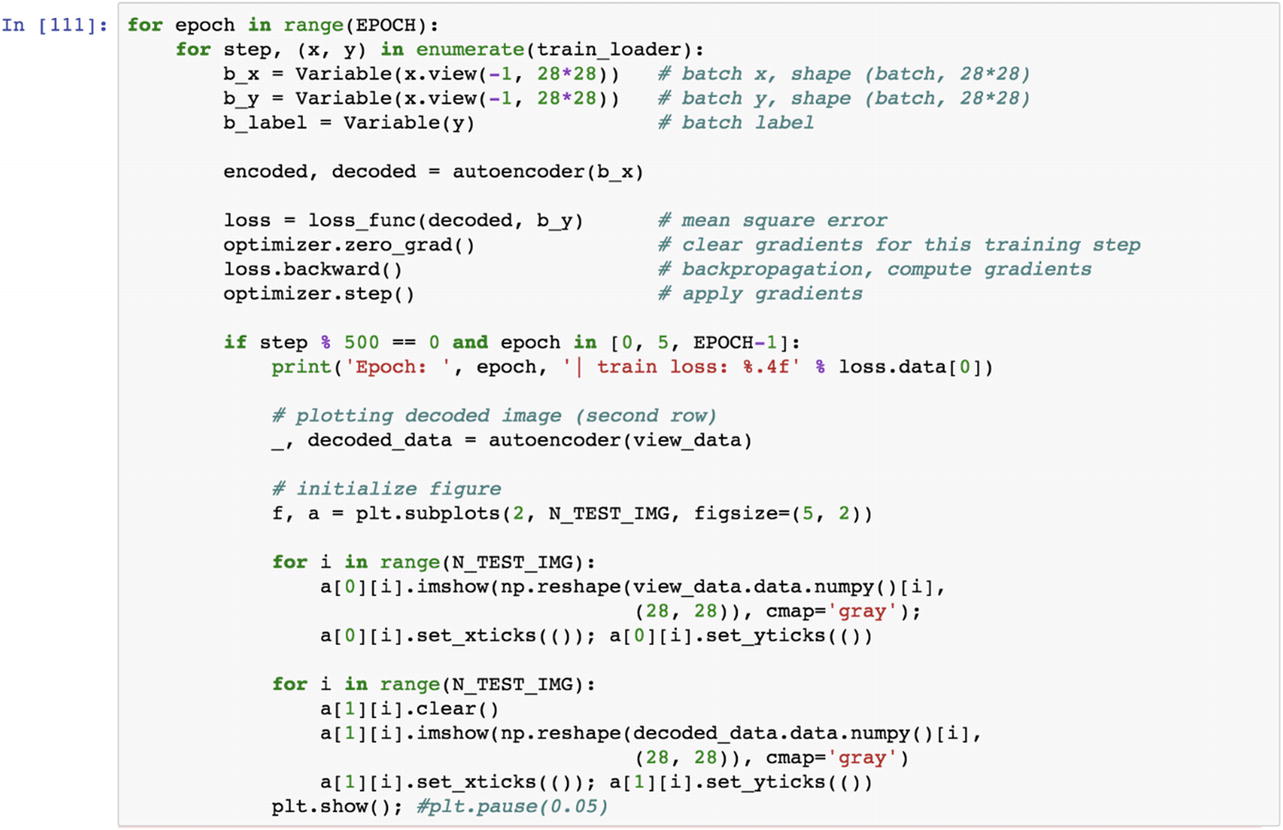
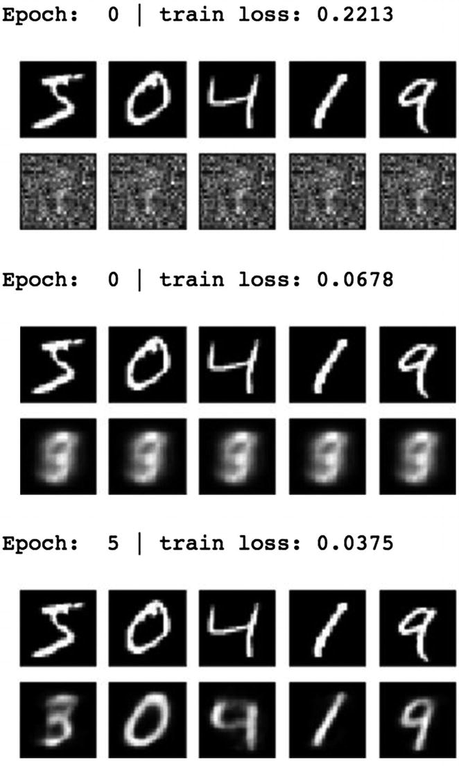
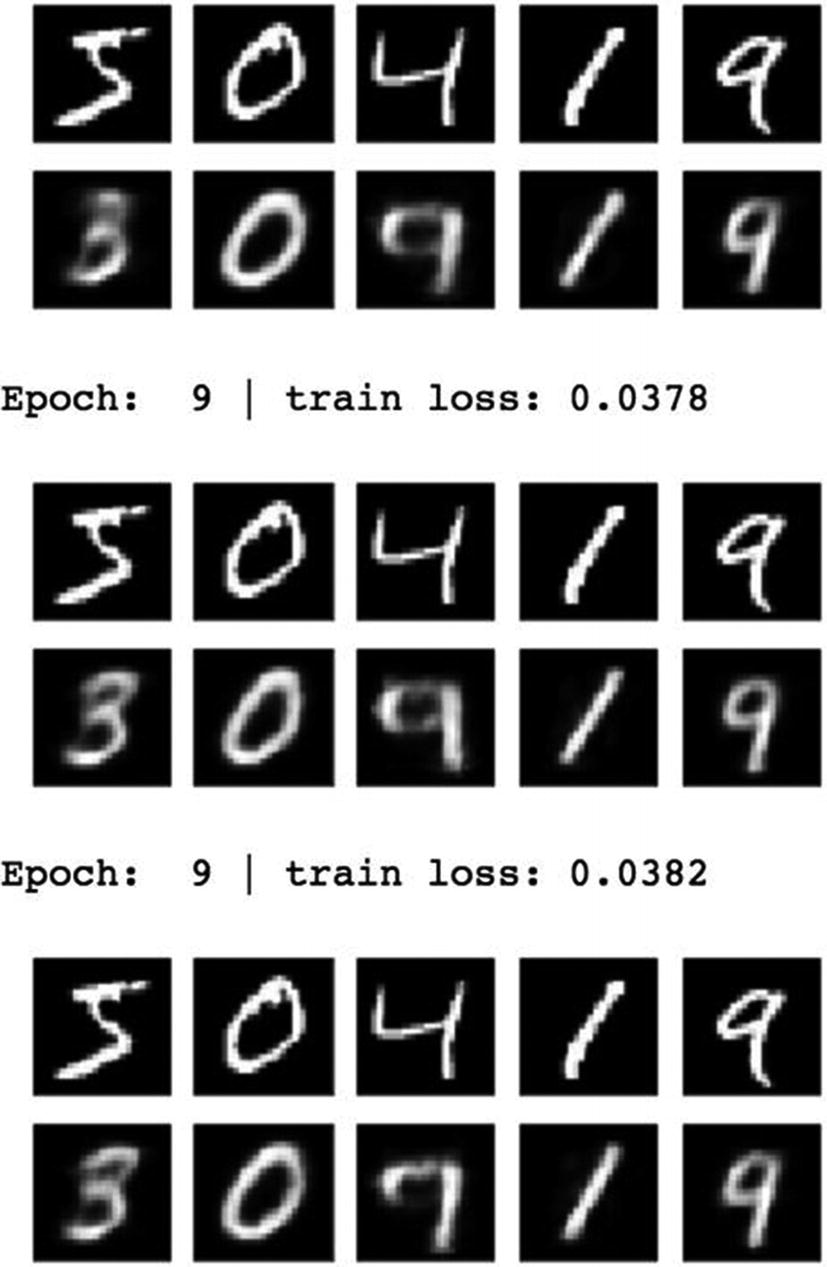
By using the encoder function, we can represent the input features into a set of latent features. By using the decoder function, however, we can reconstruct the image. Then we can match how image reconstruction is done by using the autoencoder functions. From the preceding set of graphs, it is clear that as we increase the epoch, the image recognition becomes transparent.
Recipe 3-13. Visualizing the Encoded Data in a 3D Plot
Problem
How do we visualize the MNIST data in a 3D plot?
Solution
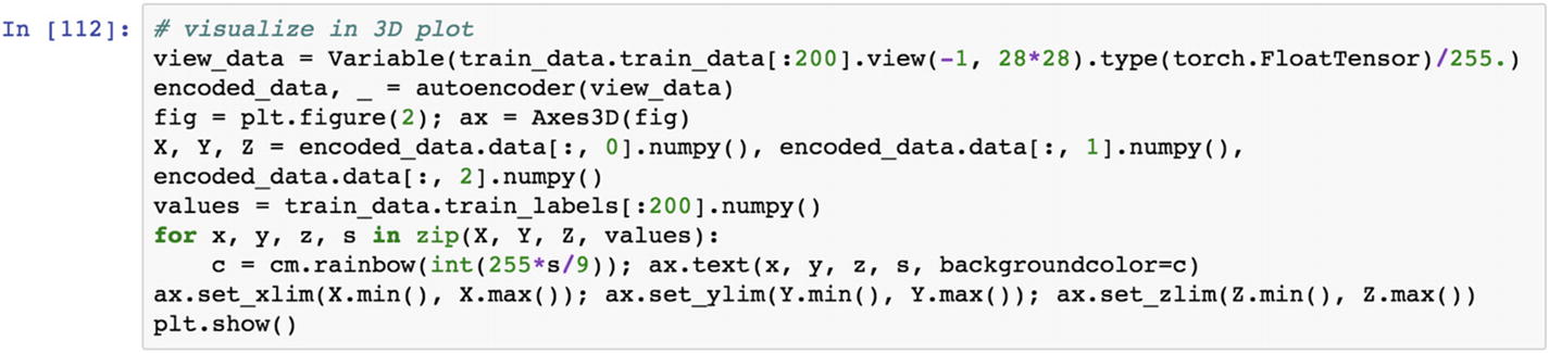
We use the autoencoder function to get the encoded features and then use the dataset to represent it in a 3D plane.
How It Works
Let’s look at the following example. This recipe is about how to represent the autoencoder function derived from the preceding recipe in the three-dimensional space, because we have three neurons in the innermost hidden layer. The following display shows a three-dimensional neuron.
Recipe 3-14. Restricting Model Overfitting
Problem
When we fit many neurons and layers to predict the target class or output variable, the function usually overfits the training dataset. Because of model overfitting, we cannot make a good prediction on the test set. The test accuracy is not the same as training accuracy. There would be deviations in training and test accuracy.
Solution
To restrict model overfitting, we consciously introduce dropout rate, which means randomly delete (let’s say) 10% or 20% of the weights in the network, and check the model accuracy at the same time. If we are able to match the same model accuracy after deleting the 10% or 20% of the weights, then our model is good.
How It Works
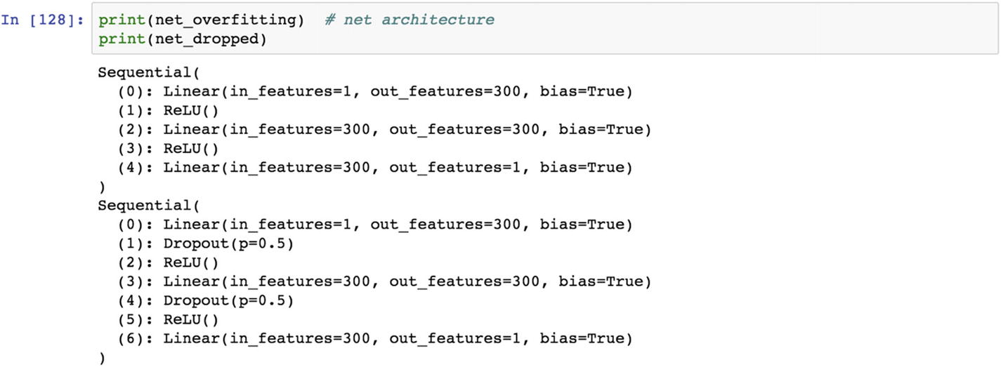
Let’s look at the following example. Model overfitting is occurs when the trained model does not generalize to other test case scenarios. It is identified when the training accuracy becomes significantly different from the test accuracy. To avoid model overfitting, we can introduce the dropout rate in the model.
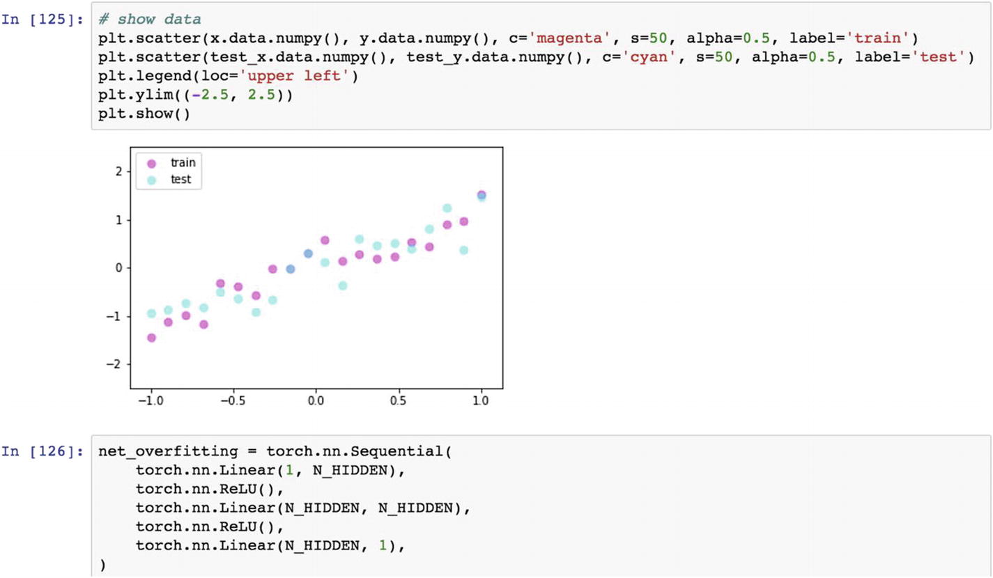
The dropout rate introduction to the hidden layer ensures that weights less than the threshold defined are removed from the architecture. A typical threshold for an application’s dropout rate is 20% to 50%. A 20% dropout rate implies a smaller degree of penalization; however, the 50% threshold implies heavy penalization of the model weights.
In the following script, we apply a 50% dropout rate to drop the weights from the model. We applied the dropout rate twice.
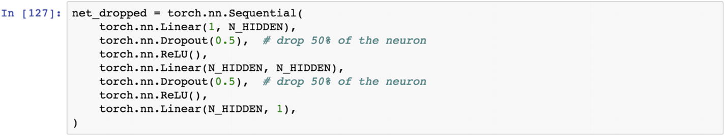

The selection of right dropout rate requires a fair idea about the business and domain.
Recipe 3-15. Visualizing the Model Overfit
Problem
Assess model overfitting.
Solution
We change the model hyperparameters and iteratively see if the model is overfitting data or not.
How It Works
Let’s look at the following example. The previous recipe covered two types of neural networks: overfitting and dropout rate. When the model parameters estimated from the data come closer to the actual data, for the training dataset and the same models differs from the test set, it is a clear sign of model overfit. To restrict model overfit, we can introduce the dropout rate, which deletes a certain percentage of connections (as in weights from the network) to allow the trained model to come to the real data.
In the following script, the iterations were taken 500 times. The predicted values are generated from the base model, which shows overfitting, and from the dropout model, which shows the deletion of some weights. In the same fashion, we create the two loss functions, backpropagation, and implementation of the optimizer.
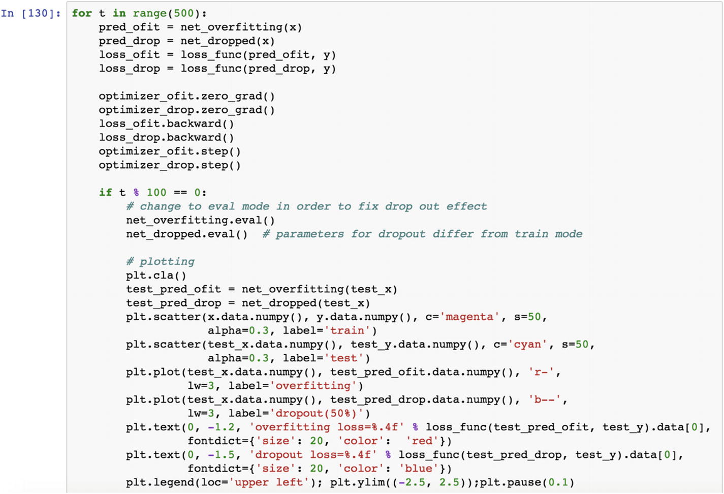
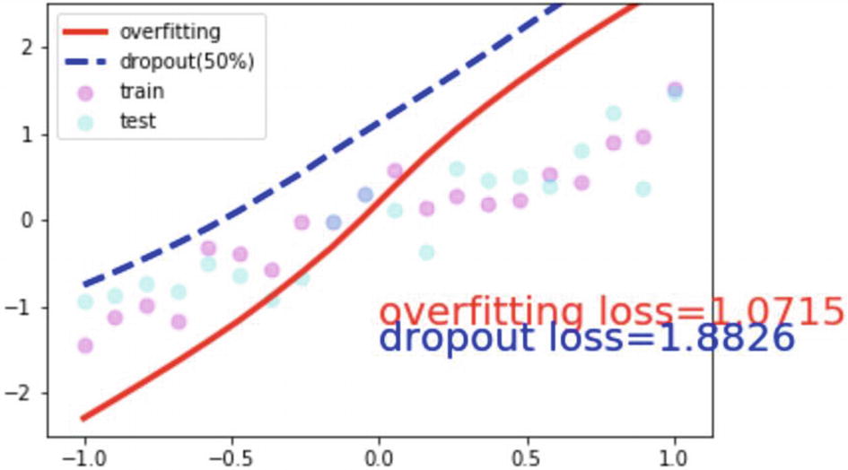
The initial round of plotting includes the overfitting loss and dropout loss and how it is different from the actual training and test data points from the preceding graph.
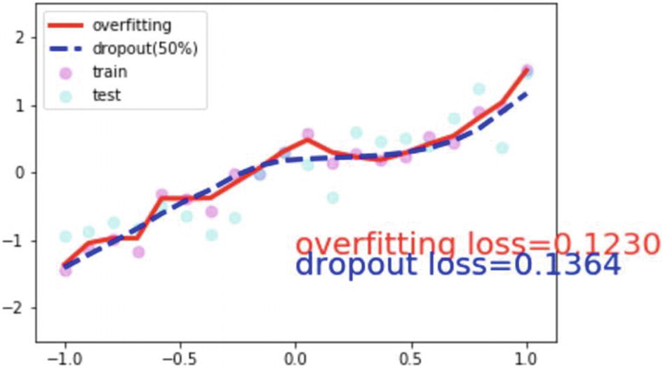
After many iterations, the preceding graph was generated by using the two functions with the actual model and with the dropout rate. The takeaway from this graph is that actual training data may get closer to the overfit model; however, the dropout model fits the data really well.
Recipe 3-16. Initializing Weights in the Dropout Rate
Problem
How do we delete the weights in a network? Should we delete randomly or by using any distribution?
Solution
We should delete the weights in the dropout layer based on probability distribution, rather than randomly.
How It Works
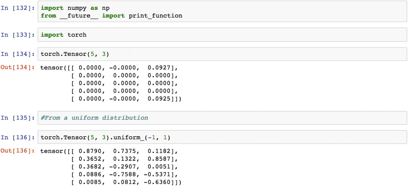
Let’s look at the following example. In the previous recipe, three layers of a dropout rate were introduced: one after the first hidden layer and two after the second hidden layer. The probability percentage was 0.50, which meant randomly delete 50% of the weights. Sometimes, random selection of weights from the network deletes relevant weights, so an alternative idea is to delete the weights in the network generated from statistical distribution.
The following script shows how to generate the weights from a uniform distribution, then we can use the set of weights in the network architecture.
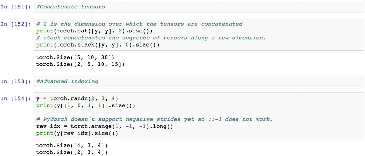
Recipe 3-17. Adding Math Operations
Problem
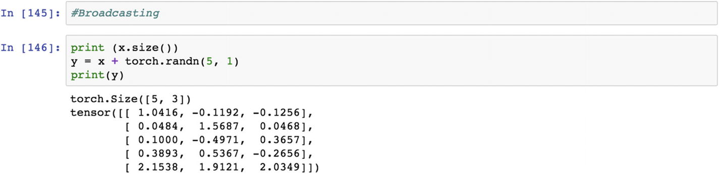
How do we set up the broadcasting function and optimize the convolution function?
Solution
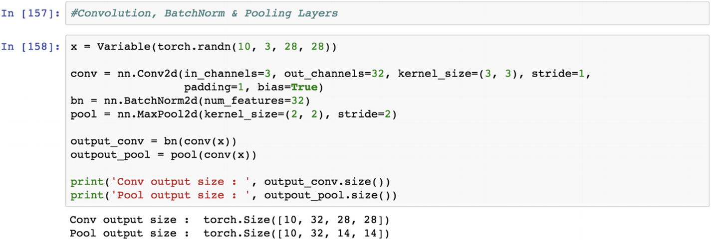
The script snippet shows how to introduce batch normalization when setting up a convolutional neural network model, and then further setting up a pooling layer.
How It Works
Let’s look at the following example. To introduce batch normalization in the convolutional layer of the neural network model, we need to perform tensor-based mathematical operations that are functionally different from other methods of computation.
The following piece of script shows how the batch normalization using a 2D layer is resolved before entering into the 2D max pooling layer.
Recipe 3-18. Embedding Layers in RNN
Problem
The recurrent neural network is used mostly for text processing. An embedded feature offers more accuracy on a standard RNN model than raw features. How do we create embedded features in an RNN?
Solution
The first step is to create an embedding layer, which is a fixed dictionary and fixed-size lookup table, and then introduce the dropout rate after than create gated recurrent unit.
How It Works
Let’s look at the following example. When textual data comes in as a sequence, the information is processed in a sequential way; for example, when we describe something, we use a set of words in sequence to convey the meaning. If we use the individual words as vectors to represent the data, the resulting dataset would be very sparse. But if we use a phrase-based approach or a combination of words to represent as feature vector, then the vectors become a dense layer. Dense vector layers are called word embeddings , as the embedding layer conveys a context or meaning as the result. It is definitely better than the bag-of-words approach.

Conclusion
This chapter covered using the PyTorch API, creating a simple neural network mode, and optimizing the parameters by changing the hyperparameters (i.e., learning rate, epochs, gradients drop). We looked at recipes on how to create a convolutional neural network and a recurrent neural network, and introduced the dropout rate in these networks to control model overfitting.
We took small tensors to follow what exactly goes on behind the scenes with calculations and so forth. We only need to define the problem statement, create features, and apply the recipe to get results. In the next chapter, we implement many more examples with PyTorch.