Problem

What are the activation functions and how do they work in real projects? How do you implement an activation function using PyTorch?

Solution

Activation function is a mathematical formula that transforms a vector available in a binary, float, or integer format to another format based on the type of mathematical transformation function. The neurons are present in different layers—input, hidden, and output, which are interconnected through a mathematical function called an activation function. There are different variants of activation functions, which are explained next. Understanding the activation function helps in accurately implementing a neural network model.

How It Works

All the activation functions that are part of a neural network model can be broadly classified as linear functions and nonlinear functions. The PyTorch torch.nn module creates any type of a neural network model. Let’s look at some examples of the deployment of activation functions using PyTorch and the torch.nn module.

The core differences between PyTorch and TensorFlow is the way a computational graph is defined, the way the two frameworks perform calculations, and the amount of flexibility we have in changing the script and introducing other Python-based libraries in it. In TensorFlow, we need to define the variables and placeholders before we initialize the model. We also need to keep track of objects that we need later, and for that we need a placeholder. In TensorFlow, we need to define the model first, and then compile and run; however, in PyTorch, we can define the model as we go—we don’t have to keep placeholders in the code. That’s why the PyTorch framework is dynamic.

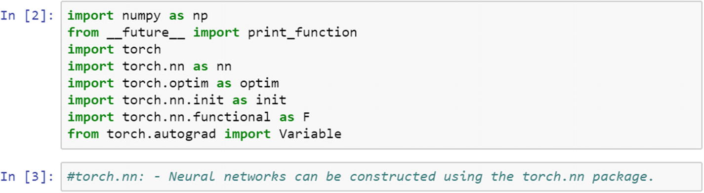
Linear Function

A linear function is a simple functions typically used to transfer information from the demapping layer to the output layer. We use the linear function in places where variations in data are lower. In a deep learning model, practitioners typically use a linear function in the last hidden layer to the output layer. In the linear function, the output is always confined to a specific range; because of that, it is used in the last hidden layer in a deep learning model, or in linear regression–based tasks, or in a deep learning model where the task is to predict the outcome from the input dataset. The following is the formula.

Bilinear Function

A bilinear function is a simple functions typically used to transfer information. It applies a bilinear transformation to incoming data.

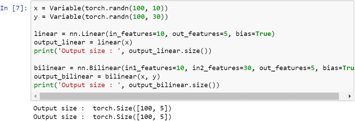
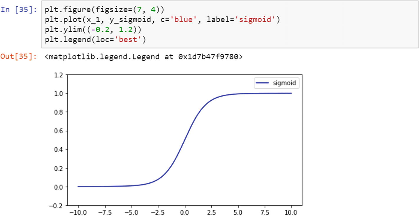
Sigmoid Function

A sigmoid function is frequently used by professionals in data mining and analytics because it is easier to explain and implement. It is a nonlinear function. When we pass weights from the input layer to the hidden layer in a neural network, we want our model to capture all sorts of nonlinearity present in the data; hence, using the sigmoid function in the hidden layers of a neural network is recommended. The nonlinear functions help with generalizing the dataset. It is easier to compute the gradient of a function using a nonlinear function.

The sigmoid function is a specific nonlinear activation function. The sigmoid function output is always confined within 0 and 1; therefore, it is mostly used in performing classification-based tasks. One of the limitations of the sigmoid function is that it may get stuck in local minima. An advantage is that it provides probability of belonging to the class. The following is its equation.

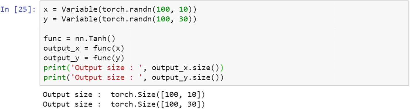
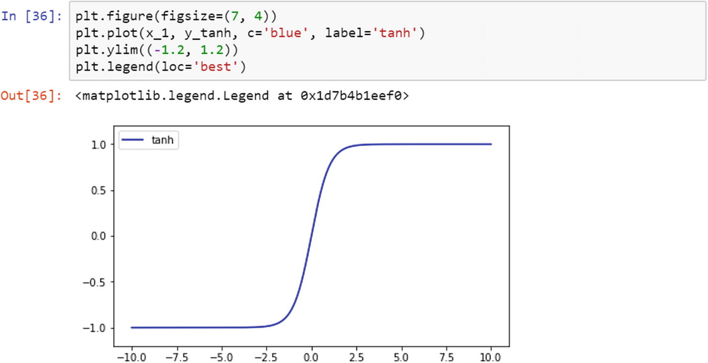
Hyperbolic Tangent Function

A hyperbolic tangent function is another variant of a transformation function. It is used to transform information from the mapping layer to the hidden layer. It is typically used between the hidden layers of a neural network model. The range of the tanh function is between –1 and +1.

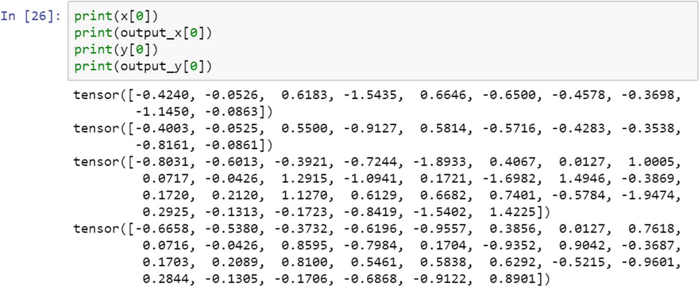
Log Sigmoid Transfer Function

The following formula explains the log sigmoid transfer function, which is used in mapping the input layer to the hidden layer. If the data is not binary, and it is a float type with a lot of outliers (as in large numeric values present in the input feature), then we should use the log sigmoid transfer function.

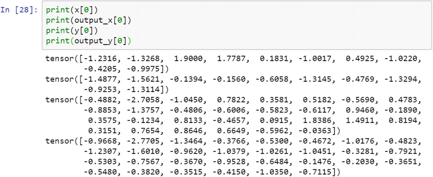
ReLU Function

The rectified linear unit (ReLu) is another activation function. It is used in transferring information from the input layer to the output layer. ReLu is mostly used in a convolutional neural network model. The range in which this activation function operates is from 0 to infinity. It is mostly used between different hidden layers in a neural network model.

The different types of transfer functions are interchangeable in a neural network architecture. They can be used in different stages , such as the input to the hidden layer, the hidden layer to the output layer, and so forth, to improve the model’s accuracy.

Leaky ReLU

In a standard neural network model, a dying gradient problem is common. To avoid this issue, leaky ReLU is applied. Leaky ReLU allows a small and non-zero gradient when the unit is not active.

Problem

How do we visualize the activation functions? The visualization of activation functions is important in correctly building a neural network model.

Solution

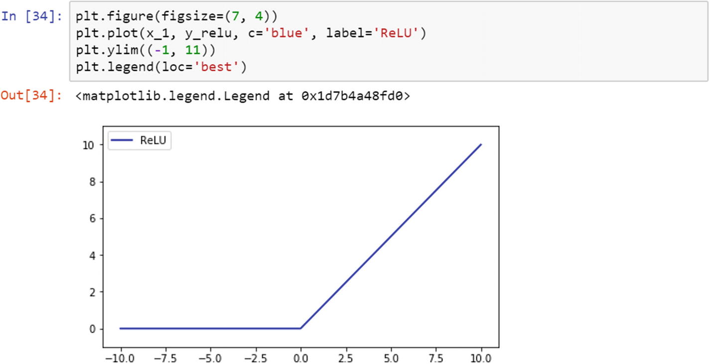
The activation functions translate the data from one layer into another layer. The transformed data can be plotted against the actual tensor to visualize the function. We have taken a sample tensor, converted it to a PyTorch variable, applied the function, and stored it as another tensor. Represent the actual tensor and the transformed tensor using matplotlib.

How It Works

The right choice of an activation function will not only provide better accuracy but also help with extracting meaningful information.

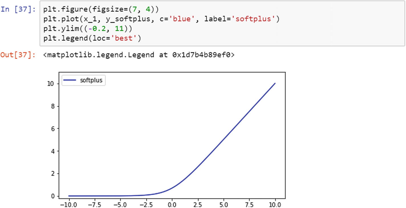
In this script, we have an array in the linear space between –10 and +10, and we have 1500 sample points. We converted the vector to a Torch variable, and then made a copy as a NumPy variable for plotting the graph. Then, we calculated the activation functions. The following images show the activation functions.

Problem

How do we build a basic neural network model using PyTorch?

Solution

A basic neural network model in PyTorch requires six steps: preparing training data, initializing weights, creating a basic network model, calculating the loss function, selecting the learning rate, and optimizing the loss function with respect to the model’s parameters.

How It Works

Let’s follow a step-by-step approach to create a basic neural network model.

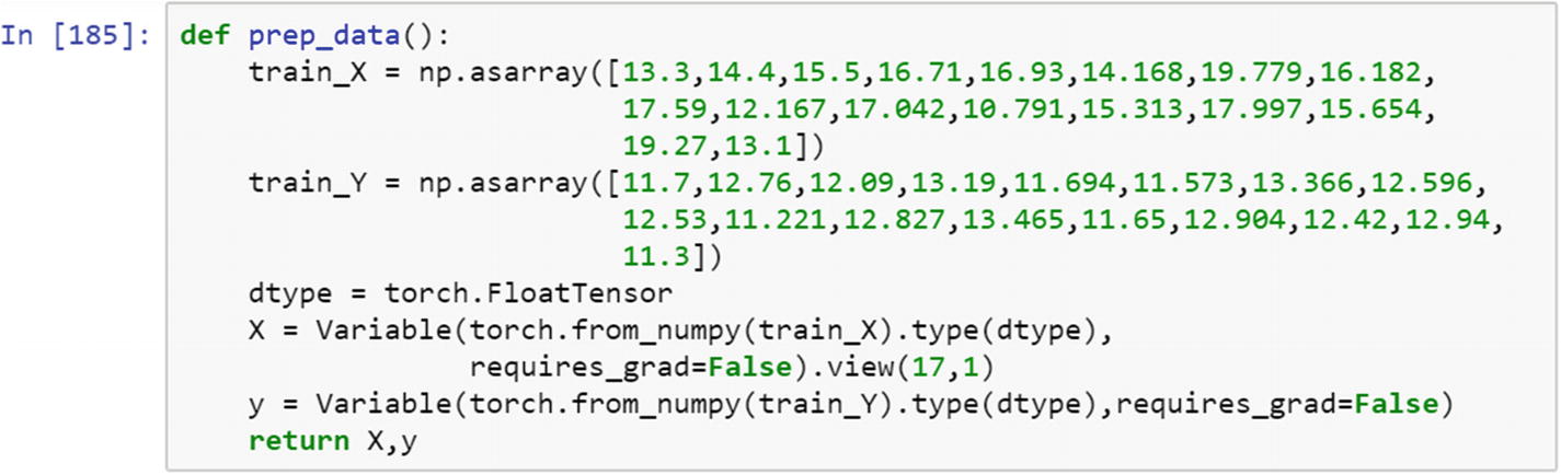
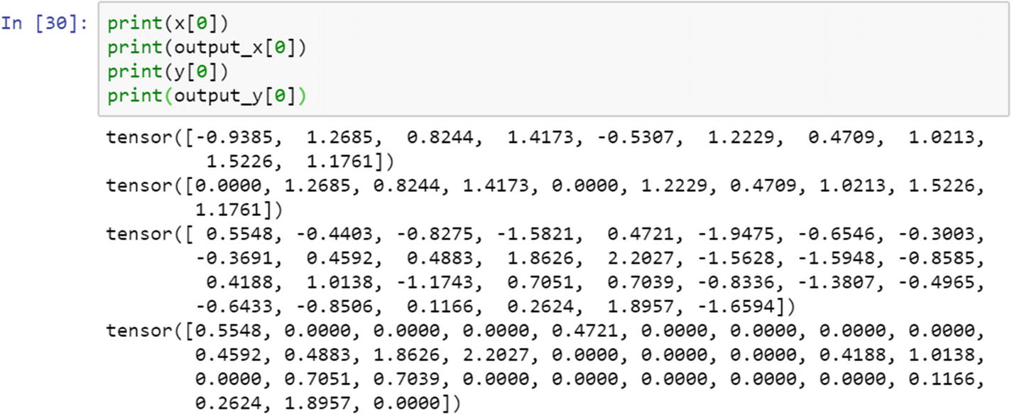
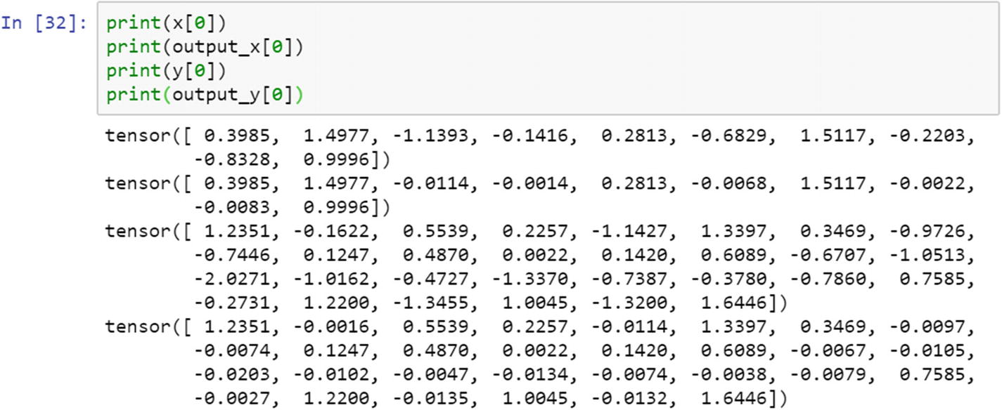
To show a sample neural network model, we prepare the dataset and change the data type to a float tensor. When we work on a project, data preparation for building it is a separate activity. Data preparation should be done in the proper way. In the preceding step, train x and train y are two NumPy vectors. Next, we change the data type to a float tensor because it is necessary for matrix multiplication. The next step is to convert it to variable, because a variable has three properties that help us fine-tune the object. In the dataset, we have 17 data points on one dimension.

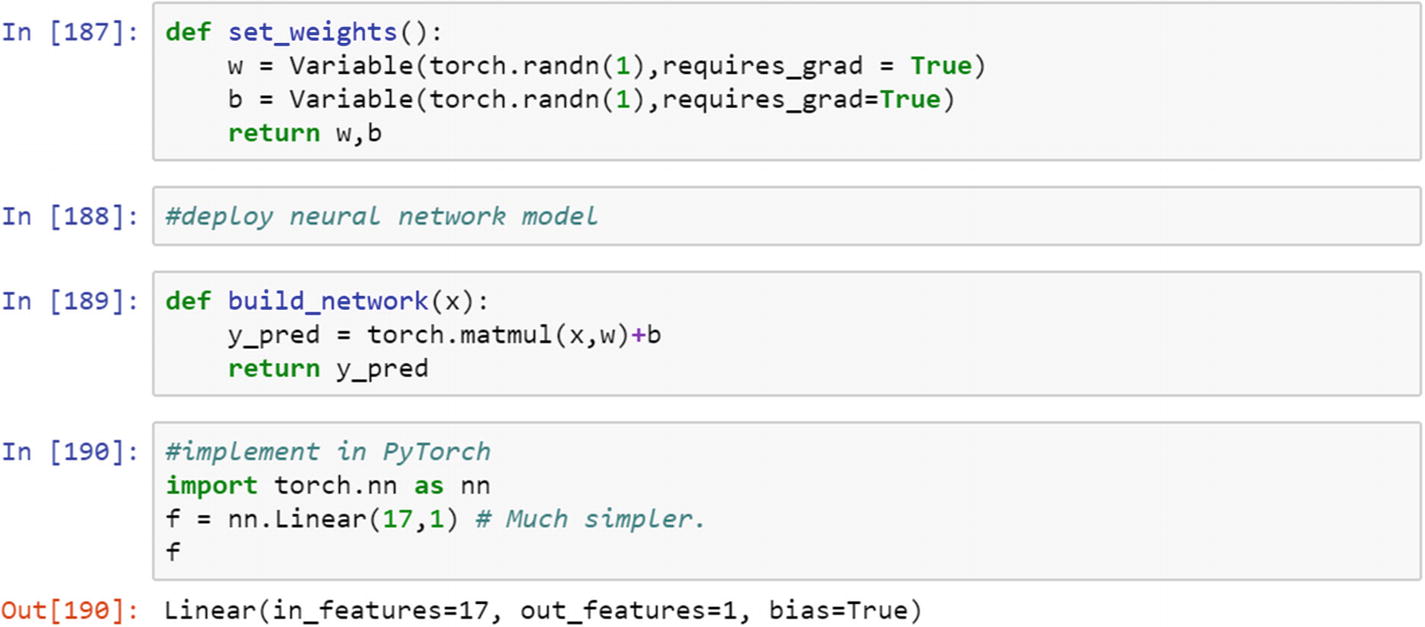
The set_weight() function initializes the random weights that the neural network model will use in forward propagation. We need two tensors weights and biases. The build_network() function simply multiplies the weights with input, adds the bias to it, and generates the predicted values. This is a custom function that we built. If we need to implement the same thing in PyTorch, then it is much simpler to use nn.Linear() when we need to use it for linear regression.

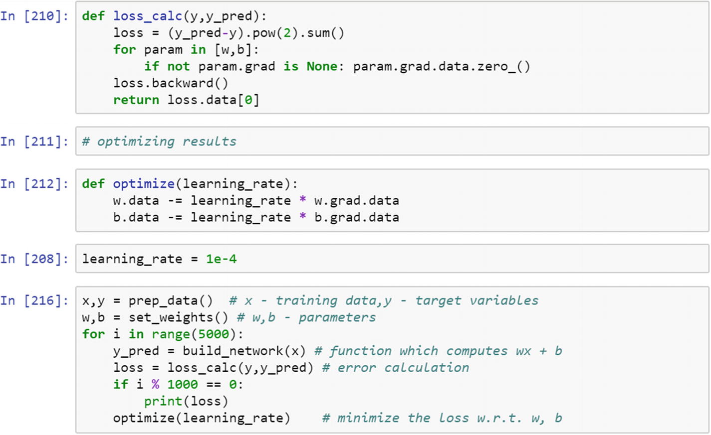
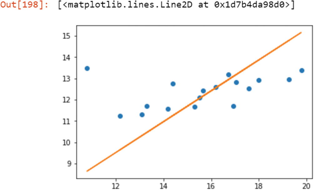
Once we define a network structure, then we need to compare the results with the output to assess the prediction step. The metric that tracks the accuracy of the system is the loss function, which we want to be minimal. The loss function may have a different shape. How do we know exactly where the loss is at a minimum, which corresponds to which iteration is providing the best results? To know this, we need to apply the optimization function on the loss function; it finds the minimum loss value. Then we can extract the parameters corresponding to that iteration.

Median, mode and standard deviation computation can be written in the sa

Standard deviation shows the deviation from the measures of central tendency, which indicates the consistency of the data/variable. It shows whether there is enough fluctuation in data or not.

Problem

What is tensor differentiation, and how is it relevant in computational graph execution using the PyTorch framework?

Solution

The computational graph network is represented by nodes and connected through functions. There are two different kinds of nodes: dependent and independent. Dependent nodes are waiting for results from other nodes to process the input. Independent nodes are connected and are either constants or the results. Tensor differentiation is an efficient method to perform computation in a computational graph environment.

How It Works

In a computational graph, tensor differentiation is very effective because the tensors can be computed as parallel nodes, multiprocess nodes, or multithreading nodes. The major deep learning and neural computation frameworks include this tensor differentiation.

Autograd is the function that helps perform tensor differentiation, which means calculating the gradients or slope of the error function, and backpropagating errors through the neural network to fine-tune the weights and biases. Through the learning rate and iteration, it tries to reduce the error value or loss function.

To apply tensor differentiation, the nn.backward() method needs to be applied. Let’s take an example and see how the error gradients are backpropagated. To update the curve of the loss function, or to find where the shape of the loss function is minimum and in which direction it is moving, a derivative calculation is required. Tensor differentiation is a way to compute the slope of the function in a computational graph.

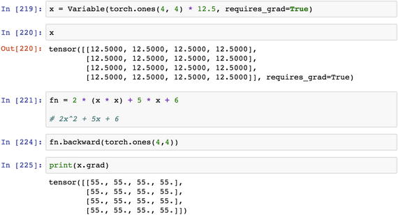
In this script, the x is a sample tensor , for which automatic gradient calculation needs to happen. The fn is a linear function that is created using the x variable. Using the backward function, we can perform a backpropagation calculation. The .grad() function holds the final output from the tensor differentiation.