© B.J. Korites 2018
B.J. KoritesPython Graphicshttps://doi.org/10.1007/978-1-4842-3378-8_6

6. Hidden Line Removal

B. J. Korites1 
(1)
Duxbury, Massachusetts, USA
 

Most of the models used in the previous chapters were essentially stick figures constructed of dots and lines. When such objects are viewed in three dimensions, it is possible to see the lines on the back side, as if the objects were transparent. This chapter is concerned with removing the lines, which would normally be hidden, from objects so they appear solid.

This chapter will cover two types of situations. The first is called intra-object hidden line removal. This refers to removing hidden lines from a single object. We assume that most objects are constructed of flat planes; the examples are a box, a pyramid, and a spherical surface that is approximated by planes. The technique you will use relies on determining whether a particular plane faces toward the viewer, in which case it is visible and is plotted, or away from the viewer, in which case it is not visible and is not plotted.

Inter-object hidden line removal, on the other hand, refers to a system of more than one object, such as two planes, one behind the other. Here the general approach is to use some of the ray tracing techniques that were developed in the previous chapter to find intersections between lines and surfaces. You start by drawing the back object using dots or short line segments. At each point you construct a line (ray) going toward the observer, who is in the -z direction, and see if it intersects with the front object. If it does, that point on the back object is hidden and is not plotted.

6.1 Box

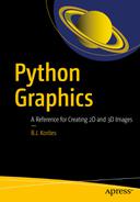
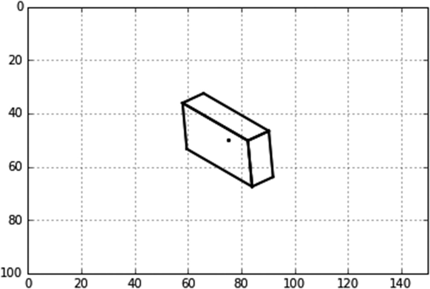
As an example of intra-object hidden line removal, let’s start off with a simple box, as shown in Figures 6-1 and 6-2. They were drawn by Listing 6-1. Figures 6-3, 6-4, and 6-5 show the model used by the program.

In Figure 6-3, you see that the box has eight corners, numbered 0 to 7. At corner 0, there are two vectors: V01, which goes from corner 0 to 1, and V03, which goes from 0 to 3. Looking at the 0,1,2,3 face first, as the box is rotated, the strategy is to determine if it is tilted toward or away from an observer who is in the -z direction. If it is facing toward the observer, the edges of the face are plotted. If it is facing away from the observer, they are not plotted. How do you determine if the face is facing the observer? The cross (vector) product V03×V01 gives a vector N, which is normal to the 0,1,2,3 face, so
$$ mathbf{V}mathbf{03}=V03xwidehat{mathbf{i}}+V03ywidehat{mathbf{j}}+V03zwidehat{mathbf{k}} $$
(6-1)
$$ mathbf{V}mathbf{01}=V01xwidehat{mathbf{i}}+V01ywidehat{mathbf{j}}+V01zwidehat{mathbf{k}} $$
(6-2)
$$ V03x=xleft[3
ight]-xleft[0
ight] $$
(6-3)
$$ V03y=yleft[3
ight]-yleft[0
ight] $$
(6-4)
$$ V03z=zleft[3
ight]-zleft[0
ight] $$
(6-5)
$$ V01x=xleft[1
ight]-xleft[0
ight] $$
(6-6)
$$ V01y=yleft[1
ight]-yleft[0
ight] $$
(6-7)
$$ V01z=zleft[1
ight]-zleft[0
ight] $$
(6-8)
$$ mathbf{N}=mathbf{V}mathbf{03}	imes mathbf{V}mathbf{01}=left[egin{array}{ccc}widehat{mathbf{i}}& widehat{mathbf{j}}& widehat{mathbf{k}}\ {}V03x& V03y& V03z\ {}V01x& V01y& V01zend{array}
ight] $$
(6-9)
$$ mathbf{N}= Nxwidehat{mathbf{i}}+ Nywidehat{mathbf{j}}+ Nzwidehat{mathbf{k}} $$
(6-10)
$$ {displaystyle egin{array}{l}mathrm{N}=widehat{mathbf{i}}kern0.125em left[V03ycdotp V01z-V03zcdotp V01y
ight]+widehat{mathbf{j}}kern0.125em left[V03zcdotp V01x-V03xcdotp V01z
ight]\ {}kern18em +widehat{mathbf{k}}underset{Nz}{underbrace{left[V03xcdotp V01y-V03ycdotp V01x
ight]}}end{array}} $$
(6-11)

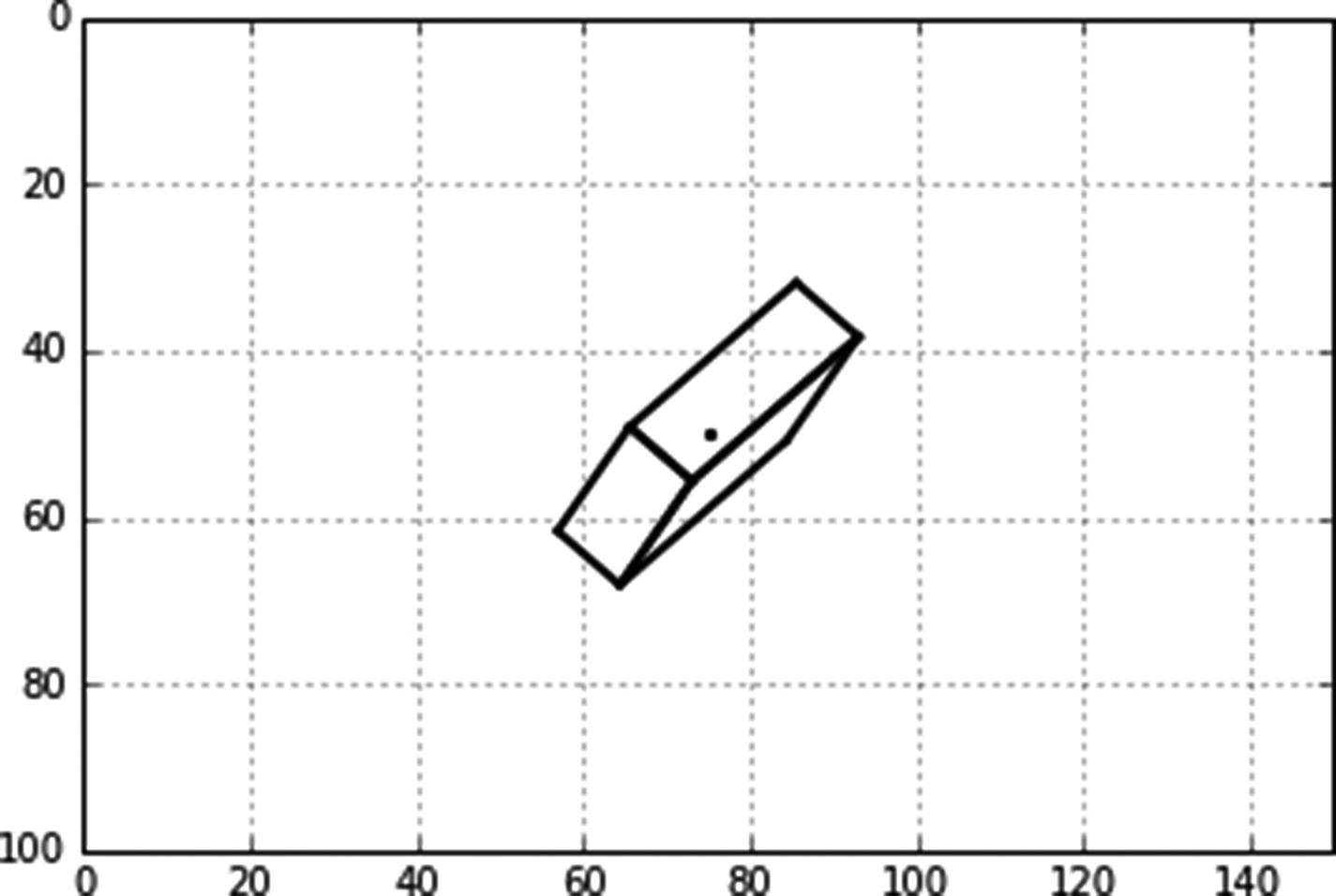
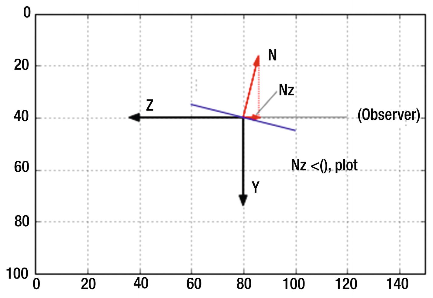
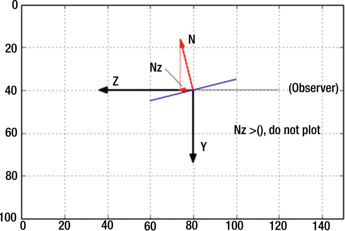
You can determine if the plane is facing toward or away from the observer by the value of Nz, N’s z component. Figures 6-4 and 6-5 show a plane (blue) relative to an observer. This is the side view of one of the faces of the box shown in Figure 6-3. The observer is on the right side of the coordinate system looking in the +z direction. Referring to Figure 6-4, if the z component of N, Nz in Equation 6-11, is < 0 (i.e. pointing in the -z direction), the plane is facing the observer, it is visible to the observer, and it is plotted. If Nz is positive (i.e. pointing in the +z direction), as shown in Figure 6-5, the face is tilted away from the observer, in which case it is not seen by the observer and is not plotted. Note that you can use the full vector V rather than a unit vector since you are only concerned with the sign of V.

What about the other faces? The 4,5,6,7 face is parallel to 0,1,2,3 so its outward pointing normal vector is opposite to that of face 0,1,2,3. You do a similar check on whether its normal vector is pointing in the +z (don’t plot) or =z (plot) direction.

The remaining faces are handled in a similar fashion. The normal to 1,2,6,5 is opposite to that of 0,3,7,4; the normal to 3,2,6,7 is opposite to that of 0,1,5,4.
../images/456962_1_En_6_Chapter/456962_1_En_6_Fig1_HTML.jpg
Figure 6-1

Box with hidden lines removed: Rx=45°, Ry=45°, Rz=30° (produced by Listing 6-1)

Listing 6-1 produced Figures 6-1 and 6-2. The lists in lines 9, 10, and 11 define the coordinates of the unrotated box relative to its center, which is set in lines 124-126. Lines 13-15 fill the global coordinate lists with zeroes. These lists have the same length as list x (also lists y and z) and are set by the len(x) function.

Lines 124-140 accept keyboard input as in previous programs. As an example of the sequence of operations, suppose you enter x in line 129 followed by an angle in degrees. Line 132 calls the function plotboxx, which begins at line 102. Lines 103-105 rotate the corner points and update the local and global coordinate lists. Line 107 calls function plotbox, which begins in line 40. This function plots the box in its new rotated orientation using the lists xg,yg, and zg. Starting with the 0,1,2,3 face, lines 41-47 calculate Nz, the z component of the normal vector N in line 47 using the above analysis. If Nz<=0, the 0,1,2,3 face is plotted in lines 49-52. If it is not visible (i.e. Nz>0), then you know the opposing face 4,5,6,7 must be visible and it is plotted in lines 54-57. The other faces are processed in a similar manner.
../images/456962_1_En_6_Chapter/456962_1_En_6_Fig2_HTML.jpg
Figure 6-2

Box with hidden lines removed: Rx=30°, Ry=-60°, Rz=30° (produced by Listing 6-1)

../images/456962_1_En_6_Chapter/456962_1_En_6_Fig3_HTML.jpg
Figure 6-3

Model for hidden line removal of a box used by Listing 6-1. N not to scale.

../images/456962_1_En_6_Chapter/456962_1_En_6_Fig4_HTML.jpg
Figure 6-4

Model for hidden line removal of a box used by Listing 6-1

../images/456962_1_En_6_Chapter/456962_1_En_6_Fig5_HTML.jpg
Figure 6-5

Model for hidden line removal of a box used by Listing 6-1

1   """
2   HLBOX
3   """
4
5   import numpy as np
6   import matplotlib.pyplot as plt
7   from math import sin, cos, radians
8   #————————————————————define  lists
9   x=[-20,20,20,-20,-20,20,20,-20]
10  y=[-10,-10,-10,-10,10,10,10,10]
11  z=[5,5,-5,-5,5,5,-5,-5]
12
13  xg=[0]*len(x) #—fill xg,yg,zg lists with len(x) zeros
14  yg=[0]*len(x)
15  zg=[0]*len(x)
16
17  #===================================================rotation functions
18  def rotx(xc,yc,zc,xp,yp,zp,Rx):
19       xpp=xp
20       ypp=yp*cos(Rx)-zp*sin(Rx)
21       zpp=yp*sin(Rx)+zp*cos(Rx)
22       [xg,yg,zg]=[xpp+xc,ypp+yc,zpp+zc]
23       return[xg,yg,zg]
24
25  def  roty(xc,yc,zc,xp,yp,zp,Ry):
26       xpp=xp*cos(Ry)+zp*sin(Ry)
27       ypp=yp
28       zpp=-xp*sin(Ry)+zp*cos(Ry)
29       [xg,yg,zg]=[xpp+xc,ypp+yc,zpp+zc]
30       return[xg,yg,zg]
31
32  def rotz(xc,yc,zc,xp,yp,zp,Rz):
33       xpp=xp*cos(Rz)-yp*sin(Rz)
34       ypp=xp*sin(Rz)+yp*cos(Rz)
35       zpp=zp
36       [xg,yg,zg]=[xpp+xc,ypp+yc,zpp+zc]
37       return[xg,yg,zg]
38
39  #================================================box plotting function
40  def plotbox(xg,yg,zg):
41       v01x=x[1]-x[0] #———0,1,2,3 face
42       v01y=y[1]-y[0]
43       v01z=z[1]-z[0]
44       v03x=x[3]-x[0]
45       v03y=y[3]-y[0]
46       v03z=z[3]-z[0]
47       nz=v03x*v01y-v03y*v01x
48       if nz<=0 :
49            plt.plot([xg[0],xg[1]],[yg[0],yg[1]],color='k',linewidth=2)
50            plt.plot([xg[1],xg[2]],[yg[1],yg[2]],color='k',linewidth=2)
51            plt.plot([xg[2],xg[3]],[yg[2],yg[3]],color='k',linewidth=2)
52            plt.plot([xg[3],xg[0]],[yg[3],yg[0]],color='k',linewidth=2)
53       else: #—-plot the other side
54            plt.plot([xg[4],xg[5]],[yg[4],yg[5]],color='k',linewidth=2)
55            plt.plot([xg[5],xg[6]],[yg[5],yg[6]],color='k',linewidth=2)
56            plt.plot([xg[6],xg[7]],[yg[6],yg[7]],color='k',linewidth=2)
57            plt.plot([xg[7],xg[4]],[yg[7],yg[4]],color='k',linewidth=2)
58
59       v04x=x[4]-x[0] #———0,3,7,4 face
60       v04y=y[4]-y[0]
61       v04z=z[4]-z[0]
62       v03x=x[3]-x[0]
63       v03y=y[3]-y[0]
64       v03z=z[3]-z[0]
65       nz=v04x*v03y-v04y*v03x
66       if nz<=0 :
67            plt.plot([xg[0],xg[3]],[yg[0],yg[3]],color='k',linewidth=2)
68            plt.plot([xg[3],xg[7]],[yg[3],yg[7]],color='k',linewidth=2)
69            plt.plot([xg[7],xg[4]],[yg[7],yg[4]],color='k',linewidth=2)
70            plt.plot([xg[4],xg[0]],[yg[4],yg[0]],color='k',linewidth=2)
71       else: #———plot the other side
72            plt.plot([xg[1],xg[2]],[yg[1],yg[2]],color='k',linewidth=2)
73            plt.plot([xg[2],xg[6]],[yg[2],yg[6]],color='k',linewidth=2)
74            plt.plot([xg[6],xg[5]],[yg[6],yg[5]],color='k',linewidth=2)
75            plt.plot([xg[5],xg[1]],[yg[5],yg[1]],color='k',linewidth=2)
76
77       v01x=x[1]-x[0] #—0,1,5,4 face
78       v01y=y[1]-y[0]
79       v01z=z[1]-z[0]
80       v04x=x[4]-x[0]
81       v04y=y[4]-y[0]
82       v04z=z[4]-z[0]
83       nz=v01x*v04y-v01y*v04x
84       if nz<=0 :
85            plt.plot([xg[0],xg[1]],[yg[0],yg[1]],color='k',linewidth=2)
86            plt.plot([xg[1],xg[5]],[yg[1],yg[5]],color='k',linewidth=2)
87            plt.plot([xg[5],xg[4]],[yg[5],yg[4]],color='k',linewidth=2)
88            plt.plot([xg[4],xg[0]],[yg[4],yg[0]],color='k',linewidth=2)
89       else: #———plot the other side
90            plt.plot([xg[3],xg[2]],[yg[3],yg[2]],color='k',linewidth=2)
91            plt.plot([xg[2],xg[6]],[yg[2],yg[6]],color='k',linewidth=2)
92            plt.plot([xg[6],xg[7]],[yg[6],yg[7]],color='k',linewidth=2)
93            plt.plot([xg[7],xg[3]],[yg[7],yg[3]],color='k',linewidth=2)
94
95       plt.scatter(xc,yc,s=5,color='k') #–plot a dot at the center
96       plt.axis([0,150,100,0]) #–replot axes and grid
97       plt.axis('on')
98       plt.grid(True)
99       plt.show() #–plot latest rotation
100
101 #==============================transform coordinates and plot functions
102 def plotboxx(xc,yc,zc,Rx): #——————transform & plot Rx box
103     for i in range(len(x)):
104           [xg[i],yg[i],zg[i]]=rotx(xc,yc,zc,x[i],y[i],z[i],Rx)
105           [x[i],y[i],z[i]]=[xg[i]-xc,yg[i]-yc,zg[i]-zc]  
106
107     plotbox(xg,yg,zg) #—————plot
108
109 def plotboxy(xc,yc,zc,Ry):
110      for i in range(len(x)): #——————transform & plot Ry box
111           [xg[i],yg[i],zg[i]]=roty(xc,yc,zc,x[i],y[i],z[i],Ry)
112           [x[i],y[i],z[i]]=[xg[i]-xc,yg[i]-yc,zg[i]-zc]
113
114     plotbox(xg,yg,zg)
115
116 def plotboxz(xc,yc,zc,Rz):
117      for i in range(len(x)): #——————transform  &  plot  Rz  box
118           [xg[i],yg[i],zg[i]]=rotz(xc,yc,zc,x[i],y[i],z[i],Rz)
119           [x[i],y[i],z[i]]=[xg[i]-xc,yg[i]-yc,zg[i]-zc]
120
121      plotbox(xg,yg,zg)
122
123 #——————————————————————plot  box
124 xc=75 #–center coordinates
125 yc=50
126 zc=50
127
128 while True:
129      axis=input('x, y or z?: ') #———input axis of rotation (lower case)
130      if axis == 'x': #–if x axis
131             Rx=radians(float(input('Rx Degrees?: '))) #———input degrees of rotation
132             plotboxx(xc,yc,zc,Rx) #———call function plotboxx
133      if axis == 'y':
134             Ry=radians(float(input('Ry Degrees?: '))) #———input degrees of rotation
135             plotboxy(xc,yc,zc,Ry)
136      if axis == 'z':
137             Rz=radians(float(input('Rz Degrees?: '))) #———input degrees
138             plotboxz(xc,yc,zc,Rz)
139      if axis == ":
104           break
Listing 6-1

Program HLBOX

6.2 Pyramid

Listing 6-2 was used to plot Figures 6-6 and 6-7. The model used is shown in Figure 6-8. The analysis is similar to that used for the box in the previous section. The difference is there are four faces to contend with and none of them are parallel, as they were with the box, so you must process each face independently to see if it is facing toward or away from an observer. The hidden lines are plotted as dots in program lines 54-56, 67-69, and 77-79. To remove the dots, replace “:” with “ ” in these lines. The code in Listing 6-2 should be self-explanatory.
../images/456962_1_En_6_Chapter/456962_1_En_6_Fig6_HTML.jpg
Figure 6-6

Pyramid with hidden lines removed: Rx=30°, Ry=45°, Rz=0° (produced by Listing 6-2)

../images/456962_1_En_6_Chapter/456962_1_En_6_Fig7_HTML.jpg
Figure 6-7

Pyramid with hidden lines removed: Rx=30°, Ry=45°, Rz=-90° (produced by Listing 6-2)

../images/456962_1_En_6_Chapter/456962_1_En_6_Fig8_HTML.jpg
Figure 6-8

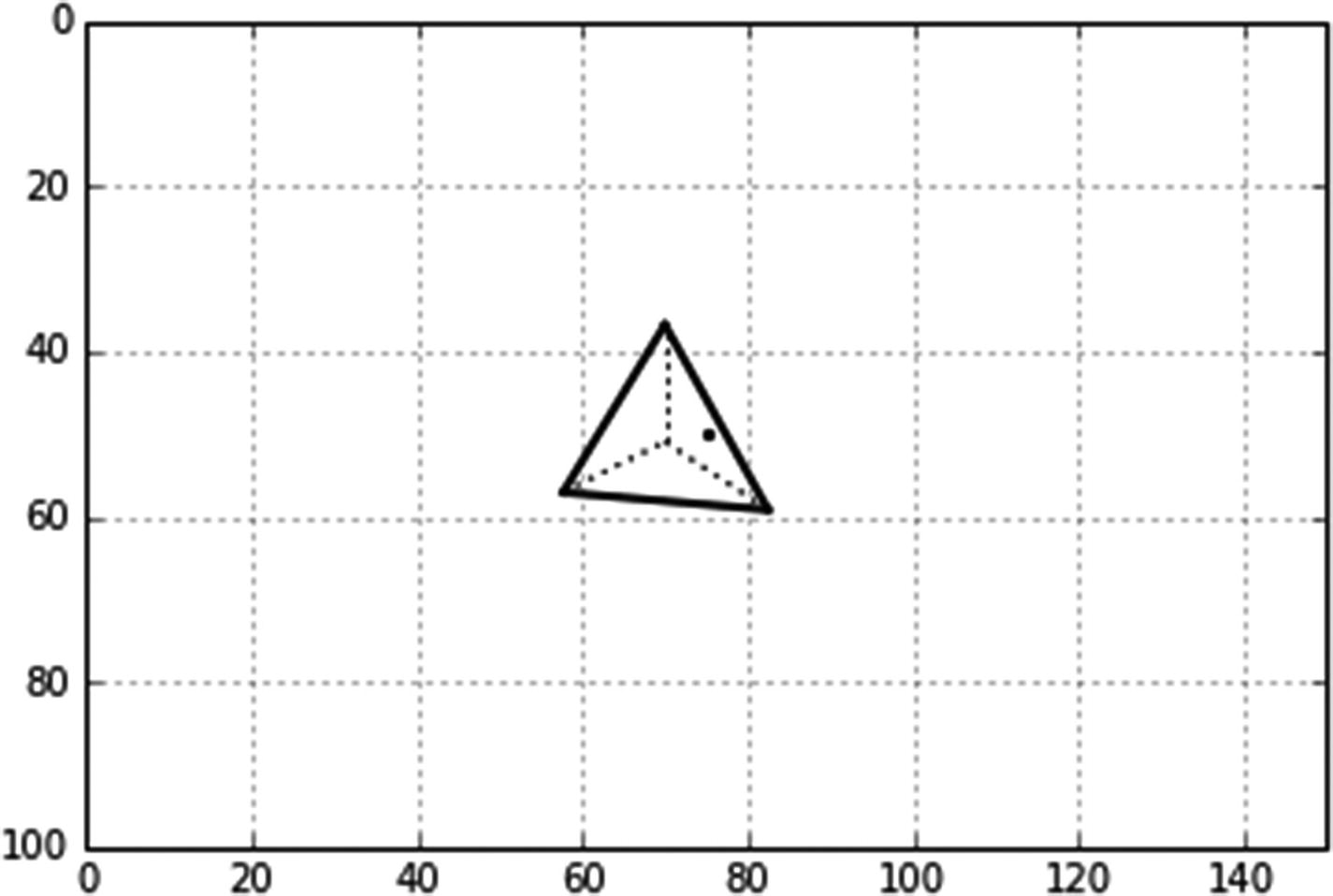
Model for Listing 6-2. N not to scale.

1   """
2   HLPYRAMID
3   """
4
5   import numpy as np
6   import matplotlib.pyplot as plt
7   from math import sin, cos, radians
8   #————————————————————define lists
9   x=[0,-10,0,10]
10  y=[-20,0,0,0]
11  z=[0,10,-15,10]
12
13  xg=[0]*len(x)
14  yg=[0]*len(x)
15  zg=[0]*len(x)
16
17  #============================================define rotation function
18  def rotx(xc,yc,zc,xp,yp,zp,Rx):
19       xpp=xp
20       ypp=yp*cos(Rx)-zp*sin(Rx)
21       zpp=yp*sin(Rx)+zp*cos(Rx)
22       [xg,yg,zg]=[xpp+xc,ypp+yc,zpp+zc]
23       return[xg,yg,zg]
24
25  def roty(xc,yc,zc,xp,yp,zp,Ry):
26       xpp=xp*cos(Ry)+zp*sin(Ry)
27       ypp=yp
28       zpp=-xp*sin(Ry)+zp*cos(Ry)
29       [xg,yg,zg]=[xpp+xc,ypp+yc,zpp+zc]
30       return[xg,yg,zg]
31
32  def rotz(xc,yc,zc,xp,yp,zp,Rz):
33       xpp=xp*cos(Rz)-yp*sin(Rz)
34       ypp=xp*sin(Rz)+yp*cos(Rz)
35       zpp=zp
36       [xg,yg,zg]=[xpp+xc,ypp+yc,zpp+zc]
37       return[xg,yg,zg]
38
39  #======================================define pyramid plotting function
40
41  def plotpyramid(xg,yg,zg):
42       v01x=x[1]-x[0] #———0,1,2 face
43       v01y=y[1]-y[0]
44       v01z=z[1]-z[0]
45       v02x=x[2]-x[0]
46       v02y=y[2]-y[0]
47       v02z=z[2]-z[0]
48       nz=v01x*v02y-v01y*v02x
49       if nz<=0 :
50            plt.plot([xg[0],xg[1]],[yg[0],yg[1]],color='k',linewidth=2)
51            plt.plot([xg[1],xg[2]],[yg[1],yg[2]],color='k',linewidth=2)
52            plt.plot([xg[2],xg[0]],[yg[2],yg[0]],color='k',linewidth=2)
53       else:
54            plt.plot([xg[0],xg[1]],[yg[0],yg[1]],color='k',linestyle=':')
55            plt.plot([xg[1],xg[2]],[yg[1],yg[2]],color='k',linestyle=':')
56            plt.plot([xg[2],xg[0]],[yg[2],yg[0]],color='k',linestyle=':')
57
58       v03x=x[3]-x[0] #—0,2,3 face
59       v03y=y[3]-y[0]
60       v03z=z[3]-z[0]
61       nz=v02x*v03y-v02y*v03x
62       if nz<=0 :
63            plt.plot([xg[0],xg[2]],[yg[0],yg[2]],color='k',linewidth=2)
64            plt.plot([xg[0],xg[3]],[yg[0],yg[3]],color='k',linewidth=2)
65            plt.plot([xg[2],xg[3]],[yg[2],yg[3]],color='k',linewidth=2)
66       else:
67            plt.plot([xg[0],xg[2]],[yg[0],yg[2]],color='k',linestyle=':')
68            plt.plot([xg[0],xg[3]],[yg[0],yg[3]],color='k',linestyle=':')
69            plt.plot([xg[2],xg[3]],[yg[2],yg[3]],color='k',linestyle=':')
70
71       nz=v03x*v01y-v03y*v01x #—0,2,3 face
72       if nz<=0 :
73            plt.plot([xg[0],xg[1]],[yg[0],yg[1]],color='k',linewidth=2)
74            plt.plot([xg[0],xg[3]],[yg[0],yg[3]],color='k',linewidth=2)
75            plt.plot([xg[1],xg[3]],[yg[1],yg[3]],color='k',linewidth=2)
76       else:
77            plt.plot([xg[0],xg[1]],[yg[0],yg[1]],color='k',linestyle=':')
78            plt.plot([xg[0],xg[3]],[yg[0],yg[3]],color='k',linestyle=':')
79            plt.plot([xg[1],xg[3]],[yg[1],yg[3]],color='k',linestyle=':')
80
81       v21x=x[1]-x[2] #———1,2,3 face
82       v21y=y[1]-y[2]
83       v21z=z[1]-z[2]
84       v23x=x[3]-x[2]
85       v23y=y[3]-y[2]
86       v23z=z[3]-z[2]
87       nz=v21x*v23y-v21y*v23x
88       if nz¡0:
89            plt.plot([x[2],x[1]],[y[2],y[1]])
90            plt.plot([x[1],x[3]],[y[1],y[3]])
91            plt.plot([x[3],x[2]],[y[3],y[2]])
92
93       plt.scatter(xc,yc,s=5,color='k') #———plot a dot at the center
94       plt.axis([0,150,100,0]) #———replot axes and grid
95       plt.axis('on')
96       plt.grid(True)
97       plt.show() #–plot latest rotation
98
99  #========================transform coordinates and plotting fucntions
100 def plotpyramidx(xc,yc,zc,Rx): #——————transform & plot Rx pyramid
101      for i in range(len(x)):
102            [xg[i],yg[i],zg[i]]=rotx(xc,yc,zc,x[i],y[i],z[i],Rx) 
103            [x[i],y[i],z[i]]=[xg[i]-xc,yg[i]-yc,zg[i]-zc]
104
105      plotpyramid(xg,yg,zg) #—————plot
106
107 def plotpyramidy(xc,yc,zc,Ry):
108      for i in range(len(x)): #——————transform & plot Ry pyramid
109            [xg[i],yg[i],zg[i]]=roty(xc,yc,zc,x[i],y[i],z[i],Ry)
110            [x[i],y[i],z[i]]=[xg[i]-xc,yg[i]-yc,zg[i]-zc]
111
112      plotpyramid(xg,yg,zg)
113
114 def plotpyramidz(xc,yc,zc,Rz):
115      for i in range(len(x)): #——————transform & plot Rz pyramid
116            [xg[i],yg[i],zg[i]]=rotz(xc,yc,zc,x[i],y[i],z[i],Rz)
117            [x[i],y[i],z[i]]=[xg[i]-xc,yg[i]-yc,zg[i]-zc]
118
119      plotpyramid(xg,yg,zg)
120
121 #———————————————————plot pyramids
122 xc=75 #——center coordinates
123 yc=50
124 zc=50
125
126 while True:
127      axis=input('x, y or z?: ') #———input axis of rotation (lower case)
128      if axis == 'x': #———if x axis
129            Rx=radians(float(input('Rx Degrees?: '))) #———input degrees of rotation
130            plotpyramidx(xc,yc,zc,Rx) #———call function plotpyramidx
131      if axis == 'y':
132            Ry=radians(float(input('Ry Degrees?: '))) #———input degrees of rotation
133            plotpyramidy(xc,yc,zc,Ry)
134      if axis == 'z':
135            Rz=radians(float(input('Rz Degrees?: '))) #———input degrees of rotation
136            plotpyramidz(xc,yc,zc,Rz)
137      if axis == ":
138            break
Listing 6-2

Program HLPYRAMID

6.3 Planes

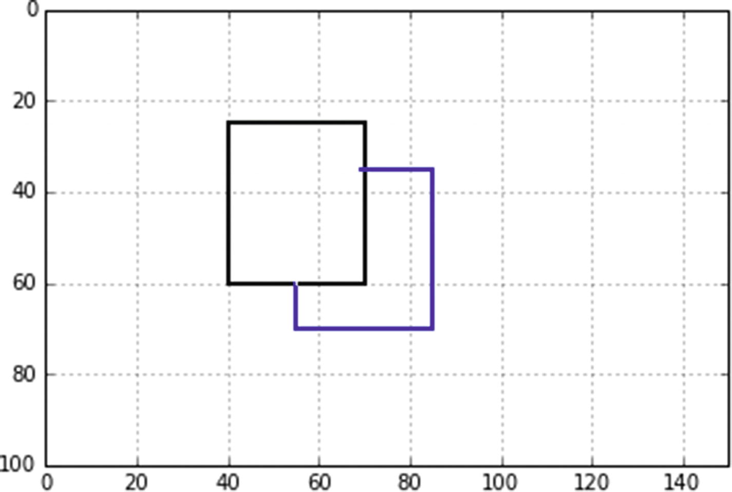
Next is an example of inter-object hidden line removal. Figure 6-9 shows two planes, (a) and (b); Figure 6-10 shows the same two planes partially overlapping. As you will see shortly, plane (b) is actually beneath the plane (a) and should be partially obscured. Figures 6-11 shows the planes with the hidden lines of plane (b) removed. Figure 6-12 shows another example. Figure 6-13 shows an example with plane (a) rotated.

In this simple model, the two planes are parallel to the x,y plane with plane (b) taken to be located behind plane (a) (i.e. further in the +z direction). You do not need to be concerned with the z component of the planes’ coordinates since you won’t be rotating them out of plane, (i.e. around the x or y directions), although you will be rotating plane (a) in its plane around the z direction, but for this you do not need z coordinates.

Figure 6-14 shows the model used by Listing 6-3. Plane (a) is drawn in black, plane (b) in blue. Unit vectors î and jˆ are shown at corner 0 of plane (a). You use a ray tracing technique to remove the hidden lines when plane (b) or part of it is behind (a) and not visible. You do so line by line beginning with edge 0-1 of plane (b). Starting at corner 0 of plane (b), you imagine a ray emitting from that point travelling to an observer who is located in the -z direction and looking in onto the x,y plane. If plane (a) does not interfere with that ray (i.e. does not cover up that point), the dot is plotted. If plane (a) does interfere, it is not plotted. The problem thus become one of intersections: determining if a ray from a point on an edge of plane (b) intersects plane (a).

The edges of plane (b) are processed one at a time. Starting with corner 0, you proceed along edge 0-1 to corner 1 in small steps. Vector H shows the location of a point h on edge 0-1. Listing 6-3 determines the location of this point and whether or not it lies beneath plane (a) (i.e. if a ray emanating from h strikes plane (a)). If it does not, point p is plotted; if it does, p is not plotted.

In Listing 6-3, lines 14-18 establish the coordinates of the two planes in global coordinates, ready for plotting. Lines 21-32 define a function, dlinea, that plots the edge lines of plane (a). It does so one edge line at a time. dlinea does not do a hidden line check on the edges of plane (a) since you are stipulating that plane (a) lies over plane (b). The calling arguments x1,x2,y1,y2 are the beginning and end coordinates of the edge line. q in line 22 is the length of that line; uxa and uya are the x and y components of a unit vector that points along the edge line from x1,y1 to x2,y2. The loop in lines 27-32 advances the point along the line from x1,y1 to x2,y2 in steps of .2 as set in line 27. hx and hy in lines 28 and 29 are the coordinates of point h along the line. hxstart and hystart permit connecting the points by short line segments, giving a finer appearance than if the points were plotted as dots.

Lines 35-38 plot the edges of plane (a) by calling function dlinea with the beginning and end coordinates of each of the four edges. Lines 40-42 establish the distance qa03 from corner 0 of plane (a) to corner 3. uxa and uya in lines 43 and 44 are the x and y components of a unit vector û, which points from corner 0 to corner 3. Similarly, lines 46-50 give the components of $$ widehat{mathbf{v}} $$, a unit vector pointing from corner 0 to 1. They will be required to do the intersection check, as was done in the preceding chapter with line/plane intersections.

Function dlineb is similar to dlinea except the calling arguments now include agx[0] and agy[0], the coordinates of corner 0 of plane (a). Also, this function includes the interference check, which is between lines 64 and 71. This is labelled the inside/outside check. In line 64, a is the distance between the x coordinate of point h and the x coordinate of corner 0 of plane (a); b in line 65 is the y distance. These are essentially the x and y components of vector H. In line 66, the dot (scalar) product of H with unit vector û gives up. This is the projection of H on the 0-3 side of plane (a). Similarly, the dot product of H with unit vector $$ widehat{mathbf{v}} $$ in line 67 gives vp, the projection of H on the 0-1 side of plane (a). The interference check is then straightforward and is summarized in line 68. If all questions in line 68 are true, the point is plotted in line 69 in white, which means it is invisible. If any the questions in line 68 are false, which means the point is not blocked by plane (a), line 71 plots it in black.

You may ask, why use this elaborate vector analysis? Why not just check each point’s x and y coordinates as shown in Figure 6-14 against the horizontal and vertical boundaries of plane (a)? You could do that if both planes remain aligned with the x and y axes as shown. But by using the vector approach, you enable either one of the planes to be rotated about the z direction as shown in Figure 6-13.

I have simplified this model a bit by specifying that plane (b) lie under (a). In general, you may not know which plane is closer to the observer and which should be (a) and which (b). This can be accomplished by a simple check on z coordinates. In principle, the hidden line removal process would be similar to what you have done here, although the programming can get complicated trying to keep track of a large assemblage of objects.
../images/456962_1_En_6_Chapter/456962_1_En_6_Fig9_HTML.jpg
Figure 6-9

Two planes

../images/456962_1_En_6_Chapter/456962_1_En_6_Fig10_HTML.jpg
Figure 6-10

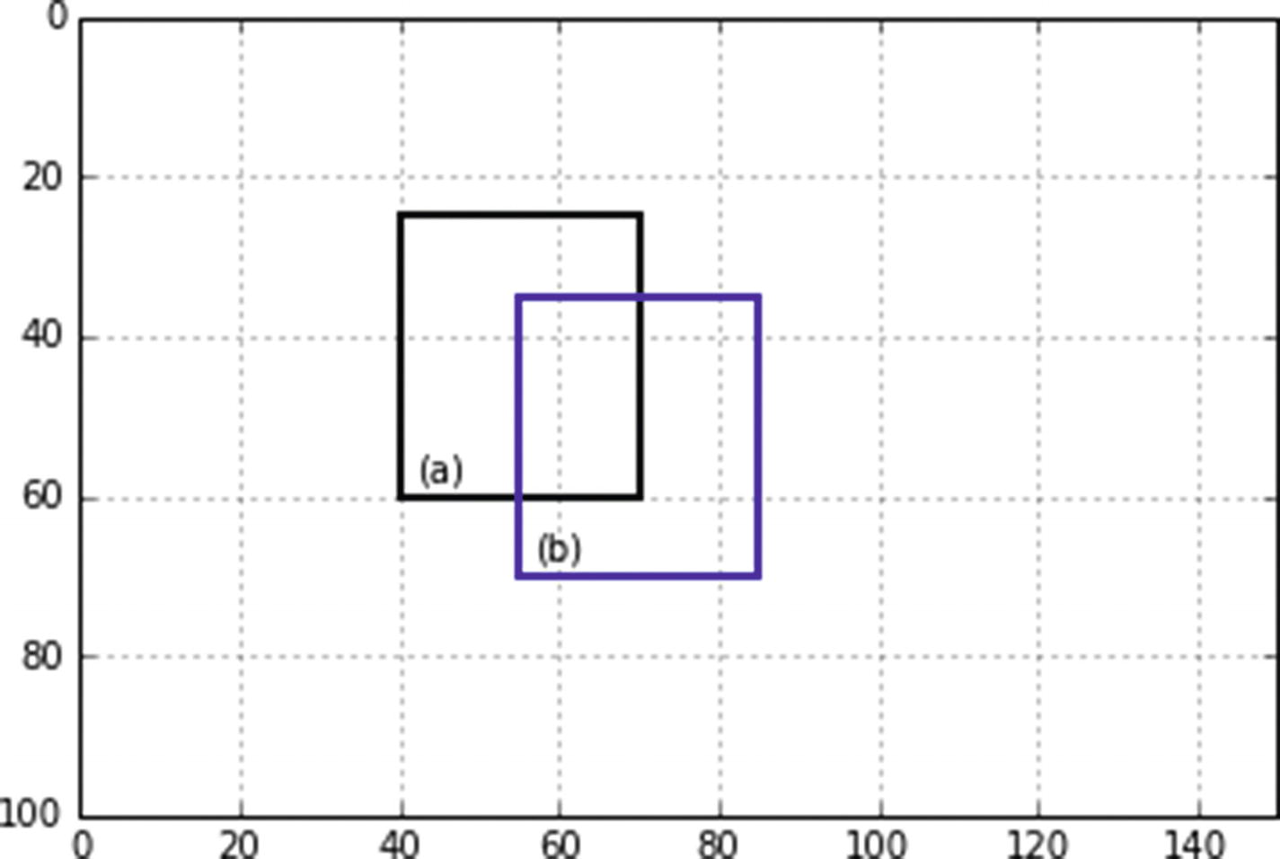
Two planes, one partially overlapping the other, hidden lines not removed. Plane (b) is beneath (a).

../images/456962_1_En_6_Chapter/456962_1_En_6_Fig11_HTML.jpg
Figure 6-11

Two planes overlapping, hidden lines removed by Listing 6-3

../images/456962_1_En_6_Chapter/456962_1_En_6_Fig12_HTML.jpg
Figure 6-12

Two planes, one overlapping the other, hidden lines removed by Listing 6-3

../images/456962_1_En_6_Chapter/456962_1_En_6_Fig13_HTML.jpg
Figure 6-13

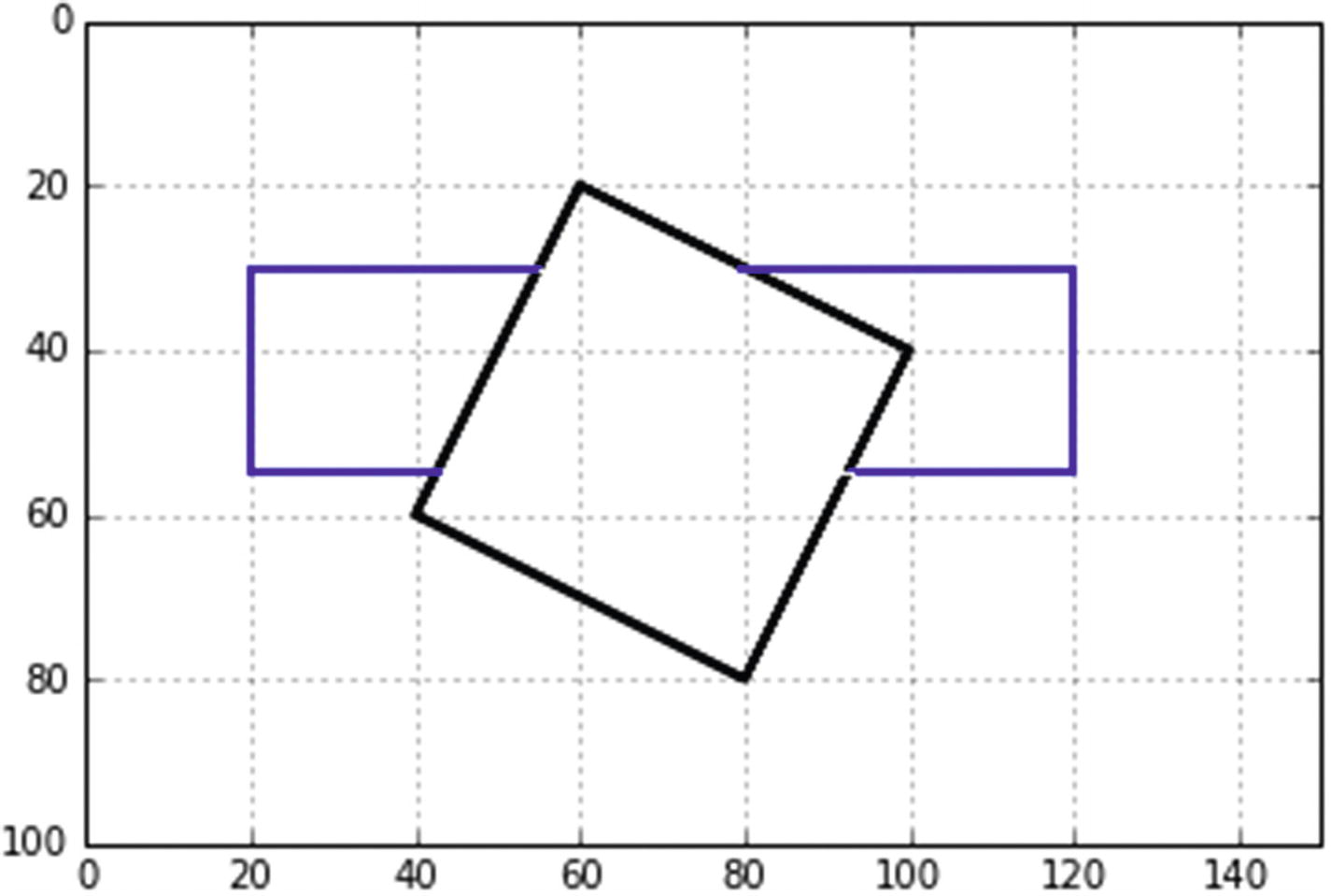
Two planes, one at an angle and overlapping the other, hidden lines removed by Listing 6-3

../images/456962_1_En_6_Chapter/456962_1_En_6_Fig14_HTML.jpg
Figure 6-14

Model for Listing 6-3

1   """
2   HLPLANES
3   """
4
5   import numpy as np
6   import matplotlib.pyplot as plt
7   from math import sqrt, sin, cos, radians
8
9   plt.axis([0,150,100,0])
10  plt.axis('off')
11  plt.grid(False)
12
13  #———————————————————-define lists
14  axg=[40,80,80,40]
15  ayg=[20,20,60,60]
16
17  bxg=[20,120,120,20]
18  byg=[30,30,55,55]
19
20  #================================================define function dlinea
21  def dlinea(x1,x2,y1,y2):
22       q=sqrt((x2-x1)**2+(y2-y1)**2)
23       uxa=(x2-x1)/q
24       uya=(y2-y1)/q
25       hxstart=x1
26       hystart=y1
27       for l in np.arange(0,q,.2):
28              hx=x1+l*uxa #———global hit coordinates along the line
29              hy=y1+l*uya
30              plt.plot([hxstart,hx],[hystart,hy],color='k')
31              hxstart=hx
32              hystart=hy
33
34  #—————————————————————plane (a)
35  dlinea(axg[0],axg[1],ayg[0],ayg[1]) #———plot plane (a)
36  dlinea(axg[1],axg[2],ayg[1],ayg[2])
37  dlinea(axg[2],axg[3],ayg[2],ayg[3])
38  dlinea(axg[3],axg[0],ayg[3],ayg[0])
39
40  a=axg[3]-axg[0] #———unit vector u plane (a)
41  b=ayg[3]-ayg[0]
42  qa03=sqrt(a*a+b*b)
43  uxa=a/qa03
44  uya=b/qa03
45
46  a=axg[1]-axg[0] #———unit vector v plane (a)
47  b=ayg[1]-ayg[0]
48  qa01=sqrt(a*a+b*b)
49  vxa=a/qa01
50  vya=b/qa01
51
52  #=============================================================lineb( )
53  def dlineb(x1,x2,y1,y2,ax0,ay0):
54       a=x2-x1 #———unit vector line
55       b=y2-y1
56       ql=sqrt(a*a+b*b)
57       uxl=a/ql
58       uyl=b/ql
59       hxglast=x1
60       hyglast=y1
61       for l in np.arange(0,ql,.5):
62             hxg=x1+l*uxl
63             hyg=y1+l*uyl
64             a=hxg-ax0 #———inside/outside check
65             b=hyg-ay0
66             up=a*uxa+b*uya
67             vp=a*vxa+b*vya
68             if 0<up<qa03 and 0<vp<qa01: #———is it inside (a)?
79                  plt.plot([hxglast,hxg],[hyglast,hyg],color=’white’)
70             else:
71                  plt.plot([hxglast,hxg],[hyglast,hyg],color=’k’)
72       hxglast=hxg
73       hyglast=hyg
74
75  #———————————————————plot plane (b)
76  dlineb(bxg[0],bxg[1],byg[0],byg[1],axg[0],ayg[0])
77  dlineb(bxg[1],bxg[2],byg[1],byg[2],axg[0],ayg[0])
78  dlineb(bxg[2],bxg[3],byg[2],byg[3],axg[0],ayg[0])
79  dlineb(bxg[3],bxg[0],byg[3],byg[0],axg[0],ayg[0])
80
81  plt.show()
Listing 6-3

Program HLPLANES

6.4 Sphere

In Chapter 5, you drew a sphere but did not rotate it. The lines on the back side were overlapped by those on the front and thus weren’t visible, so removing hidden lines was not an issue. In this chapter, you will draw a sphere and rotate it while removing hidden lines on the back side.

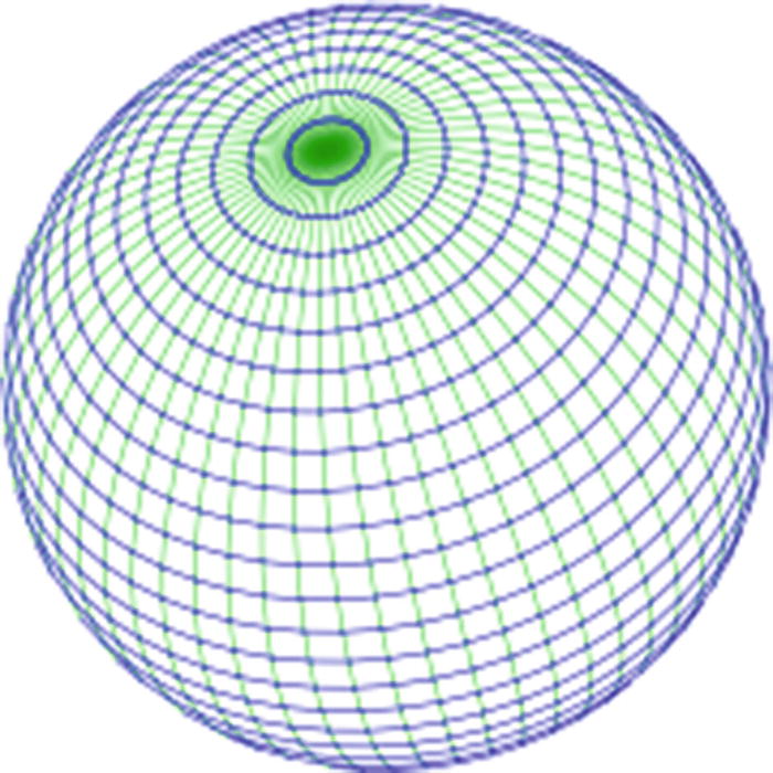
Figures 6-15 and 6-18 show examples of the output from Listing 6-4, which plots a sphere with hidden lines removed. The vertical lines in Figures 6-15 and 6-16, the longitudes, are drawn in green; the horizontal latitudes are drawn in blue. The program uses a hidden line removal scheme much like the one you used before with boxes and pyramids. If the z component of a vector perpendicular to a point is positive (i.e. pointing away from an observer who is located in the -z direction), the point is not drawn; otherwise it is drawn.

In Listing 6-4, line 14 sets the length of the list g[] to 3. This will be used to return global coordinates xg,yg, and zg from the rotation functions rotx, roty, and rotz, which are defined in lines 24-40 (they are the same as the functions used in previous programs). The longitudes are plotted in lines 55-79. The model is the same as used in Listing 5-5 in Chapter 5. The algorithm between lines 55 and 79 calculates the location of each point on a longitude, one at a time, and rotates it. That is, each point is established and rotated separately; lists are not used other than the g[ ] list. The alpha loop starting in line 55 sweeps the longitudes from α = 0 to α = 360 in six-degree steps as set in lines 47-49. At each α step a longitude is drawn by the ϕ loop, which starts at -90 degrees and goes to +90 in six-degree steps. The geometry in lines 57-59 is taken from Listing 5-5. The coordinates of a point before rotation (Rx=0, Ry=0, Rz=0) are xp,yp,zp as shown in lines 57-59. This point is located on the sphere’s surface at spherical coordinates α, ϕ. Line 60 rotates the point about the x direction by an angle Rx. This produces new coordinates xp,yp,zp in lines 61-63. Line 64 rotates the point at these new coordinates around the y direction. Line 68 rotates it around the z direction. This produces the final location of the point.

Next, you must determine whether or not the point is on the back side of the sphere and hidden from view. If true, it is not plotted. Lines 73-79 perform this function. First, in lines 73-75, you establish the starting coordinates of the line that will connect the first point to the second. You use lines to connect the points rather than dots since lines give a finer appearance. Line 73 asks if phi equals phi1, the starting angle in the phi loop. If it does, the starting coordinates xpglast and ypglast are set equal to the first coordinates calculated by the loop. Next, in line 76, you ask if nz, the z component of a vector from the sphere’s center to the point, is less than 0. nz is calculated in line 72. If true, you know the point is visible to an observer situated in the -z direction; the point is then connected to the previous one by line 77.

The plt.plot() function in line 77 needs two sets of coordinates: xpglast,ypglast and xpg,ypg. During the first cycle through the loop, the starting coordinates xpglast,ypglast are set equal to xpg,ypg, meaning the first point is connected to itself so the first line plotted will have zero length. After that, the coordinates of the previous point are set in lines 78-79. Line 73 determines if it is the first point. If nz is greater than zero in line 76, the point is on the back side of the rotated sphere and is not visible so it is not plotted. The coordinates xpglast and ypglast must still be updated and this is done in lines 78-79. The latitudes are processed in much the same way, although the geometry is different, as described in Listing 5-5. The colors of the longitudes and latitudes can be changed by changing the color='color' values in lines 77 and 104.

When running this program, remember that the rotations are not additive as in some of the previous programs. The angles of rotation specified in lines 51-53 are the angles the sphere will end up at; they are not added to any previous rotations. To rotate the sphere to another orientation, change the values in lines 51-53.

As mentioned in the discussion on concatenation, the sequence of rotations is important. Rx followed by Ry does not give the same results as Ry followed by Rx. This program has the sequence of function calls, Rx,Ry,Rz, as specified in lines 60, 64, and 68 for longitudes and 87, 91, and 95 for latitudes. To change the order of rotation, change the order of these function calls.

The spheres shown in Figures 6-17 and 6-18 have a black background. To achieve this, insert the following lines in Listing 6-4 before any other plotting commands, for example after line 12:

#———————————————————paint the background
for y in np.arange(1,100,1):
     plt.plot([0,150],[y,y],linewidth=4,color='k')

This plots black lines across the plotting window from x=0 to x=150 and down from y=1 to y=100. This fills the area with a black background. The color can be changed to anything desired. The linewidth has been set to 4 in order to prevent gaps from appearing between the horizontal lines. The background must be painted before constructing the sphere since you are using line segments to do that. New lines overplot old ones, so with this order the sphere line segments will overplot the background lines; otherwise the background lines would overplot the sphere.

In Figures 6-15 and 6-16, the sphere’s line widths in program lines 77 and 104 is set to .5. This gives good results on a clear background but the lines are too subdued when the background is changed to black. So, along with inserting the two lines of code above, the line widths in Listing 6-4 should be changed to something greater such as 1.0. The color shown in Figures 6-17 and 6-18 is 'lightgreen'. Some colors don’t plot well against a black background but color='lightgreen' seems to work; you just have to experiment.

1   """
2   HLSPHERE
3   """
4
5   import numpy as np
6   import matplotlib.pyplot as plt
7   from math import sin, cos, radians, sqrt
8
9   plt.axis([0,150,100,0])
10  plt.axis('off')
11  plt.grid(False)
12
13  #———————————————————————lists
14  g=[0]*3
15
16  #—————————————————————parameters
17  xc=80 #———sphere center
18  yc=50
19  zc=0
20
21  rs=40 #———sphere radius
22
23  #=========================================================
24  def rotx(xc,yc,zc,xp,yp,zp,Rx):
25       g[0]=xp+xc
26       g[1]=yp*cos(Rx)-zp*sin(Rx)+yc
27       g[2]=yp*sin(Rx)+zp*cos(Rx)+zc
28       return[g]
29
30  def roty(xc,yc,zc,xp,yp,zp,Ry):
31       g[0]=xp*cos(Ry)+zp*sin(Ry)+xc
32       g[1]=yp+yc
33       g[2]=-xp*sin(Ry)+zp*cos(Ry)+zc
34       return[g]
35
36  def rotz(xc,yc,zc,xp,yp,zp,Rz):
37       g[0]=xp*cos(Rz)-yp*sin(Rz)+xc
38       g[1]=xp*sin(Rz)+yp*cos(Rz)+yc
39       g[2]=zp+zc
40       return[g]
41
42  #————————————————-longitudes and latitudes
43  phi1=radians(-90)
44  phi2=radians(90)
45  dphi=radians(6)
46
47  alpha1=radians(0)
48  alpha2=radians(360)
49  dalpha=radians(6)
50
51  Rx=radians(45)
52  Ry=radians(-20)
53  Rz=radians(40)
54
55  for alpha in np.arange(alpha1,alpha2,dalpha):  #———longitudes
56       for phi in np.arange(phi1,phi2,dphi):
57            xp=rs*cos(phi)*cos(alpha)
58            yp=rs*sin(phi)
59            zp=-rs*cos(phi)*sin(alpha)
60            rotx(xc,yc,zc,xp,yp,zp,Rx)
61            xp=g[0]-xc
62            yp=g[1]-yc
63            zp=g[2]-zc
64            roty(xc,yc,zc,xp,yp,zp,Ry)
65            xp=g[0]-xc
66            yp=g[1]-yc
67            zp=g[2]-zc
68            rotz(xc,yc,zc,xp,yp,zp,Rz)
69            xpg=g[0]
70            ypg=g[1]
71            zpg=g[2]
72            nz=zpg-zc
73            if phi == phi1:
74                   xpglast=xpg
75                   ypglast=ypg
76            if nz < 0:
77                   plt.plot([xpglast,xpg],[ypglast,ypg],linewidth=.5,color='g')
78            xpglast=xpg
79            ypglast=ypg
80
81  for phi in np.arange(phi1,phi2,dphi):  #—————latitudes
82       r=rs*cos(phi)
83       for alpha in np.arange(alpha1,alpha2+dalpha,dalpha):
84            xp=r*cos(alpha)
85            yp=rs*sin(phi)
86            zp=-rs*cos(phi)*sin(alpha)
87            rotx(xc,yc,zc,xp,yp,zp,Rx)
88            xp=g[0]-xc
89            yp=g[1]-yc
90            zp=g[2]-zc
91            roty(xc,yc,zc,xp,yp,zp,Ry)
92            xp=g[0]-xc
93            yp=g[1]-yc
94            zp=g[2]-zc
95            rotz(xc,yc,zc,xp,yp,zp,Rz)
96            xpg=g[0]
97            ypg=g[1]
98            zpg=g[2]
99            nz=zpg-zc
100           if alpha == alpha1:
101                  xpglast=xpg
102                  ypglast=ypg
103           if nz < 0:
104                   plt.plot([xpglast,xpg],[ypglast,ypg],linewidth=.5,color='b')
105           xpglast=xpg
106           ypglast=ypg
107
108 plt.show()
Listing 6-4

Program HLSPHERE

../images/456962_1_En_6_Chapter/456962_1_En_6_Fig15_HTML.jpg
Figure 6-15

Rotated sphere with hidden lines removed: Rx=55°, Ry=-20°, Rz=-40° (produced by Listing 6-4)

../images/456962_1_En_6_Chapter/456962_1_En_6_Fig16_HTML.jpg
Figure 6-16

Rotated sphere with hidden lines removed: Rx=40°, Ry=-20°, Rz=40° (produced by Listing 6-4)

../images/456962_1_En_6_Chapter/456962_1_En_6_Fig17_HTML.jpg
Figure 6-17

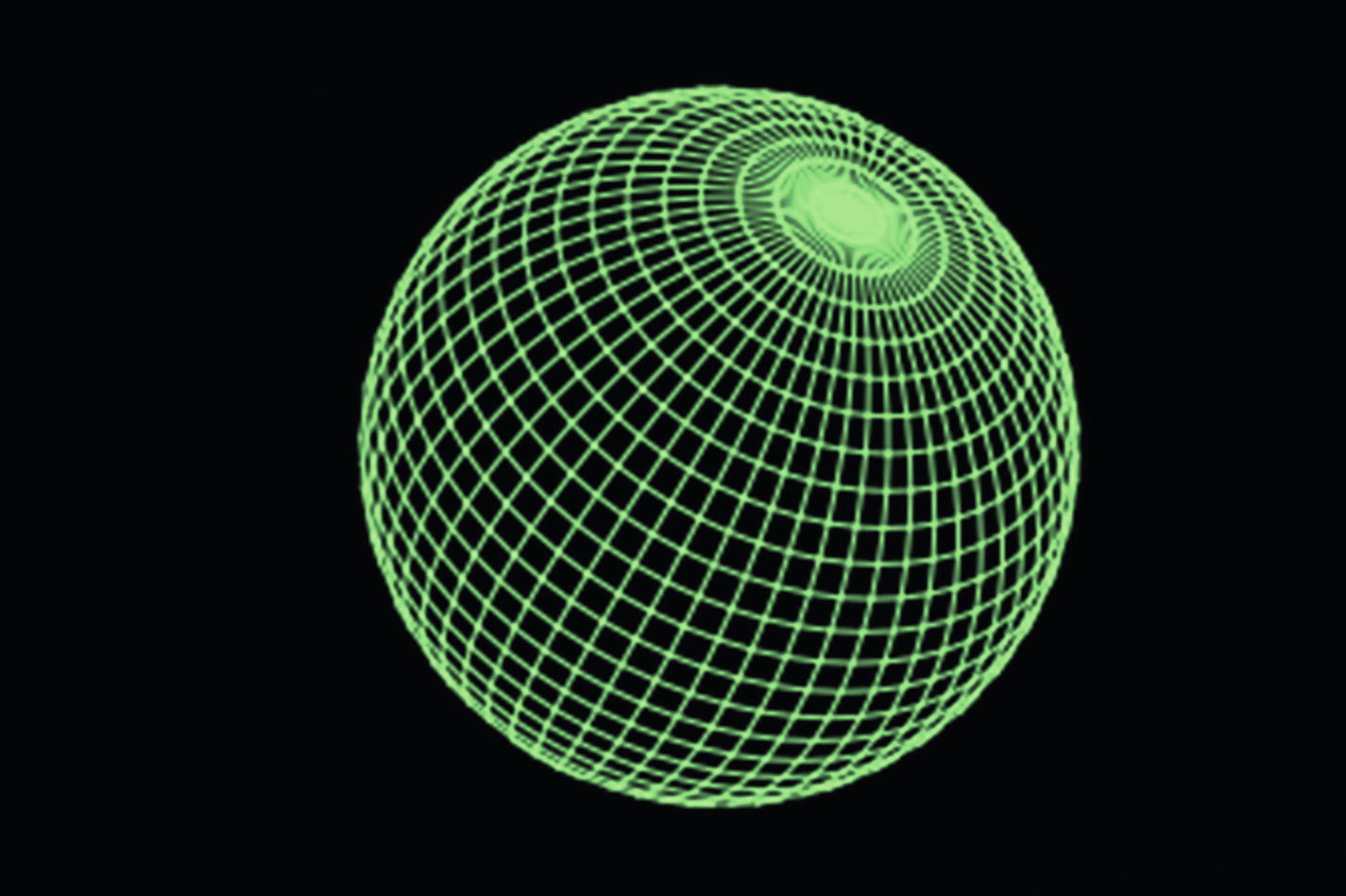
Rotated sphere with hidden lines removed: Rx=40°, Ry=-20°, Rz=40°, black background (produced by Listing 6-4)

../images/456962_1_En_6_Chapter/456962_1_En_6_Fig18_HTML.jpg
Figure 6-18

Rotated sphere with hidden lines removed: Rx=60°, Ry=20°, Rz=10°, black background (produced by Listing 6-4)

6.5 Summary

You learned how to remove hidden lines from single objects and between objects. In the case of single objects, such as the box, the pyramid, and the sphere, you were able to construct algorithms without much trouble. When removing hidden lines from separate objects, such as two planes, you relied on the technique of constructing one of the objects from dots or short line segments that go from one dot to another. In either case, you were still dealing with dots. From a dot on one plane, you drew an imaginary line, a ray, to an observer in the -z direction. Then you checked to see if the ray intersected the other plane. You used the line-plane intersection algorithm developed in Chapter 5. If it did intersect, the dot was hidden and it, or a line segment connected to it, was not drawn. You used two planes to explore this technique. You could have used any of the other shapes you worked with in Chapter 5. For example, you could have easily removed hidden lines from a plane beneath a circular segment by constructing the plane from dots and using the intersection algorithm from Chapter 5. However, you might not know ahead of time which object covers which. You could do a rough check to answer this question. For example, in the case of two planes, if the z coordinates of all four corners of one plane are less than the other, it is closer to the observer, in which case it may cover part of the other plane. In this case, the other plane should be checked for hidden lines.

..................Content has been hidden....................

You can't read the all page of ebook, please click here login for view all page.
Reset
3.140.198.43