© B.J. Korites 2018
B.J. KoritesPython Graphicshttps://doi.org/10.1007/978-1-4842-3378-8_2

2. Graphics in Two Dimensions

B. J. Korites1 
(1)
Duxbury, Massachusetts, USA
 

In this chapter, you will learn how to construct two-dimensional images using points and lines. You learned the basic tools for creating images with Python in Chapter 1. In this chapter, you will expand on that and learn methods to create, translate and rotate shapes in two dimensions. You will also learn about the concept of relative coordinates, which will be used extensively throughout the remainder of this book. As usual, you will explore these concepts through sample programs.

2.1 Lines from Dots

You saw how to create a line with the command

plt.plot([x1,x2],[y1,y2],attributes)

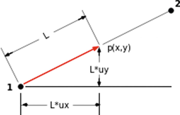
This draws a line from (x1,y1) to (x2,y2) with attributes specifying the line’s width, color, and style. At times it may be desirable to construct a line using dots. Figures 2-1 and 2-2 show the geometry: an inclined line beginning at point 1 and ending at point 2. Its length is Q. Shown on the line in Figure 2-2 is point p at coordinates x,y. To draw the line, you start at 1 and advance toward 2 in steps, calculating coordinates of p at each step and plotting a dot at each step as you go. This analysis utilizes vectors, which will be used extensively later.

Note that you do not have coordinate axes in these models. This analysis is generic; it is applicable to any two-dimensional orthogonal coordinate directions.

../images/456962_1_En_2_Chapter/456962_1_En_2_Fig1_HTML.jpg
Figure 2-1

Geometry for creating a line from dots (a)

../images/456962_1_En_2_Chapter/456962_1_En_2_Fig2_HTML.jpg
Figure 2-2

Geometry for creating a line from dots (b)

To advance from point 1 toward point 2, you must first determine the direction from 1 to 2. This will be expressed as a unit vector û (unit vectors will be shown in bold with a hat; full vectors in bold):
$$ widehat{mathbf{u}}=uxwidehat{mathbf{i}}+uywidehat{mathbf{j}} $$
(2-1)
where and are unit vectors in the x and y directions; ux and uy are the scalar components of û in the x and y directions.

ux is the cosine of the angle between û and the x axis; uy is the cosine of the angle between û and the y axis. ux and uy are often referred to as direction cosines. It is easy to show they are cosines: the cosine of the angle between û and the x axis is ux/|û| , where |û| is the scalar magnitude of û. Since û is a unit vector, |û|=1;. The cosine of the angle is then ux/(1)=ux. Similarly for uy.

It is important to remember that
$$ left|widehat{mathbf{u}}
ight|=1 $$
(2-2)
since this feature enables you to multiply û by a magnitude to get a position vector. For example, you can get a vector from point 1 to p, v1p, by multiplying û by L where L is the distance from 1 to p. L gives the vector its magnitude, û gives its direction. A vector from point 1 to p is then
$$ mathbf{v}mathbf{l}mathbf{p}=Lleft(ux;widehat{mathbf{i}}+uy;widehat{mathbf{j}}
ight) $$
(2-3)
You can calculate ux and uy from coordinate values as
$$ ux=A/Q=left(x2hbox{-} x1
ight)/Q $$
(2-4)
$$ uy=B/Q=left(y2hbox{-} y1
ight)/Q $$
(2-5)
where (x1,y1) and (x2,y2) are the coordinates of points 1 and 2, and
$$ Q=sqrt{{left(x2hbox{-} x1
ight)}^2+{left(y2hbox{-} y1
ight)}^2} $$
(2-6)
Listing 2-1 gives two examples of lines drawn with dots. The results are shown in Figure 2-3. Smaller dots and closer spacing will produce a finer line (green), which is almost as good the line obtained by using the plt.plot([x1,x2],[y1,y2]) function.
../images/456962_1_En_2_Chapter/456962_1_En_2_Fig3_HTML.jpg
Figure 2-3

Dot lines created by Listing 2-1

1   """
2   DOTLINE
3   """
4
5   import matplotlib.pyplot as plt
6   import numpy as np
7
8   plt.axis([-20,130,80,-20])
9
10  plt.axis('on')
11  plt.grid(True)
12
13  plt.arrow(0,0,20,0,head_length=4,head_width=3,color='k')
14  plt.arrow(0,0,0,20,head_length=4,head_width=3,color='k')
15  plt.text(15,-3,'x')
16  plt.text(-5,15,'y')
17
18  #———————————————————green line
19  x1=20
20  x2=120
21  y1=40
22  y2=20
23
24  q=np.sqrt((x2-x1)**2+(y2-y1)**2)
25  ux=(x2-x1)/q
26  uy=(y2-y1)/q
27
28  for l in np.arange(0,q,.5):
29        px=x1+l*ux
30        py=y1+l*uy
31        plt.scatter(px,py,s=1,color='g')
32
33  #———————————————————————————————————————————blue line
34  x1=20
35  x2=120
36  y1=45
37  y2=25
38
39  q=np.sqrt((x2-x1)**2+(y2-y1)**2)
40  ux=(x2-x1)/q
41  uy=(y2-y1)/q
42
43  for l in np.arange(0,q,2):
44        px=x1+l*ux
45        py=y1+l*uy
46        plt.scatter(px,py,s=1,color='b')
47
48  plt.show()
Listing 2-1

Program DOTLINE

This program should be self-explanatory since the definitions are consistent with the prior analysis.
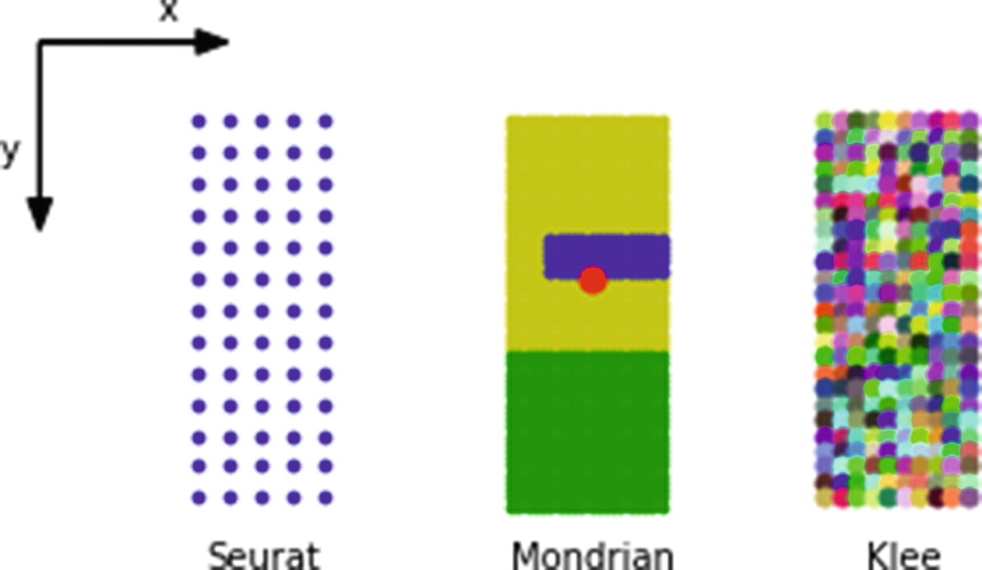
2.2 Dot Art

Interesting patterns can be created by arranging dots in a geometric pattern. Figure 2-4 shows some examples. In all three cases, the dots are arranged in a two-dimensional x,y matrix. You can vary the size of the dots, colors, and the x and y limits of the matrix. Each matrix is created with nested for loops, as shown in Listing 2-2, lines 20-22, 25-­35, and 40-45. These nested loops sweep in the x direction then, at each x, in the y direction, thus filling out a rectangular area. Mondrian is composed of three separate dot rectangles plus a large red dot.
../images/456962_1_En_2_Chapter/456962_1_En_2_Fig4_HTML.jpg
Figure 2-4

Dot art created created by Listing 2-2

In line 7, you import random. This is a library of random functions that you use in lines 42, 43, and 44 to produce random primary r,g,b color components. They are mixed in line 45. You will use random’s random.randrange(a,b,c) function to obtain the random values. You could also use the random functions that are included in numpy, although the syntax is a bit different. The random library is being used here to illustrate that there are other math libraries besides numpy .

random.randrange(a,b,c) returns a random number between a and b in increments c. a, b, and c must be integers. To obtain a wide selection of random numbers, let a=1, b=100, and c=1 in lines 42-44. But rr in line 42 must be between 0 and 1.0 so you divide by 100 in line 42. This provides a random value for rr, the red component of the color mix, between 0 and 1.0. Similarly for rg and rb, the green and blue components, in lines 43 and 44. As you can see, the results in Klee are quite interesting.

1   """
2   DOTART
3   """
4
5   import matplotlib.pyplot as plt
6   import numpy as np
7   import random
8
9   plt.axis([10,140,90,-10])
10
11  plt.axis('off')
12  plt.grid(False)
13
14  plt.arrow(0,0,20,0,head_length=4,head_width=3,color='k')
15  plt.arrow(0,0,0,20,head_length=4,head_width=3,color='k')
16  plt.text(15,-3,'x')
17  plt.text(-5,15,'y')
18
19  #————————————————————————————————————————————-plot Seurat
20  for x in np.arange(20,40,4):
21        for y in np.arange(10,60,4):
22              plt.scatter(x,y,s=8,color='b')
23
24  #————————————————————————————————————————————–plot Mondrian
25  for x in np.arange(60,80,1):
26        for y in np.arange(10,40,1):
27              plt.scatter(x,y,s=8,color='y')
28
29  for x in np.arange(60,80,1):
30        for y in np.arange(40,60):
31              plt.scatter(x,y,s=8,color='g')
32
33  for x in np.arange(65,80,1):
34        for y in np.arange(25,30,1):
35              plt.scatter(x,y,s=8,color='b')
36
37  plt.scatter(70,30,s=50,color='r')
38
39  #————————————————————————————————————————————plot Klee
40  for x in np.arange(100,120,2):
41        for y in np.arange(10,60,2):
42              rr=random.randrange(0,100,1)/100 #–random red 0<=rr<=1
43              rg=random.randrange(0,100,1)/100 #–random green 0<=rg<=1
44              rb=random.randrange(0,100,1)/100 #–random blue 0<=rb<=1
45        plt.scatter(x,y,s=25,color=(rr,rg,rb))
46
47  #————————————————————————————————————————————labels
48  plt.text(105,67,'Klee')
49  plt.text(60,67,'Mondrian')
50  plt.text(21,67,'Seurat')
51
52  plt.show()
Listing 2-2

Program DOTART

2.3 Circular Arcs from Dots

Listing 2-3 draws a circular arc using points. This is your first program dealing with circular coordinates, angles, and trig functions. The geometry used by Listing 2-3 is shown in Figure 2-5. The output is shown in Figure 2-6.

Lines 25-31 in Listing 2-3 plot the arc. The center of curvature is at (xc,yc) as defined in lines 20 and 21. The radius of curvature is r in line 22. The arc starts at point 1, which is at an angle p1 relative to the x axis. It ends at point 2, which is at an angle p2. These angles, 20 and 70 degrees respectively, are set in lines 25 and 26 where they are converted to radians, the units required by np.sin() and np.cos() . In later programs, you will use the radians() function , which converts an argument from degrees to radians. The points on the arc are spaced an angular increment dp apart, as shown in line 27. dp is set to the total angle spanned by the arc, p2-p1, divided by 100. A wider spacing, say (p2-p1)/20, especially when combined with a smaller dot size, will give a more coarse arc. The loop running from line 28 to 31 advances the angle of each point by the increment dp using the arange() function . Lines 29 and 30 calculate the coordinates of each point relative to the global x,y system, which has its origin at (0,0). The global coordinates are those used for plotting. xp=r*np.cos(p) and yp=r*np.(sin(p) are the coordinates of p along the arc relative to the arc’s center of curvature at (xc,yc). These are local coordinates. The coordinates of the center of curvature (xc,yc) must be added to the local coordinates to obtain the global coordinates relative to x=0,y=0. This is done in lines 29 and 30. Line 31 plots a green dot of size 1 at each location using the global coordinates. The results are shown in Figure 2-5 and the code is shown in Listing 2-4.
../images/456962_1_En_2_Chapter/456962_1_En_2_Fig5_HTML.jpg
Figure 2-5

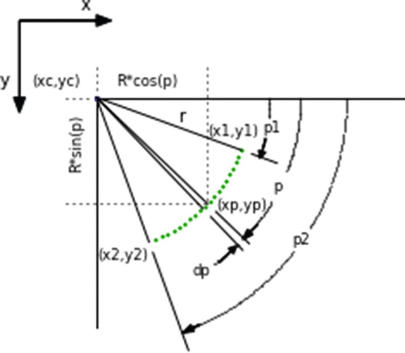
Geometric model used for creating a circular arc with scatter() dots, created by Listing 2-4

../images/456962_1_En_2_Chapter/456962_1_En_2_Fig6_HTML.jpg
Figure 2-6

Circular arc created with np.scatter() dots

1   """
2   PARC
3   """
4
5   import numpy as np
6   import matplotlib.pyplot as plt
7
8   plt.axis([-10,140,90,-10])
9
10  plt.axis('on')
11  plt.grid(True)
12
13  #—————————————————————————————————————————————axes
14  plt.arrow(0,0,20,0,head_length=4,head_width=3,color='k')
15  plt.arrow(0,0,0,20,head_length=4,head_width=3,color='k')
16
17  plt.text(16,-3,'x')
18  plt.text(-5,17,'y')
19
20  xc=20
21  yc=20
22  r=40
23
24  #——————————————————————————————————————————plot arc
25  p1=20*np.pi/180
26  p2=70*np.pi/180
27  dp=(p2-p1)/100
28  for p in np.arange(p1,p2,dp):
29      x=xc+r*np.cos(p)
30      y=yc+r*np.sin(p)
31      plt.scatter(x,y,s=1,color='g')
32
33  #———————————————————————————————————————————labels
34  plt.text(61,34,'(x1,y1)')
35  plt.text(16,60,'(x2,y2)')
36  plt.scatter(xc,yc,s=10,color='k')
37  plt.text(xc+4,yc-4,'(xc,yc)',color='k')
38
39  plt.show()
Listing 2-3

Program PARC

(The following is the program that created Figure 2-5)

1   """
2   PARCGEOMETRY
3   """
4
5   import numpy as np
6   import matplotlib.pyplot as plt
7
8   plt.axis([-10,140,90,-10])
9
10  plt.axis('off')
11  plt.grid(False)
12
13  #—————————————————————————————————————coordinate axes
14  plt.arrow(0,0,20,0,head_length=4,head_width=3,color='k')
15  plt.arrow(0,0,0,20,head_length=4,head_width=3,color='k')
16
17  #———————————————————————————————————————————labels
18  plt.text(16,-3,'x')
19  plt.text(-5,17,'y')
20
21  #———————————————————————————————————————main arc
22  xc=20
23  yc=20
24  r=40
25  plt.scatter(xc,yc,color='b',s=5)
26
27  phi1=20*np.pi/180.
28  phi2=70*np.pi/180.
29  dphi=(phi2-phi1)/20.
30  for phi in np.arange(phi1,phi2,dphi):
31       x=xc+r*np.cos(phi)
32       y=yc+r*np.sin(phi)
33       plt.scatter(x,y,s=2,color='g')
34
35  plt.plot([xc,xc+r*np.cos(phi1)],[yc,yc+r*np.sin(phi1)],color='k')
36
37  x1=xc+(r+3)*np.cos(phi1)
38  x2=xc+(r+10)*np.cos(phi1)
39  y1=yc+(r+3)*np.sin(phi1)
40  y2=yc+(r+10)*np.sin(phi1)
41  plt.plot([x1,x2],[y1,y2],color='k')
42
43  x1=xc+(r+3)*np.cos(phi2)
44  x2=xc+(r+30)*np.cos(phi2)
45  y1=yc+(r+3)*np.sin(phi2)
46  y2=yc+(r+30)*np.sin(phi2)
47  plt.plot([x1,x2],[y1,y2],color='k')
48
49  plt.plot([xc,xc+r*np.cos(phi2)],[yc,yc+r*np.sin(phi2)],color='k')
50
51  phihalf=(phi1+phi2)*.5
52  phi3=phihalf-dphi/2
53  phi4=phihalf+dphi/2
54
55  plt.plot([xc,xc+r*np.cos(phi3)],[yc,yc+r*np.sin(phi3)],color='k')
56  plt.plot([xc,xc+r*np.cos(phi4)],[yc,yc+r*np.sin(phi4)],color='k')
57
58  x1=xc+(r+3)*np.cos(phi3)
59  x2=xc+(r+15)*np.cos(phi3)
60  y1=yc+(r+3)*np.sin(phi3)
61  y2=yc+(r+15)*np.sin(phi3)
62  plt.plot([x1,x2],[y1,y2],color='k')
63
64  x1=xc+(r+3)*np.cos(phi4)
65  x2=xc+(r+15)*np.cos(phi4)
66  y1=yc+(r+3)*np.sin(phi4)
67  y2=yc+(r+15)*np.sin(phi4)
68  plt.plot([x1,x2],[y1,y2],color='k')
69
70  #———————————————————————————————————————————P1 arc
71  dphi=(phi3)/100.
72  for phi in np.arange(0,phi1/2-3.2*np.pi/180,dphi):
73       x=xc+(r+5)*np.cos(phi)
74       y=yc+(r+5)*np.sin(phi)
75       plt.scatter(x,y,s=.1,color='k')
76
77  for phi in np.arange(phi1/2+3.3*np.pi/180,phi1,dphi):
78       x=xc+(r+5)*np.cos(phi)
79       y=yc+(r+5)*np.sin(phi)
80       plt.scatter(x,y,s=.1,color='k')
81
82  #————————————————————————————————————————————P2 arc
83  dphi=(phi3)/100.
84  for phi in np.arange(0,phi2/2-3.2*np.pi/180,dphi):
85       x=xc+(r+25)*np.cos(phi)
86       y=yc+(r+25)*np.sin(phi)
87       plt.scatter(x,y,s=.1,color='k')
88
89  dphi=(phi3)/100.
90  for phi in np.arange(phi2/2+3.2*np.pi/180,phi2,dphi):
91       x=xc+(r+25)*np.cos(phi)
92       y=yc+(r+25)*np.sin(phi)
93       plt.scatter(x,y,s=.1,color='k')
94
95  #————————————————————————————————————————————P arc
96  dphi=(phi3)/100.
97  for phi in np.arange(0,phi3/2-.5*np.pi/180,dphi):
98       x=xc+(r+13)*np.cos(phi)
99       y=yc+(r+13)*np.sin(phi)
100      plt.scatter(x,y,s=.1,color='k')
101
102 dphi=(phi3)/100.
103 for phi in np.arange(phi3/2+9.*np.pi/180,phi3,dphi):
104      x=xc+(r+13)*np.cos(phi)
105      y=yc+(r+13)*np.sin(phi)
106      plt.scatter(x,y,s=.1,color='k')
107
108 #————————————————————————————————————————dp arc
109 dphi=(phi3)/100.
110 for phi in np.arange(phi3+5*dphi,phi3+25*dphi,dphi):
111      x=xc+(r+13)*np.cos(phi)
112      y=yc+(r+13)*np.sin(phi)
113      plt.scatter(x,y,s=.1,color='k')
114
115 plt.plot([xc,100],[yc,yc],'k')
116 plt.plot([xc,xc],[yc,80],'k')
117
118 #————————————————————————————————————————labels
119 plt.text(71,58,'p2',size='small')
120 plt.text(66,44,'p',size='small')
121 plt.text(63,29,'p1',size='small')
122 plt.text(45,66,'dp',size='small')
123 plt.text(41,26,'r')
124 plt.text(3,17,'(xc,yc)',size='small')
125 plt.plot([xc+r*np.cos(phi3),xc+r*np.cos(phi3)],[yc-8,yc+r*np.sin(phi3)],'k:')
126 plt.plot([xc,xc],[yc-2,yc-8],'k:')
127 plt.text(25,17,'R*cos(p)',size='small')
128
129 plt.plot([xc-8,xc+r*np.cos(phi3)],[yc+r*np.sin(phi3),yc+r*np.sin(phi3)],'k:')
130 plt.plot([xc-2,xc-8],[yc,yc],'k:')
131 plt.text(13,27,'R*sin(p)',size='small',rotation=90)
132
133 plt.text(49,30,'(x1,y1)',size='small')
134 plt.text(20,62,'(x2,y2)',size='small')
135 plt.text(51,49,'(xp,yp)',size='small')
136
137 #——————————————————————————————————————————arrow heads
138 plt.arrow(47,79,-2,1,head_length=3,head_width=2,color='k')
139 plt.arrow(62,53,-2,2,head_length=2.9,head_width=2,color='k')
140 plt.arrow(64,31,-.9,3,head_length=2,head_width=2,color='k')
141 plt.arrow(52,63,3,-3,head_length=2,head_width=2,color='k')
142
143 plt.show()
Listing 2-4

Program PARCGEOMETRY

2.4 Circular Arcs from Line Segments

Instead of plotting dots with np.scatter() at points along the arc, you can create a finer arc using straight-line segments between points. If you replace the “plot arc” routine in Listing 2-3, beginning at line 24, with

24  #—————————————————————————————————plot arc
25  p1=20*np.pi/180
26  p2=70*np.pi/180
27  dp=(p2-p1)/100
28  xlast=xc+r*np.cos(p1)
29  ylast=yc+r*np.sin(p1)
30  for p in np.arange(p1+dp,p2,dp):
31        x=xc+r*np.cos(p)
32        y=yc+r*np.sin(p)
33        plt.plot([xlast,x],[ylast,y],color='g')
34        xlast=x
35        ylast=y

you get the arc shown in Figure 2-7. In lines 28 and 29 of the code above you define xlast and ylast. These are the last x and y coordinate values plotted at the end of the previous line segment. Since you are just starting to plot the arc before the loop begins, these are initially set equal to the arc’s starting point where p=p1. You will need them to plot the first arc segment in line 33. Parameters p, p1, p2, and dp are the same as before. Imagine the loop 30-35 is just starting to run. Lines 31 and 32 calculate the global coordinates of the end of the first line segment, which is dp into the arc. Using the previously set values xlast and ylast, which are the coordinates of the beginning of that line segment in 28 and 29, line 33 plots the first line segment. Lines 34 and 35 update the end coordinates of the first segment as xlast, ylast. These will be used as the beginning coordinates of the second line segment. The loop continues to the end of the arc using the end of the preceding segment as the beginning of the next one. Notice in line 30 the loop begins at p1+dp, the end angle of the first line segment. This isn’t actually necessary and the beginning of the loop could be set to p1 as before, in which case the first line segment would have zero length. The loop would continue to the end of the arc as before.

../images/456962_1_En_2_Chapter/456962_1_En_2_Fig7_HTML.jpg
Figure 2-7

Circular arc created with plt.plot() line segments

In future work, you will sometimes use curves constructed of dots instead of line segments. Even though dots do not produce as fine results, they avoid complicating the plotting algorithm, which can sometimes obscure the logic of the script. However, line segments do produce superior results so you will use them as well.

2.5 Circles

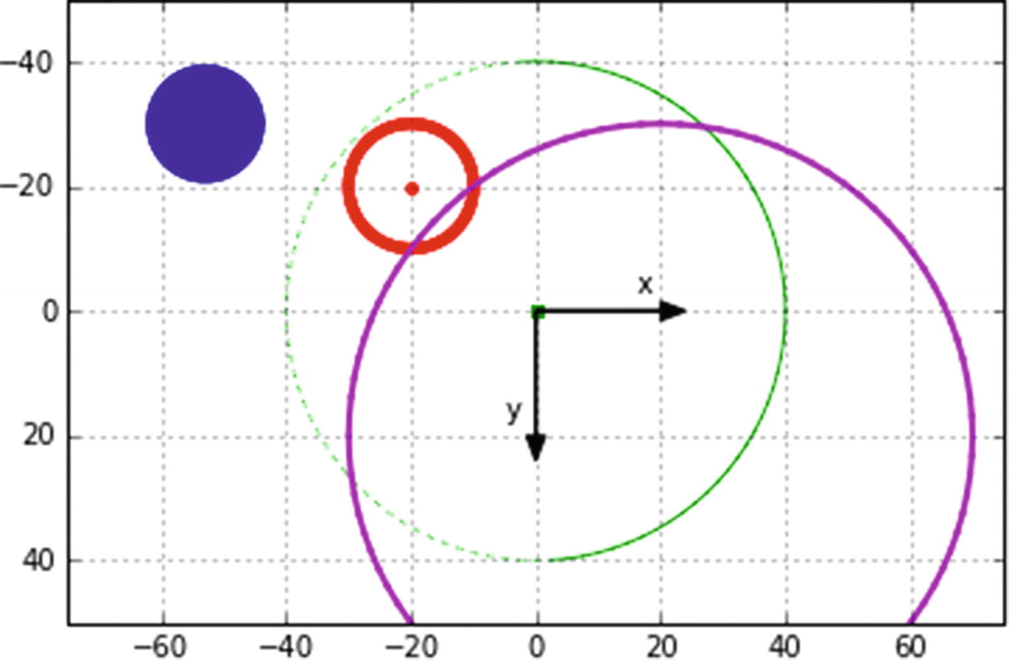
A full circle is just a 360 ° arc. You can make a full circle by changing the beginning and end angles of the arc in the previous section to p1=0 and p2=360 degrees. This is done in lines 24 and 25 of Listing 2-5. The output is shown in Figure 2-8. Three circles and a solid disc are plotted at different locations. They have different colors and widths. Half the green circle is plotted with solid-line segments, the other half with dashed lines 29-37. The decision to plot a solid or dashed line is made by the if logic between lines 32 and 35. This changes the linestyle attribute in line 33. The blue solid disc is made by plotting concentric circles with radii from r1=0 to the disc’s outer radius r2. You could, of course, also make a solid disk with the np.scatter() function . You should be able to follow the logic used here to create the various circles by examining the script in Listing 2-5.

This program could have been shortened by the use of functions. It has been left open for the sake of clarity by using cut and paste to reproduce sections of redundant code.

1   """
2   CIRCLES
3   """
4
5   import numpy as np
6   import matplotlib.pyplot as plt
7
8   plt.axis([-75,75,50,-50])
9
10  plt.axis('on')
11  plt.grid(True)
12
13  plt.arrow(0,0,20,0,head_length=4,head_width=3,color='k')
14  plt.arrow(0,0,0,20,head_length=4,head_width=3,color='k')
15
16  plt.text(16,-3,'x')
17  plt.text(-5,17,'y')
18
19  #——————————————————————————————————–green circle
20  xc=0
21  yc=0
22  r=40
23
24  p1=0*np.pi/180
25  p2=360*np.pi/180
26  dp=(p2-p1)/100
27  xlast=xc+r*np.cos(p1)
28  ylast=yc+r*np.sin(p1)
29  for p in np.arange(p1,p2+dp,dp):
30        x=xc+r*np.cos(p)
31        y=yc+r*np.sin(p)
32        if p > 90*np.pi/180 and p < 270*np.pi/180:
33             plt.plot([xlast,x],[ylast,y],color='g',linestyle=':')
34        else:
35             plt.plot([xlast,x],[ylast,y],color='g')
36        xlast=x
37        ylast=y
38
39  plt.scatter(xc,yc,s=15,color='g')
40
41  #————————————————————————————————————————red circle
42  xc=-20
43  yc=-20
44  r=10
45
46  p1=0*np.pi/180
47  p2=360*np.pi/180
48  dp=(p2-p1)/100
49  xlast=xc+r*np.cos(p1)
50  ylast=yc+r*np.sin(p1)
51  for p in np.arange(p1,p2+dp,dp):
52        x=xc+r*np.cos(p)
53        y=yc+r*np.sin(p)
54        plt.plot([xlast,x],[ylast,y],linewidth=4,color='r')
55        xlast=x
56        ylast=y
57
58  plt.scatter(xc,yc,s=15,color='r')
59
60  #—————————————————————————————————————————purple circle
61  xc=20
62  yc=20
63  r=50
64
65  p1=0*np.pi/180
66  p2=360*np.pi/180
67  dp=(p2-p1)/100
68  xlast=xc+r*np.cos(p1)
69  ylast=yc+r*np.sin(p1)
70  for p in np.arange(p1,p2+dp,dp):
71        x=xc+r*np.cos(p)
72        y=yc+r*np.sin(p)
73        plt.plot([xlast,x],[ylast,y],linewidth=2,color=(.8,0,.8))
74        xlast=x
75        ylast=y
76
77  plt.scatter(xc,yc,color=(.5,0,.5))
78
79  #———————————————————————————————————————————blue disc
80  xc=-53
81  yc=-30
82  r1=0
83  r2=10
84  dr=1
85
86  p1=0*np.pi/180
87  p2=360*np.pi/180
88  dp=(p2-p1)/100
89  xlast=xc+r1*np.cos(p1)
90  ylast=yc+r1*np.sin(p1)
91  for r in np.arange(r1,r2,dr):
92        for p in np.arange(p1,p2+dp,dp):
93              x=xc+r*np.cos(p)
94              y=yc+r*np.sin(p)
95              plt.plot([xlast,x],[ylast,y],linewidth=2,color=(0,0,.8))
96              xlast=x
97              ylast=y
98
99  plt.show()
Listing 2-5

Program CIRCLES

../images/456962_1_En_2_Chapter/456962_1_En_2_Fig8_HTML.jpg
Figure 2-8

Circles created by Listing 2-5

2.6 Dot Discs

Two discs created with different dot patterns are shown in Figure 2-9. The disc labelled “r,p” is drawn by placing dots in a traditional polar r,p array where r is the radius from the center and p is the angle. The algorithm starts at line 21 in Listing 2-6. The script in Listing 2-6 should be self-explanatory. The only issue with this plot is that the dots are not uniformly spaced but are further apart as the radius increases. This may be undesirable in some situations.
../images/456962_1_En_2_Chapter/456962_1_En_2_Fig9_HTML.jpg
Figure 2-9

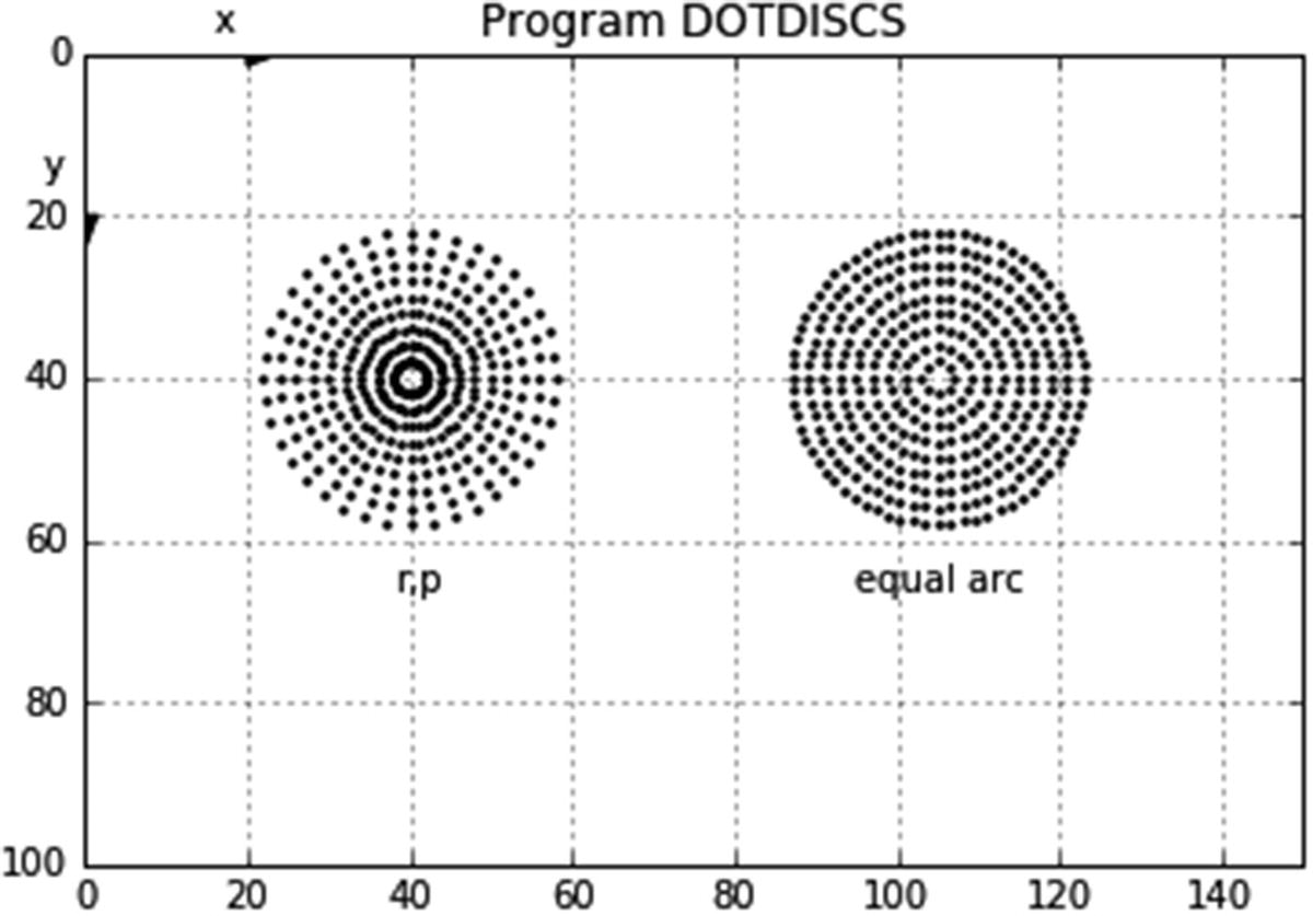
Discs created by different dot patterns in Listing 2-6 where “r,p” contains simple polar coordinates and “equal arc” has modified polar coordinates

The “equal arc” disc, beginning in line 38, appears better visually. As with the “r,p” disc, the dots are equally spaced in the radial direction. However, in the “equal arc” disc, the number of dots in the circumferential direction at each radial location becomes larger as the radius increases, thus keeping the circumferential arc spacing between dots constant. The model used is shown in Figure 2-10. dc is the circumferential spacing between dots a and b at rmax, the outer edge of the disk. dp is the angular spacing between radii to a and b. To achieve more uniform spacing across the disc, you hold dc constant at all radii. A typical radial location is shown at r=rmax/2. dc at this radius is the same as at rmax and is equal to dc. To accommodate this spacing, the angle between adjacent dots must increase to drp.

In line 44 of Listing 2-6, the disc’s outer radius is set to 20. The radial spacing is set to 2 in line 45. Keeping in mind that the circumferential spacing between two points on a circular arc is r×dp where r is the radius and dp is the angle between the points, line 46 calculates dc where you have arbitrarily set the number of dots at rmax to 40 per π radians (80 around the complete circumference). The loop beginning at line 48 starts at r=dr and advances in the radial direction to rmax in steps dr. At each value or r, the angle between dots dpr required to keep the circumferential spacing equal to dc is calculated in line 49. The loop beginning at line 50 then places the dots circumferentially.
../images/456962_1_En_2_Chapter/456962_1_En_2_Fig10_HTML.jpg
Figure 2-10

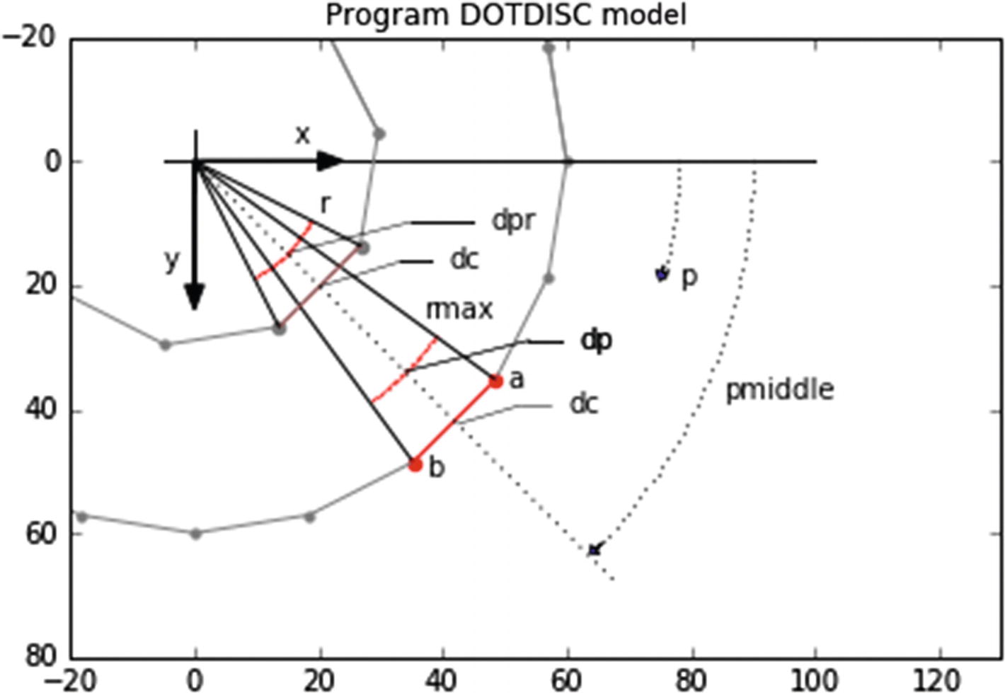
Model for “equal arc” disc used by Listing 2-6

1   """
2   DOTDISCS
3   """
4
5   import matplotlib.pyplot as plt
6   import numpy as np
7   import random as rnd
8
9   plt.axis([0,150,100,0])
10
11  plt.axis('off')
12  plt.grid(False)
13
14  plt.arrow(0,0,20,0,head_length=4,head_width=3,color='k')
15  plt.arrow(0,0,0,20,head_length=4,head_width=3,color='k')
16
17  plt.text(16,-3,'x')
18  plt.text(-5,17,'y')
19
20  #—————————————————————————————————————————simple r,p dot pattern
21  xc=40
22  yc=25
23
24  p1=0
25  p2=2*np.pi
26  dp=np.pi/20
27
28  rmax=20
29  dr=2
30
31  for r in np.arange(dr,rmax,dr):
32        for p in np.arange(p1,p2,dp):
33              x=xc+r*np.cos(p)
34              y=yc+r*np.sin(p)
35              plt.scatter(x,y,s=2,color='k')
36
37  #—————————————————————————————————————————equal arc length dot pattern
38  xc=40
39  yc=70
40
41  p1=0
42  p2=2*np.pi
43
44  rmax=20
45  dr=2
46  dc=np.pi*rmax/40
47
48  for r in np.arange(dr,rmax,dr):
49       dpr=dc/r
50       for p in np.arange(p1,p2,dpr):
51            x=xc+r*np.cos(p)
52            y=yc+r*np.sin(p)
53            plt.scatter(x,y,s=2,color='k')
54
55  #————————————————————————————————————————————————————labels
56  plt.text(38,66,'r,p')
57  plt.text(95,66,'equal arc')
58
59  plt.show()
Listing 2-6

Program DOTDISCS

2.7 Ellipses

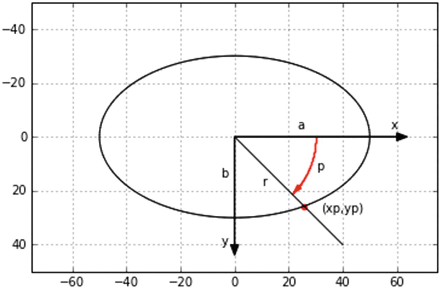
Ellipses are shown in Figure 2-12. They were drawn by Listing 2-7. The model used by Listing 2-7 is shown in Figure 2-11. This was drawn by Listing 2-8. The dimension a is called the semi-major since it refers to half the greater width; b is the semi-minor. 2a and 2b are the major and minor dimensions .

The equation of an ellipse, which we are all familiar with, is,
$$ frac{x^2}{a^2}+frac{y^2}{b^2}=1 $$
(2-7)
In the special case where a=b=r, this degenerates to a circle, as in
$$ {x}^2+{y}^2={r}^2 $$
(2-8)
where r is the radius.
A possible strategy to use when plotting an ellipse is to start at x=-a and advance in the +x direction using Equation 2-7 to calculate y at each x, and then plot either a dot or a line segment from the last step, as you have done in the past. The y coordinate is easily derived from Equation 2-7 as
$$ y=bsqrt{1-frac{x^2}{a^2}} $$
(2-9)

This seems easy enough. The green ellipse in Figure 2-12 was drawn this way. However, there is a problem. Look at Listing 2-7, lines 48, 49, and 50; the square root in Equation 2-9 and in line 48 gives uncertain results as x approaches +a and line 48 tries to take the square root of a number very close to zero. This is caused by roundoff errors in Python’s calculations. The manifestation of this shows up as a gap at the +a side of the ellipse. In the algorithm for the green ellipse, this gap is closed by lines 54 and 55. You can get a decent ellipse this way but you have to be careful.

Another way is to use polar coordinates , as shown in Figure 2-11. You want to determine the coordinates (xp,yp) for a point on the ellipse as a function of the angle p. By varying p, you will have the information you need to plot the ellipse. To determine (xp,yp) vs. p, you note that it lies on the intersection of the ellipse and the radial line. This point is indicated by the red dot. Incidentally, the dot does not appear to lie exactly at the intersection, as can be seen. This is because the scale factor used to adjust the x axis values in line 8 of Listing 2-8 is a bit off. You used a rough measurement with a ruler and then you rounded off the results of the calculation to determine the scale factor. The resulting slight errors are showing up here. The equation of the line can be determined from the following:
$$ xp=r; cos(p) $$
(2-10)
$$ yp=r; sin(p) $$
(2-11)
Combining the above,
$$ frac{yp}{xp}=frac{r; sin(p)}{r; cos(p)}= tan(p) $$
(2-12)
$$ yp=xp; tan(p) $$
(2-13)
You know that (xp,yp) lies at the intersection of the line and the ellipse. This is where the equations for both the line and the ellipse are satisfied by xp and yp. You can determine the coordinates of this point by substituting Equation 2-13 into Equation 2-7,
$$ frac{x{p}^2}{a^2}+frac{x{p}^2ta{n}^2p}{b^2}=1 $$
(2-14)
which works out to
$$ xp= ab{left[{b}^2+{a}^2ta{n}^2(p)
ight]}^{-frac{1}{2}} $$
(2-15)
$$ yp= ab{left[{a}^2+{b}^2frac{1}{ta{n}^2(p)}
ight]}^{-frac{1}{2}} $$
(2-16)
../images/456962_1_En_2_Chapter/456962_1_En_2_Fig11_HTML.jpg
Figure 2-11

Model created by Listing 2-8 and used by Listing 2-7

Equations 2-15 and 2-16 are implemented in Listing 2-7 to draw the red ellipse between lines 20 and 36, the green ellipse between lines 39 and 55, and the blue ellipse in lines 58 and 69. The output is shown in Figure 2-12. When drawing the green ellipse, the program loops from -a to +a and uses Equation 2-9 to calculate y values. As mentioned, this can lead to roundoff errors near the extremity of the ellipse at x=+a, which leaves a gap in the ellipse. This is corrected in lines 54 and 55, which draw short lines to close the gap. Note that the blue ellipse is filled in. This is accomplished by line 69, which plots vertical lines from the top to the bottom of the ellipse.
../images/456962_1_En_2_Chapter/456962_1_En_2_Fig12_HTML.jpg
Figure 2-12

Ellipses created by Listing 2-7

1   """
2   ELLIPSES
3   """
4
5   import numpy as np
6   import matplotlib.pyplot as plt
7
8   plt.axis([-75,75,50,-50])
9
10  plt.axis('on')
11  plt.grid(True)
12
13  plt.arrow(0,0,60,0,head_length=4,head_width=3,color='k')
14  plt.arrow(0,0,0,45,head_length=4,head_width=3,color='k')
15
16  plt.text(58,-3,'x')
17  plt.text(-5,44,'y')
18
19  #————————————————————————————————————————red ellipse
20  a=40
21  b=20.
22  p1=0
23  p2=180*np.pi/180
24  dp=.2*np.pi/180
25
26  xplast=a
27  yplast=0
28  for p in np.arange(p1,p2,dp):
29          xp=np.abs(a*b*(b*b+a*a*(np.tan(p))**2.)**-.5)
30          yp=np.abs(a*b*(a*a+b*b/(np.tan(p)**2.))**-.5)
31          if p > np.pi/2:
32               xp=-xp
33          plt.plot([xplast,xp],[yplast,yp],color='r')
34          plt.plot([xplast,xp],[-yplast,-yp],color='r')
35          xplast=xp
36          yplast=yp
37
38  #————————————————————————————————————————green ellipse
39  a=20.
40  b=40.
41  xp1=-a
42  xp2=a
43  dx=.1
44
45  xplast=-a
46  yplast=0
47  for xp in np.arange(xp1,xp2,dx):
48       yp=b*(1-xp**2./a**2.)**.5
49       plt.plot([xplast,xp],[yplast,yp],linewidth=1,color='g')
50       plt.plot([xplast,xp],[-yplast,-yp],linewidth=1,color='g')
51       xplast=xp
52       yplast=yp
53
54  plt.plot([xplast,a],[yplast,0],linewidth=1,color='g'
55  plt.plot([xplast,a],[-yplast,0],linewidth=1,color='g'
56
57  #—————————————————————————————————————blue ellipse
58  a=5.
59  b=15.
60  p1=0
61  p2=180*np.pi/180
62  dp=.2*np.pi/180
63
64  for p in np.arange(p1,p2,dp):
65        xp=np.abs(a*b*(b*b+a*a*(np.tan(p))**2.)**-.5)
66        yp=np.abs(a*b*(a*a+b*b/(np.tan(p)**2.))**-.5)
67        if p > np.pi/2:
68             xp=-xp
69        plt.plot([xp,xp],[yp,-yp],linewidth=1,color='b')
70
71  plt.show()
Listing 2-7

Program ELLIPSES

(The following program was used to create Figure 2-11.)

1   """
2   ELLIPSEMODEL
3   """
4
5   import numpy as np
6   import matplotlib.pyplot as plt
7
8   plt.axis([-75,75,50,-50])
9
10  plt.axis('on')
11  plt.grid(True)
12
13  plt.arrow(0,0,60,0,head_length=4,head_width=3,color='k')
14  plt.arrow(0,0,0,40,head_length=4,head_width=3,color='k')
15
16  plt.text(58,-3,'x')
17  plt.text(-5,40,'y')
18
19  #——————————————————————————————————————ellipse
20  a=50.
21  b=30.
22  p1=0.
23  p2=180.*np.pi/180.
24  dp=(p2-p1)/180.
25
26  xplast=a
27  yplast=0
28  for p in np.arange(p1,p2+dp,dp):
29        xp=np.abs(a*b*(b*b+a*a*(np.tan(p))**2.)**-.5)
30        yp=np.abs(a*b*(a*a+b*b/(np.tan(p)**2.))**-.5)
31        if p > np.pi/2:
32             xp=-xp
33        plt.plot([xplast,xp],[yplast,yp],color='k')
34        plt.plot([xplast,xp],[-yplast,-yp],color='k')
35        xplast=xp
36        yplast=yp
37
38  #———————————————————————————————————————————line
39  plt.plot([0,40],[0,40],color='k')
40
41  #———————————————————————————————————————————point
42  p=45.*np.pi/180.
43  xp=np.abs(a*b*(b*b+a*a*(np.tan(p))**2.)**-.5)
44  yp=np.abs(a*b*(a*a+b*b/(np.tan(p)**2.))**-.5)
45  plt.scatter(xp,yp,s=20,color='r')
46
47  #—————————————————————————————————————————labels
48  plt.text(23,-3,'a',color='k')
49  plt.text(-5,15,'b',color='k')
50  plt.text(32,28,'(xp,yp)')
51  plt.text(30,12,'p')
52  plt.text(10,18,'r')
53
54  #——————————————————————————————————————————p arc
55  p1=0
56  p2=45*np.pi/180
57  dp=(p2-p1)/180
58  r=30
59  for p in np.arange(p1,p2,dp):
60        x=r*np.cos(p)
61        y=r*np.sin(p)
62        plt.scatter(x,y,s=.1,color='r')
63
64  plt.arrow(25,17.5,-1,1,head_length=3,head_width=2,color='r')
65
66  plt.show()
Listing 2-8

Program ELLIPSEMODEL

2.8 2D Translation

In two dimensions, an object has three independent degrees of freedom: it can rotate around one axis direction which is perpendicular to the plane and it can translate in two directions (x and y) within the plane. Pure translation implies the object is moved without rotation; pure rotation implies the object is rotated without translation. The objects in Figure 2-13 are examples of pure translation. The triangle (black) has been translated (moved) to the right (green) without rotation and then down (red). This is a simple thing to accomplish with Python, especially when using lists as in Listing 2-9. For example, to move an object to the right in an amount of dx, just add dx to the x coordinates and replot it. Similarly for the y direction, just add dy to the y coordinates and replot. The small blue boxes were translated across the plotting area by incrementing the x coordinates by 10 units in the loop beginning in line 45.
../images/456962_1_En_2_Chapter/456962_1_En_2_Fig13_HTML.jpg
Figure 2-13

Examples of translation created by Listing 2-9

1   """
2   2DTRANSLATION
3   """
4
5   import numpy as np
6   import matplotlib.pyplot as plt
7
8   x1=-10
9   x2=140
10  y1=90
11  y2=-10
12  plt.axis([x1,x2,y1,y2])
13
14  plt.axis('on')
15  plt.grid(True)
16
17  plt.title('Translation')
18
19  #—————————————————————————————————————————————————triangle
20  x=[20,30,40,20]
21  y=[40,20,40,40]
22  plt.plot(x,y,color='k')
23  plt.plot(x,y,color='k')
24  plt.plot(x,y,color='k')
25
26  #——————————————————————————————————————translate triangle dx=60
27  x=[60,70,80,60]
28  plt.plot(x,y,color='g')
29  plt.plot(x,y,color='g')
30  plt.plot(x,y,color='g')
31
32  #——————————————————————————————————————translate triangle dy=40
33  y=[80,60,80,80]
34  plt.plot(x,y,color='r')
35  plt.plot(x,y,color='r')
36  plt.plot(x,y,color='r')
37
38  #——————————————————————————————————————————————————————box
39  x=[0,0,5,5,0]
40  y=[55,50,50,55,55]
41  plt.plot(x,y,'b')
42
43  #————————————————————————————————————————————translate box
44  y=[55,50,50,55,55]
45  for x in np.arange(0,130,10):
46       x=[x,x,x+5,x+5,x]
47       plt.plot(x,y,'b')
48
49  plt.show()
Listing 2-9

Program 2DTRANSLATION

2.9 2D Rotation

So far in this chapter, you have seen how to construct images on a two-dimensional plane using points and lines. In this section, you’ll learn how to rotate a two-dimensional planar object within its own plane. A 2D object that you might want to rotate, a rectangle for example, or something more complicated which will normally consist of any number of points and lines. Lines, of course, are defined by their end points or a series of points if constructed from dots. As you have seen, curves can also be constructed from line segments or dots. If you can determine how to rotate a point, you will then be able to rotate any planar object defined by points. In Chapter 3, you will extend these concepts to the rotation of three-dimensional objects around three coordinate directions.
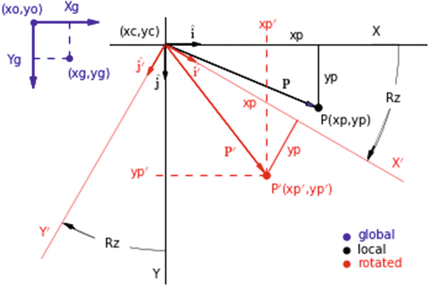
Figure 2-14 shows three coordinate systems: the blue xg,yg system is the global coordinate system . Its numerical size and the location of the global origin (xg=0, yg=0) are defined by the values in the plt.axis([x1,x2,y1,y2]) statement. This is the system you use when plotting. All plotting coordinates should relate to this system. For example, if writing plt.scatter(xg,yg), xg and yg should be relative to the blue xg,yg system as shown.
../images/456962_1_En_2_Chapter/456962_1_En_2_Fig14_HTML.jpg
Figure 2-14

2D rotation model

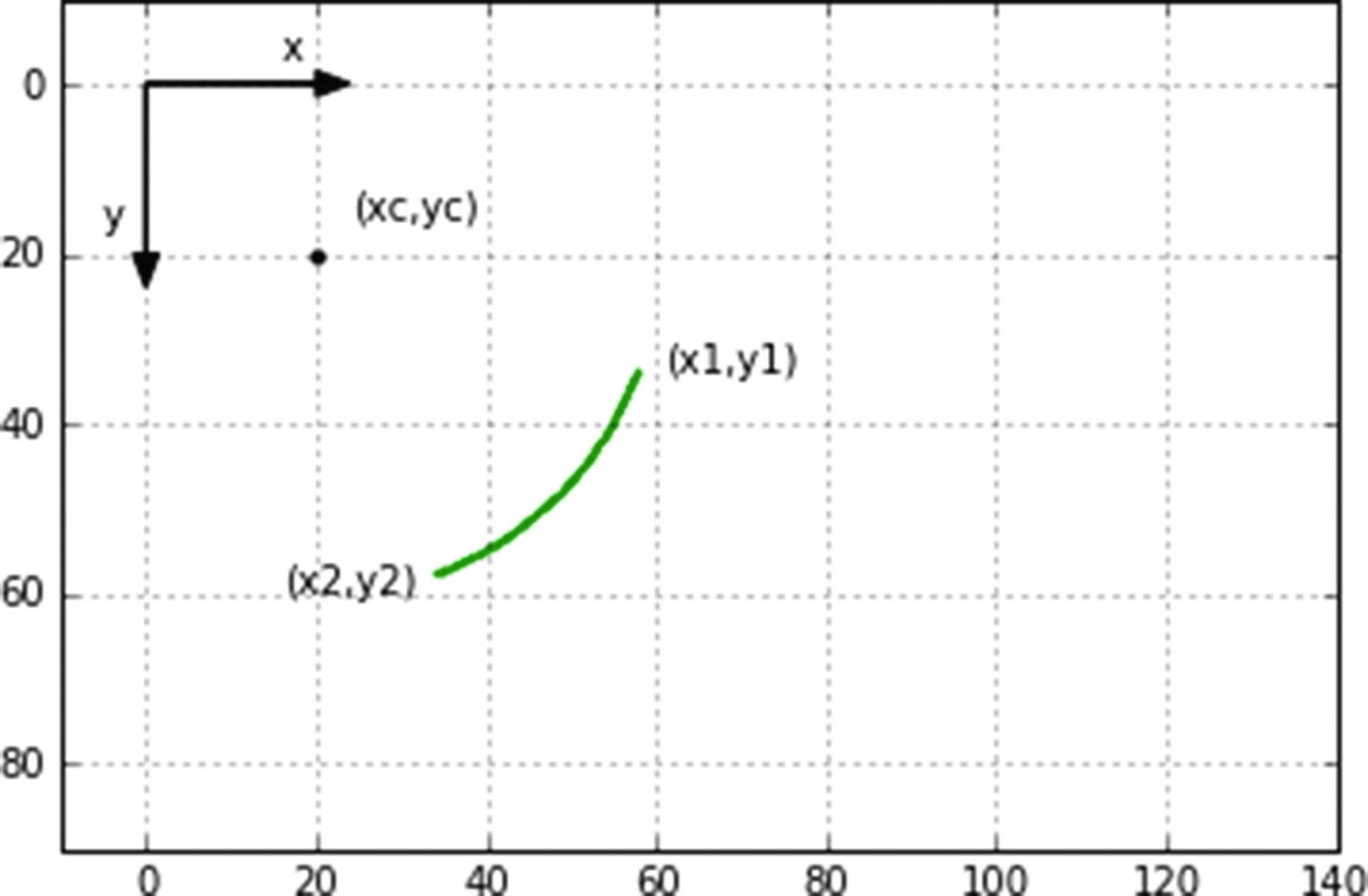
The black x,y system is the local system . A position (xp,yp) in the local system is equivalent to (xc+xp, yc+yp) in the global system. You use the local system to construct shapes by specifying the coordinates of the points that comprise them. For example, if you want to plot a circle somewhere in the plotting area, you could place (xc,yc) at the circle’s center, calculate the points defining the circle around it in reference to the local (black) system, and then relate them back to the xg,yg (blue) system for plotting by translating each point by xc and yc.

Figure 2-14 shows a point P that is rotated through a clockwise angle Rz to a new position at P′. The red coordinate system rotates through the angle Rz. P rotates along with it. The coordinates of P′ in the rotated system, (xp,yp), are the same as they were in the local system. However, in the global system, they are obviously different. Your goal now is to determine the coordinates of P′ in the local system and then in the global system, so you can plot it.

I am using the terminology Rz for the angle because a clockwise rotation in the x,y plane is actually a rotation about the z direction, which points into the plane of the paper. This was illustrated in Chapter 1. It will be explained in more detail in Chapter 3.

Figure 2-14 shows point P in its unrotated position. Its coordinates in relation to the local x,y system (black) are (xp,yp). Its location is defined by the vector P,
$$ mathbf{P}=xpwidehat{mathbf{i}}+ypwidehat{mathbf{j}} $$
(2-17)
where and are unit vectors in the x and y directions.
After P is rotated through the angle Rz, it reaches a new position P′ (red) at coordinates (x′,y′) in relation to the x,y (black) system. P′ is defined by the vector P′ (red) as,
$$ {mathbf{P}}^{mathbf{prime}}=x{p}^{mathit{prime}}widehat{mathbf{i}}+y{p}^{mathit{prime}}widehat{mathbf{j}} $$
(2-18)
The coordinates of P′ in relation to the rotated x′,y′ system are (xp,yp). The position of P′ is thus also defined by the vector
$$ {mathbf{P}}^{mathbf{prime}}=xp{widehat{mathbf{i}}}^{mathbf{prime}}+yp{widehat{mathbf{j}}}^{mathbf{prime}} $$
(2-19)
where ′ and ′ are unit vectors in the x′ and y′ directions.

Your task now is to determine relations for ′ and ′ in relation to and and then substitute them into Equation 2-19. This will give you the coordinates of P′ in relation to the local x,y system. By simply adding xc and yc you will then get the coordinates of P′ in the global system, which you need for plotting.

Four unit vectors are shown at (xc,yc). and point in the x and y directions; ′ and ′ point in the x′ and y′ directions. By examining Figure 2-14, you can see that
$$ {widehat{mathbf{i}}}^{mathbf{prime}}=underset{X; component}{underbrace{cos(Rz)}}kern0.24em widehat{mathbf{i}}+underset{Y; component}{underbrace{sin(Rz)}}kern0.24em widehat{mathbf{j}} $$
(2-20)
$$ {widehat{mathbf{j}}}^{mathbf{prime}}=underset{X; component}{underbrace{mathit{hbox{-}} sin(Rz)}}kern0.24em widehat{mathbf{i}}+underset{Y; component}{underbrace{cos(Rz)}}kern0.24em widehat{mathbf{j}} $$
(2-21)
Plugging these into Equation 2-19, you get
$$ mathbf{p}mathbf{hbox{'}}=xpleft[ cos(Rz)widehat{mathbf{i}}+ sin(Rz)widehat{mathbf{j}}
ight]+ypleft[- sin(Rz)widehat{mathbf{i}}+ cos(Rz)widehat{mathbf{j}}
ight] $$
(2-22)
This can be separated into x and y components ,
$$ {mathbf{P}}^{mathbf{prime}}=x{p}^{mathit{prime}}widehat{mathbf{i}}+y{p}^{mathit{prime}}widehat{mathbf{j}} $$
(2-23)
where
$$ x{p}^{mathit{prime}}=xpleft[ cos(Rz)
ight]+ypleft[- sin(Rz)
ight] $$
(2-24)
$$ y{p}^{mathit{prime}}=xpleft[ sin(Rz)
ight]+ypleft[ cos(Rz)
ight] $$
(2-25)

These last two equations are all you need to rotate a point from (xp,yp) through the angle Rz to new coordinates (xp′,yp′). Note that both sets of coordinates, (xp,yp) and (xp′,yp′), are in reference to the local x,y axes. They can then be easily translated by xc and yc to get them in the global system for plotting.

In the special case where yp=0, that is when P, before rotation, lies on the x axis at x=xp, Equations 2-24 and 2-25 degenerate to
$$ x{p}^{mathit{prime}}=xp; cos(Rz) $$
(2-26)
$$ y{p}^{mathit{prime}}=xp; sin(Rz) $$
(2-27)
which can be easily verified from Figure 2-14. You are, of course, concerned with rotating a generic point that initially is anywhere in the x,y plane so you need the full formulation contained in Equations 2-24 and 2-25. These can be expressed in matrix form as
$$ left[egin{array}{c}hfill x{p}^{mathit{prime}}hfill \ {}hfill y{p}^{mathit{prime}}hfill end{array}
ight]=left[egin{array}{cc}hfill cos(Rz)hfill &amp; hfill mathit{hbox{-}} sin(Rz)hfill \ {}hfill sin(Rz)hfill &amp; hfill cos(Rz)hfill end{array}
ight]left[egin{array}{c}hfill xphfill \ {}hfill yphfill end{array}
ight] $$
(2-28)
which can be abbreviated as
$$ left[{P}^{mathit{prime}}
ight]=left[Rz
ight]left[P
ight] $$
(2-29)
The [P′] and [P] matrices are often termed column vectors since they contain the components of vectors P and P′. [Rz] is a transformation matrix; it transforms the P vector into the P′ vector, in this case by rotation through the angle Rz. These vectors are shown in Figure 2-15 where P defines the location of the unrotated point P1 (black) and the rotated point P′ (red) at P3. You can rewrite [Rz] as
$$ left[Rz
ight]=left[egin{array}{cc}hfill Cleft(1,1
ight)hfill &amp; hfill Cleft(1,2
ight)hfill \ {}hfill Cleft(2,1
ight)hfill &amp; hfill Cleft(2,2
ight)hfill end{array}
ight] $$
(2-30)
$$ Cleft(1,1
ight)= cos(Rz) $$
(2-31)
$$ Cleft(1,2
ight)=- sin(Rz) $$
(2-32)
$$ Cleft(2,1
ight)= sin(Rz) $$
(2-33)
$$ Cleft(2,2
ight)= cos(Rz) $$
(2-34)

The definitions in Equations 2-31 through 2-34 will be used in the Python programs that follow. They represent a rotation in the x,y plane in the clockwise direction; use a negative value of Rz to rotate in the counterclockwise direction. Note that [Rz] is purely a function of the angle of rotation, Rz.

To convert xp′ and yp′ to xg and yg, you simply add xc to xp′ and yc to yp′, as in
$$ xg=xc+x{p}^{mathit{prime}} $$
(2-35)
$$ yg=yc+y{p}^{mathit{prime}} $$
(2-36)
In matrix form,
$$ left[egin{array}{c}hfill xghfill \ {}hfill yghfill end{array}
ight]=left[egin{array}{c}hfill xchfill \ {}hfill ychfill end{array}
ight]+left[egin{array}{cc}hfill cos(Rz)hfill &amp; hfill mathit{hbox{-}} sin(Rz)hfill \ {}hfill sin(Rz)hfill &amp; hfill cos(Rz)hfill end{array}
ight]left[egin{array}{c}hfill xphfill \ {}hfill yphfill end{array}
ight] $$
(2-37)
which can be abbreviated as
$$ underset{global}{underbrace{left[ Pg
ight]}}=underset{center}{underbrace{left[C
ight]}}+left[Rz
ight]underset{local}{underbrace{left[P
ight]}} $$
(2-38)
or in vector form, as shown in Figure 2-15,
$$ mathbf{P}g={mathbf{C}}+{mathbf{P}}^{mathbf{prime}} $$
(2-39)
../images/456962_1_En_2_Chapter/456962_1_En_2_Fig15_HTML.jpg
Figure 2-15

Rotation of a point P1 from Rz=0° (black) to Rz=30° (green), 60° (red), and 90° (grey). Vectors drawn from xg=0, yg=0 to Point 3 at Rz=60° illustrating Equation 2-38. Plotted by Listing 2-10.

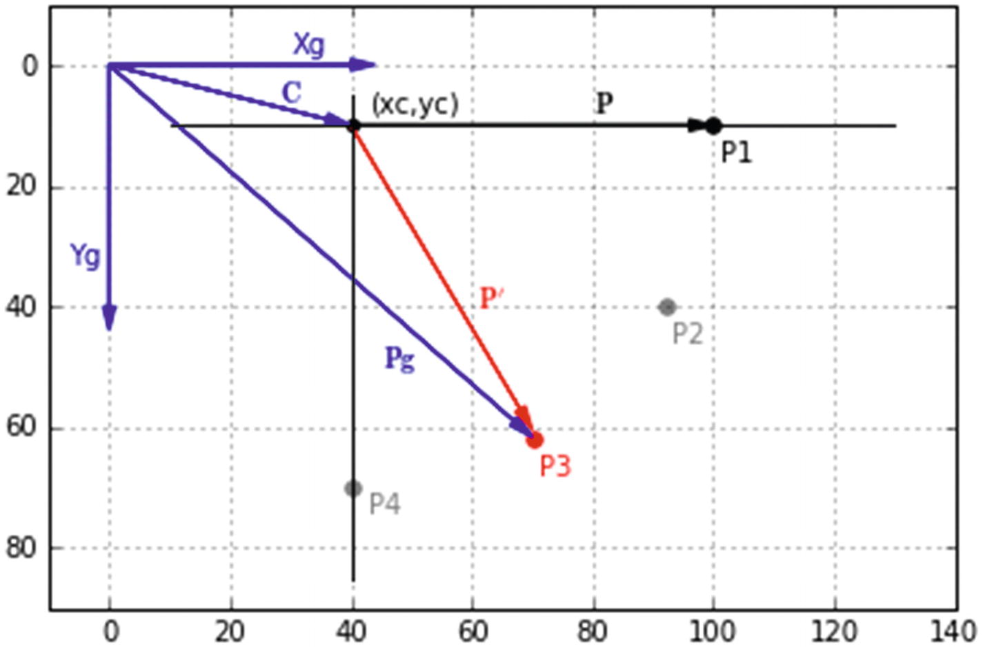
As an illustration of the above concepts, Listing 2-10 rotates a point P1 about (xc,yc) from its original unrotated location at (xp,yp)=(60,0) in 30 degree increments. Results are shown in Figure 2-15. The coordinates of the center of rotation, (xc,yc), are set in lines 16 and 17.

Lines 28-37 of Listing 2-10 define a function rotz(xp1,yp1,Rz), which uses the elements of the transformation matrix [Rz] in Equations 2-31 through 2-34 and the angle of rotation Rz to calculate and return the transformed (rotated and translated) coordinates (xg,yg). Lines 35 and 36 in function rotz relate the local coordinates to the xg,yg system for plotting. Note that rotz rotates each point and simultaneously translates it by xc and yc in lines 35 and 36. This puts the coordinates in the global system ready for plotting. You are rotating the point four times: Rz=0,30,60,90. The use of the function rotz(xp,yp,Rz) enables you to avoid coding the transformation for every point.

Lines 39 and 40 set the original coordinates of P to (60,0). It is important to note that these coordinates are relative to the center of rotation (xc,yc). Line 43 starts the calculation of the first point. This is at Rz=0. Line 44 converts Rz from degrees to radians. Later, I will show how to use the radians() function to do this. Line 45 invokes the function rotz(xp,yp,Rz). xp and yp were set in lines 39 and 40; Rz was set in line 43. The function returns the coordinates of the rotated point (xg,yg) in line 37. Since Rz was zero in this first transformation, they are the same as the coordinates of the unrotated point P1.

The plotting of point P2 begins in line 50. You set the angle of rotation to 30 degrees in line 50. The routine is the same as before and P2 is plotted as a grey point. Sections P3 and P4 increase Rz to 60 and 90 degrees, plotting the red and final grey point.

Lines 74, 77, 80, and 83 illustrate the use of Latex in printing text on a plot. Looking at line 74, for example,

plt.text(28,6,r'$mathbf{C}$',color='k')

the text starts at coordinates xg=28, yg=6. As discussed in Chapter 1, the r tells Python to treat the string as raw. This keeps the backward slashes needed by the Latex code between the dollar signs; in this case, $mathbf{C}$. mathbf{} makes whatever is between the braces {} bold. In line 80, ^{prime} places a superscript prime next to P. This won’t work if the prefix r is not included.

1
2   """
3   2DROT1
4   """
5   import matplotlib.pyplot as plt
6   import numpy as np
7
8   plt.axis([-10,140,90,-10])
9   plt.axis('on')
10  plt.grid(True)
11
12  #————————————————————————–axes
13  plt.arrow(0,0,40,0,head_length=4,head_width=2,color='b')
14  plt.arrow(0,0,0,40,head_length=4,head_width=2,color='b')
15
16  xc=40
17  yc=10
18
19  plt.plot([xc-30,xc+90],[yc,yc],linewidth=1,color='k') #—-X
20  plt.plot([xc,xc],[yc-5,yc+75],linewidth=1,color='k') #—-Y
21
22  plt.text(30,-2,'Xg',color='b')
23  plt.text(-7,33,'Yg',color='b')
24  plt.scatter(xc,yc,s=20,color='k')
25  plt.text(xc+3,yc-2,'(xc,yc)')
26
27  #—————————————————–define rotation matrix rz
28  def rotz(xp,yp,rz): #——–xp,yp=un-rotated coordinates relative to xc,yc
29       c11=np.cos(rz)
30       c12=-np.sin(rz)
31       c21=np.sin(rz)
32       c22=np.cos(rz)
33       xpp=xp*c11+yp*c12 #—-xpp,ypp=rotated coordinates relative to xc,yc
34       ypp=xp*c21+yp*c22
35       xg=xc+xpp #—-xg,yg=rotated coordinates relative to xg,yg
36       yg=yc+ypp
37       return [xg,yg]
38
39  xp=60 #————————————-coordinates of first point P1 relative to xc,yc
40  yp=0
41
42  #——————————————————————————————P1
43  rz=0
44  rz=rz*np.pi/180
45  [xg,yg]=rotz(xp,yp,rz)
46  plt.scatter(xg,yg,s=30,color='k' )
47  plt.text(xg+1,yg+6,'P1',color='k')
48
49  #——————————————————————————————————P2
50  rz=30
51  rz=rz*np.pi/180
52  [xg,yg]=rotz(xp,yp,rz)
53  plt.scatter(xg,yg,s=30,color='grey')
54  plt.text(xg+1,yg+6,'P2',color='grey')
55
56  #——————————————————————————————————P3
57  rz=60
58  rz=rz*np.pi/180
59  [xg,yg]=rotz(xp,yp,rz)
60  plt.scatter(xg,yg,s=30,color='r')
61  plt.text(xg+1,yg+6,'P3',color='r')
62  xpp3=xg #——save for later in line 76
63  ypp3=yg
64
65  #——————————————————————————————————P4
66  rz=90
67  rz=rz*np.pi/180
68  [xg,yg]=rotz(xp1,yp1,rz)
69  plt.scatter(xg,yg,s=30,color='grey')
70  plt.text(xp2+1,yp2+6,'P4',color='grey')
71
72  #————————————————————————————————————————————————plot vectors
73  plt.arrow(0,0,xc-4,yc-1,head_length=4,head_width=2,color='k')
74  plt.text(28,6,r'$mathbf{C}$',color='k')
75
76  plt.arrow(0,0,xpp3-3,ypp3-3,head_length=4,head_width=2,color='b')
77  plt.text(45,50,r'$mathbf{Pg}$',color='b')
78
79  plt.arrow(xc,yc,xpp3-2-xc,ypp3-5-yc,head_length=4,head_width=2,color='r')
80  plt.text(61,40,r'$mathbf{P^{prime}}$',color='r')
81
82  plt.arrow(xc,yc,xp-4,yp,head_length=4,head_width=2,color='k')
83  plt.text(80,yc-2,r'$mathbf{P}$',color='k')
84
85  plt.show()
Listing 2-10

Program 2DROT1

../images/456962_1_En_2_Chapter/456962_1_En_2_Fig16_HTML.jpg
Figure 2-16

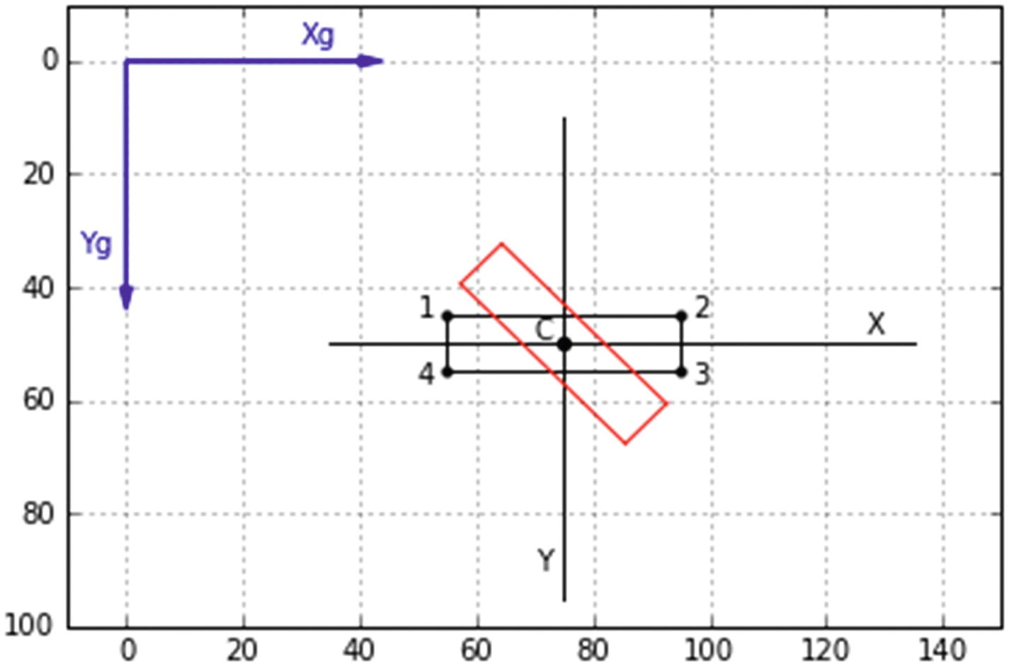
Rotation of a rectangle around its center from Listing 2-11

Next, you rotate a rectangle around its center, as shown in Figure 2-16. The center of rotation is point c at (xc,yc). The black rectangle shows the rectangle in its unrotated orientation. Its corners are numbered 1-4, as shown. The program plots the unrotated rectangle and then rotates it around point c to the rotated position and displays it in red.

Since the rectangle is defined by its corner points, you can rotate it by rotating the corners around c. The methodology is detailed in Listing 2-11. First, you plot the unrotated rectangle (black). The local coordinates of its four corner points are specified relative to the center of rotation c in lines 42-49. The points are labelled and plotted as dots in lines 51-58 where the local coordinates are converted to global by adding xc and yc in lines 55-58.

Next, you connect the corners by lines. Lines 61-68 translate the local corner coordinates by xc and yc. These points are labelled xg and yg to indicate that they are relative to the global plotting axes. They are set up as lists in lines 70 and 71, and then plotted in line 73, which draws lines between sequential xg,yg pairs.

Note the sequence of coordinate pairs in lines 70 and 71. When line 73 is invoked, it connects (xg1,yg1) to (xg2,yg2), then (xg2,yg2) to (xg3,yg3), and so on. But when it gets to corner 4, it has to connect corner 4 back to corner 1 in order to close the rectangle; hence you have (xg4,yg4) connected to (xg1,yg1) at the end of 70 and 71.

The plotting of the rotated rectangle begins at line 76. Rz is the angle of rotation. It is set to 45 degrees here and then converted from degrees to radians in line 77 (you could have used the radians() function to do this).

The function rotz(xp,yp,Rz) is defined in lines 29-38. The elements of the rotation transformation matrix shown in Equations 2-31 through 2-34 are evaluated in lines 30-33. xp and yp are the coordinates of an unrotated point. xpp and ypp (xp′ and yp′), coordinates in the rotated system, are evaluated in lines 34 and 35 using Equations 2-24 and 2-25. xg and yg, the coordinates in the global system after rotation and translation, are evaluated in lines 36-37 in accordance with Equations 2-35 and 2-36. Note that these lines rotate the points and simultaneously translate them relative to point c. The transformed coordinates are returned as a list in line 38.

Lines 80-101 transform each of the corner coordinates one by one by invoking function rotz(xp,yp,Rz). For example, lines 80-83 transform corner 1 from local, unrotated coordinates xp1,yp1 to global coordinates xg and yg. The remaining three points are transformed in the same way. The lines connecting the corners are plotted in red in lines 104-107 using lists.

1   """
2   2DROTRECTANGLE
3   """
4
5   import matplotlib.pyplot as plt
6   import numpy as np
7
8   plt.axis([-10,150,100,-10])
9   plt.axis('on')
10  plt.grid(True)
11
12  #————————————————————————————————————————————————————–axes
13  plt.arrow(0,0,40,0,head_length=4,head_width=2,color='b')
14  plt.arrow(0,0,0,40,head_length=4,head_width=2,color='b')
15  plt.text(30,-3,'Xg',color='b')
16  plt.text(-8,34,'Yg',color='b')
17
18  xc=75 #————————————————–center of rotation
19  yc=50
20  plt.plot([xc-40,xc+60],[yc,yc],linewidth=1,color='grey') #—-X
21  plt.plot([xc,xc],[yc-40,yc+45],linewidth=1,color='grey') #—-Y
22  plt.text(127,48,'X')
23  plt.text(70,90,'Y')
24
25  plt.scatter(xc,yc,s=20,color='k') #—plot center of rotation
26  plt.text(70,49,'c')
27
28  #———————————————————————————————————————————-define function rotz
29  def rotz(xp,yp,rz):
30      c11=np.cos(rz)
31      c12=-np.sin(rz)
32      c21=np.sin(rz)
33      c22=np.cos(rz)
34      xpp=xp*c11+yp*c12 #————-relative to xc,yc
35      ypp=xp*c21+yp*c22
36      xg=xc+xpp #—-relative to xg,yg
37      yg=yc+ypp
38      return [xg,yg]
39
40  #——————————————————————————————————————————–plot unrotated rectangle
41  #—————————————————–rectangle corner coordinates in X,Y system
42  xp1=-20
43  xp2=+20
44  xp3=+20
45  xp4=-20
46  yp1=-5
47  yp2=-5
48  yp3=+5
49  yp4=+5
50
51  plt.text(50,45,'1') #——————-label
52  plt.text(97,45,'2')
53  plt.text(97,57,'3')
54  plt.text(50,57,'4')
55  plt.scatter(xp1+xc,yp1+yc,s=10,color='k')
56  plt.scatter(xp2+xc,yp2+yc,s=10,color='k')
57  plt.scatter(xp3+xc,yp3+yc,s=10,color='k')
58  plt.scatter(xp4+xc,yp4+yc,s=10,color='k')
59
60  #——————————————————————————–plot unrotated rectangle
61  xg1=xc+xp1 #——————–corner coordinates in Xg,Yg system
62  yg1=yc+yp1
63  xg2=xc+xp2
64  yg2=yc+yp2
65  xg3=xc+xp3
66  yg3=yc+yp3
67  xg4=xc+xp4
68  yg4=yc+yp4
69
70  xg=[xg1,xg2,xg3,xg4,xg1]
71  yg=[yg1,yg2,yg3,yg4,yg1]
72
73  plt.plot((xg),(yg),color='k')
74
75  #———————————————————————–rotate rectangle corner coordinates
76  rz=45
77  rz=rz*np.pi/180
78
79  #———————————————————————————————————–point 1
80  xp=xp1
81  yp=yp1
82  [xg,yg]=rotz(xp,yp,rz)
83  [xg1,yg1]=[xg,yg]
84
85  #———————————————————————————————————–point 2
86  xp=xp2
87  yp=yp2
88  [xg,yg]=rotz(xp,yp,rz)
89  [xg2,yg2]=[xg,yg]
90
91  #———————————————————————————————————–point 3
92  xp=xp3
93  yp=yp3
94  [xg,yg]=rotz(xp,yp,rz)
95  [xg3,yg3]=[xg,yg]
96
97  #———————————————————————————————————–point 4
98  xp=xp4
99  yp=yp4
100 [xg,yg]=rotz(xp,yp,rz)
101 [xg4,yg4]=[xg,yg]
102
103 #———————————————————————————————————–plot rotated rectangle
104 xg=[xg1,xg2,xg3,xg4,xg1]
105 yg=[yg1,yg2,yg3,yg4,yg1]
106
107 plt.plot(xg,yg,color='r')
108
109 plt.show()
Listing 2-11

Program 2DROTRECTANGLE

To summarize the procedure, you first construct the object, in this case a simple rectangle, using points located at coordinates xp,yp in the local x,y system. This is done by specifying the coordinates relative to the center of rotation at c. Next, you specify Rz, evaluate the elements of the transformation matrix, transform each coordinate by Rz, translate the rotated points by xc,yc to get everything into the global xg,yg system, and then plot. The transformations are carried out by the function rotz(xp,yp,rz), which simultaneously rotates and translates the coordinates into the xg,yg system for plotting. In this case, you transformed all the coordinates first and then plotted at the end using lists. In some programs, you will plot points or lines immediately after transforming.

Next, you rotate a rectangle about its lower left corner. This is shown in Figure 2-17. The program that does this (not listed) is similar to Listing 2-11 except the center of rotation is changed to
$$ xc=55 $$
(2-40)
$$ yc=55 $$
(2-41)
and the corner coordinates are changed to
$$ xp1=0 $$
(2-42)
$$ xp2=+50 $$
(2-43)
$$ xp3=+50 $$
(2-44)
$$ xp4=0 $$
(2-45)
$$ yp1=-10 $$
(2-46)
$$ yp2=-10 $$
(2-47)
$$ yp3=+0 $$
(2-48)
$$ yp4=+0 $$
(2-49)
These dimensions are relative to the center of rotation, (xc,yc).
../images/456962_1_En_2_Chapter/456962_1_En_2_Fig17_HTML.jpg
Figure 2-17

Rotation of a rectangle about a corner

The center of rotation c does not have to be contiguous with the object; you could put it anywhere as long as the corner coordinates relative to the center of rotation are updated.

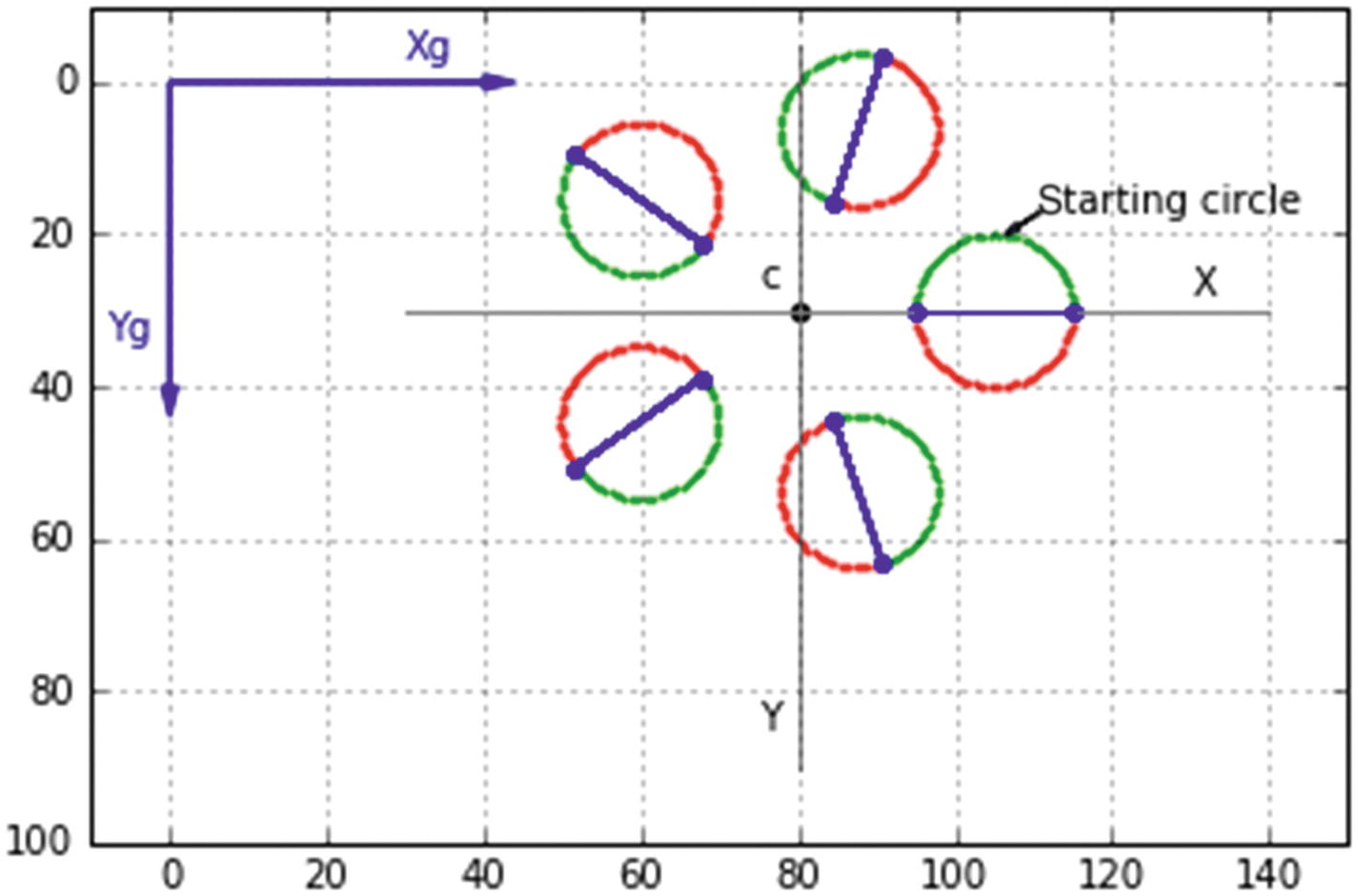
Figure 2-18 shows an example of constructing and rotating a circular object. Obviously, without some distinctive feature, you wouldn’t be able to see if a circle had been rotated so you make the top half of the starting circle green and the bottom half red. You also add a bar across the diameter with dots at each end. Figure 2-19 shows the model used by Listing 2-12 to generate Figure 2-18.

As shown in Figures 2-19 and 2-18, and referring to Listing 2-12, you construct the starting circle with a center at xcc,ycc in program lines 41 and 42. It has a radius r=10, which is set in line 43. The angle p starts at p1=0 and goes to p2=2π in steps dp in lines 45-47. Note that you are not using the angle definition Rz since p is a local angle about point xcc,ycc (the center of the circle), not xc,yc, the center of rotation. Points along the circle’s perimeter are calculated in lines 55 and 56 in local coordinates. When alpha=0, this produces the starting circle.

The use of alpha in the function call in line 57 illustrates that you can use any name for the angle, even though Rz was used in the function definition in line 29. You are passing a number from a function call to a function. It doesn’t matter what name it has on either end; the value received by the function will be the same as in the call to that function.
../images/456962_1_En_2_Chapter/456962_1_En_2_Fig18_HTML.jpg
Figure 2-18

Circles rotated about point c from Listing 2-12

../images/456962_1_En_2_Chapter/456962_1_En_2_Fig19_HTML.jpg
Figure 2-19

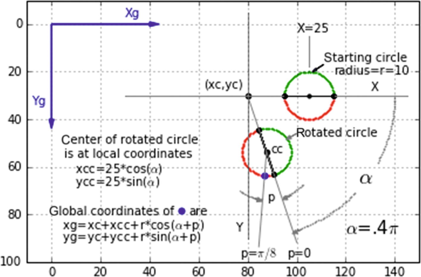
Model used by Listing 2-12

When alpha >0, the other four circles are drawn. The alpha loop starting at line 53 moves the circle’s center (xcc,ycc) clockwise around the center of rotation in steps dalpha, which is set in line 51. The local coordinates are transformed in line 57 by invoking rotz. Alpha’s inclusion in the rotz function call has the effect of rotating the circle about its own center (xcc,ycc). Lines 58-61 determine if each circumferential point lies between p=0 and p=π. If so, the point is plotted as red, otherwise as green. Thus, the circle’s top half is red, its bottom half is green. Lines 62-70 plot the diametrical bars and points.

An important feature of this approach is that not only is the circle’s center rotated around point c in steps dalpha, but each circle itself is rotated about its own center, as can be seen from the reorientation of the red and green sectors and the diametrical bars in the rotated circles. In the next program, you will rotate each circle’s center around point c while keeping each circle unrotated about its own center.

Why am I using circles in this demonstration ? Primarily because it illustrates how to construct circular shapes at any location relative to a center of rotation and rotate them. It illustrates the importance of being aware of the location of the center of rotation; it isn’t necessarily the same as the center of the circle.

In this case, you are rotating in the plane of the circle, which admittedly isn’t very illuminating. But later, these concepts will become useful when I show how to rotate objects, such as a circle, in three dimensions. In the case of a circle, when rotated out of its plane, it produces an oval, which is essential in portraying circular and spherical objects such as cylinders and spheres in three dimensions. Simply rotate a circle out of plane about a coordinate direction and you get an oval.

1   """
2   2DROTCIRCLE1
3   """
4
5   import matplotlib.pyplot as plt
6   import numpy as np
7
8   plt.axis([-10,150,100,-10])
9   plt.axis('on')
10  plt.grid(True)
11
12  #————————————————————————————————————————————————————–axes
13  plt.arrow(0,0,40,0,head_length=4,head_width=2,color='b')
14  plt.arrow(0,0,0,40,head_length=4,head_width=2,color='b')
15  plt.text(30,-3,'Xg',color='b')
16  plt.text(-8,34,'Yg',color='b')
17
18  xc=80 #————————————————–center of rotation
19  yc=30
20  plt.plot([xc-50,xc+60],[yc,yc],linewidth=1,color='grey') #—-X
21  plt.plot([xc,xc],[yc-35,yc+60],linewidth=1,color='grey') #—-Y
22  plt.text(xc+50,yc-2,'X')
23  plt.text(xc-5,yc+55,'Y')
24
25  plt.scatter(xc,yc,s=20,color='k') #—plot center of rotation
26  plt.text(xc-5,yc-3,'c')
27
28  #———————————————————————————————————————–define rotation matrix Rz
29  def rotz(xp,yp,rz):
30       c11=np.cos(rz)
31       c12=-np.sin(rz)
32       c21=np.sin(rz)
33       c22=np.cos(rz)
34       xpp=xp*c11+yp*c12 #—-rotated coordinates relative to xc,yc
35       ypp=xp*c21+yp*c22
36       xg=xc+xpp #—-rotated coordinates relative to xg,yg
37       yg=yc+ypp
38       return [xg,yg]
39
40  #——————————————————————————————————————————————————plot circles
41  xcc=25 #–xcc,ycc=center of starting circle in local X,Y system
42  ycc=0
43  r=10 #—radius
44
45  p1=0 #——–p1,p2=angles around circle center
46  p2=2*np.pi
47  dp=(p2-p1)/100
48
49  alpha1=0 #—–angles around xc,yc
50  alpha2=2*np.pi
51  dalpha=(alpha2-alpha1)/5
52
53  for alpha in np.arange(alpha1,alpha2,dalpha):
54        for p in np.arange(p1,p2,dp):
55             xp=xcc+r*np.cos(p) #——xp,yp=coordinates relative to local X,Y system
56             yp=ycc+r*np.sin(p)
57             [xg,yg]=rotz(xp,yp,alpha)
58             if p < np.pi:
59                  plt.scatter(xg,yg,s=1,color='r') #——plot lower half red
60             else:
61                  plt.scatter(xg,yg,s=1,color='g') #——plot upper half green
62             xp1=xcc+r #——plot diameter bars and bar end points
63             yp1=0
64             [xg1,yg1]=rotz(xp1,yp1,alpha)
65             xp2=xcc-r
66             yp2=0
67             [xg2,yg2]=rotz(xp2,yp2,alpha)
68             plt.plot([xg1,xg2],[yg1,yg2],color='b')
69             plt.scatter(xg1,yg1,s=10,color='b')
70             plt.scatter(xg2,yg2,s=10,color='b')
71
72  plt.text(xc+31,yc-13,'starting circle')
73  plt.arrow(xc+31,yc-13,-3,2,head_length=2,head_width=1)
74
75  plt.show()
Listing 2-12

Program 2DROTCIRCLE1

As shown in Figure 2-20, Listing 2-13 rotates the starting circle through increments of angle dalpha while keeping the orientation of each circle unchanged. The program is similar to the preceding one, with the exception that only the local center of each circle is rotated about point c while the circumferential points, as defined by the starting circle, remain unrotated. The program should be self-explanatory.

Note the difference between Listings 2-12 and 2-13. In Listing 2-12, the rotation takes place in lines 53-70. At each angle alpha, the coordinates of each point around the circle’s circumference are determined in lines 55 and 56. These are then transformed in line 57 using the function rotz(xp,yp,alpha). That is, each point around the circumference is rotated by the angle alpha. This has the effect of rotating the entire circle, as shown in Figure 2-18. In Listing 2-13, however, the plotting is done in lines 41-68. Here only the circle’s center is rotated in lines 50 and 51. In line 55, rotz(xp,yp,0) uses the angle p=0 in its argument. This has the effect of not rotating the circle itself, only its center, as shown in Figure 2-20.
../images/456962_1_En_2_Chapter/456962_1_En_2_Fig20_HTML.jpg
Figure 2-20

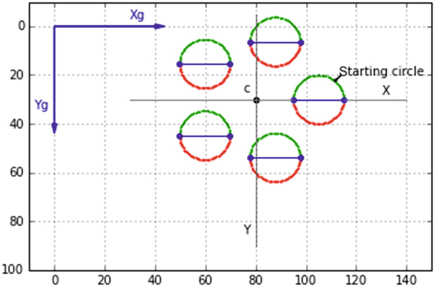
Circles with centers rotated about point c from Listing 2-13

Which method of rotation should you use: that shown in Figure 2-18 or 2-20? It depends on your application. In one you may want the entire object, including the points that comprise it, to rotate about a center whereas in another you may want only the center of the object to rotate while the object retains its original orientation. See Figure 2-21.
../images/456962_1_En_2_Chapter/456962_1_En_2_Fig21_HTML.jpg
Figure 2-21

Model used by Listing 2-13

1   """
2   2DROTCIRCLE2
3   """
4
5   import matplotlib.pyplot as plt
6   import numpy as np
7
8   plt.axis([-10,150,100,-10])
9   plt.axis('on')
10  plt.grid(True)
11
12  #————————————————————————————————————————————————————–axes
13  plt.arrow(0,0,40,0,head_length=4,head_width=2,color='b')
14  plt.arrow(0,0,0,40,head_length=4,head_width=2,color='b')
15  plt.text(30,-3,'Xg',color='b')
16  plt.text(-8,34,'Yg',color='b')
17
18  xc=80 #—————————————————center of rotation
19  yc=30
20  plt.plot([xc-50,xc+60],[yc,yc],linewidth=1,color='grey') #—-X
21  plt.plot([xc,xc],[yc-35,yc+60],linewidth=1,color='grey') #—-Y
22  plt.text(xc+50,yc-2,'X')
23  plt.text(xc-5,yc+55,'Y')
24
25  plt.scatter(xc,yc,s=20,color='k') #—plot center of rotation
26  plt.text(xc-5,yc-3,'c')
27
28  #————————————————————————————————————————define rotation matrix Rz
29  def rotz(xp,yp,rz):
30       c11=np.cos(rz)
31       c12=-np.sin(rz)
32       c21=np.sin(rz)
33       c22=np.cos(rz)
34       xpp=xp*c11+yp*c12 #—-relative to xc,yc
35       ypp=xp*c21+yp*c22
36       xg=xc+xpp #—-relative to xg,yg
37       yg=yc+ypp
38       return [xg,yg]
39
40  #————————————————————————————————————————————plot circles
41  p1=0
42  p2=2*np.pi
43  dp=(p2-p1)/100
44
45  alpha1=0
46  alpha2=2*np.pi
47  dalpha=(alpha2-alpha1)/5
48
49  for alpha in np.arange(alpha1,alpha2,dalpha):
50        xcc=25*np.cos(alpha)
51        ycc=25*np.sin(alpha)
52        for p in np.arange(p1,p2,dp):
53             xp=xcc+r*np.cos(p)
54             yp=ycc+r*np.sin(p)
55             [xg,yg]=rotz(xp,yp,0)
56             if p < np.pi:
57                  plt.scatter(xg,yg,s=1,color='r')
58             else:
59                  plt.scatter(xg,yg,s=1,color='g')
60             xp1=xcc+r
61             yp1=ycc+0
62             [xg1,yg1]=rotz(xp1,yp1,0)
63             xp2=xcc-r
64             yp2=ycc+0
65             [xg2,yg2]=rotz(xp2,yp2,0)
66             plt.plot([xg1,xg2],[yg1,yg2],color='b')
67             plt.scatter(xg1,yg1,s=10,color='b')
68             plt.scatter(xg2,yg2,s=10,color='b')
69
70  plt.text(xc+34,yc-10,'starting circle')
71  plt.arrow(xc+34,yc-10,-2,2,head_length=1,head_ width=1)
72
73  plt.show()
Listing 2-13

Program 2DROTCIRCLE2

2.10  Summary

In this chapter, you saw how to use dots and lines to construct shapes in two dimensions. You learned the concept of relative coordinates, specifically the local system , which is used to construct an image with coordinate values relative to a center, which in the case of rotation may be used as the center of rotation, and the global system which is used for plotting. You saw how local coordinates must be transformed into the global system for plotting, the origin of the global system being defined through the plt.axes() function. You saw how to construct lines from dots; arrange colored dots in artistic patterns; and draw arcs, discs, circles, and ellipses using dots and line segments. Then you learned about the concepts of translation (easy) and rotation (not so easy). You applied all this to points, rectangles, and circles. In the next chapter, you will extend these ideas to three dimensions.

..................Content has been hidden....................

You can't read the all page of ebook, please click here login for view all page.
Reset
3.15.143.181